Quantum Coding with Entanglement

Quantum error correction theory [16, 21, 22, 17, 19] now plays a prominent role in the practical realization and engineering of quantum computing and communication devices. The first quantum error-correcting codes [16, 21, 22, 19] are strikingly similar to classical block codes [23] in their operation and performance. Quantum error-correcting codes restore a noisy, decohered quantum state to a pure quantum state. Any future quantum information processing device will operate faithfully only if it employs an error correction scheme. This scheme can be an active scheme [17], a passive scheme [24, 25, 26], or a combination of both techniques [27, 28, 29, 30, 31].

The field of quantum error correction has rapidly expanded in recent years because there are so many ways in which one can correct quantum error. We briefly introduce three notable developments in the theory—these three are by no means exhaustive. The developments include the stabilizer formalism, the entanglement-assisted stabilizer formalism, and the convolutional stabilizer formalism.

Quantum error correction theory gives practical ways to build codes for protection of quantum information against decoherence. A quantum code typically encodes some number $k$ of information qubits into a larger number $n$ of physical qubits. We say that the rate of quantum communication for this code is $k/n$.

One may ask the question: what is the maximum rate of quantum communication for a given noisy quantum communication channel? This question is the fundamental question of quantum Shannon theory and the answer to it is a quantity known as the capacity of the quantum channel for quantum communication, or more simply, the quantum capacity [37, 38, 39, 61]. Quantum Shannon theory has many other questions. What is the rate of classical communication for a noisy quantum communication channel? What is the rate if the sender and receiver have access to entanglement? What is the rate of simultaneous classical and quantum communication? The list of questions goes on and on.

The goal of quantum Shannon theory is to quantify the amount of quantum communication, classical communication, and entanglement required for various information processing tasks [37, 38, 39, 61]. Quantum teleportation and superdense coding provided the initial impetus for quantum Shannon theory because these protocols demonstrate that we can combine entanglement, noiseless quantum communication, and noiseless classical communication to transmit quantum or classical information. In practice, the above resources are not noiseless because quantum systems decohere by interacting with their surrounding environment. Quantum Shannon theory is a collection of capacity theorems that determine the ultimate limits for noisy quantum communication channels. Essentially all quantum protocols have been unified as special cases of a handful of abstract protocols [61].

The techniques in quantum Shannon theory determine the asymptotic limits for communication, but these techniques do not produce practical ways of realizing these limits. This same practical problem exists with classical Shannon theory because random coding techniques determine the limit of a noisy classical communication channel [62].

This thesis represents a significant contribution to quantum error correction theory. In it, we give several methods for designing quantum codes. These methods should be useful in the future when coherent quantum encoding devices are available. The quantum code designer will have a plethora of techniques to exploit for protecting quantum information and the techniques in this thesis should be part of the arsenal.

A quick glance over the thesis reveals that much of the mathematics involves only linear algebra over matrices of binary numbers or binary polynomials. It is a testament to the strength of the theory that it reduces to this simple form. We show in detail especially in Chapters 2 and 4 how to reduce the theory to have this simple form. This thesis has contributions from the following publications [52, 67, 68, 69, 53, 51, 70].

We structure the thesis as follows. The next chapter introduces the stabilizer formalism for quantum error correction. We show in this chapter how to represent quantum codes with binary matrices. Chapter 3 introduces the entanglement-assisted stabilizer formalism and shows how to enhance the stabilizer formalism by assuming that the sender and receiver share entanglement. This chapter gives two contributions: a method for determining the encoding circuit for a quantum block code and a method to determine the minimal amount of entanglement that an entanglement-assisted code requires. Chapter 4 reviews the convolutional stabilizer formalism. In particular, it details the operation of a quantum convolutional code and shows how to simplify the mathematics with matrices whose entries are binary polynomials. Chapters 5, 6, and 7 form the heart of this thesis. They show how to construct entanglement-assisted quantum codes that have a convolutional structure. The techniques developed represent a significant extension of the entanglement-assisted stabilizer formalism. Chapter 8 presents a unifying structure for quantum error correction under which most current schemes for quantum error correction fall. We present a method for distilling entanglement in a convolutional manner in Chapter 9. The major benefit of all of the above convolutional methods is that we can import arbitrary high-performance classical codes to construct high-performance quantum codes.

The stabilizer formalism exploits elements of the Pauli group $\Pi$. The set $\Pi=\left\{I,X,Y,Z\right\}$ consists of the Pauli operators:

$$I\equiv\begin{bmatrix}1&0\\ 0&1\end{bmatrix},\ X\equiv\begin{bmatrix}0&1\\ 1&0\end{bmatrix},\ Y\equiv\begin{bmatrix}0&-i\\ i&0\end{bmatrix},\ Z\equiv\begin{bmatrix}1&0\\ 0&-1\end{bmatrix}.$$

The above operators act on a single qubit—a vector in a two-dimensional Hilbert space—and are the most important in formulating a quantum error-correcting code. Two crucial properties of these matrices are useful: each matrix in $\Pi$ has eigenvalues equal to $+1$ or $-1$, and any two matrices in $\Pi$ either commute or anticommute.

In general, a quantum error-correcting code uses $n$ physical qubits to protect a smaller set of information qubits against decoherence or quantum noise. An $n$-qubit quantum error-correcting code employs elements of the Pauli group $\Pi^{n}$. The set $\Pi^{n}$ consists of $n$-fold tensor products of Pauli operators:

$$\Pi^{n}=\left\{e^{i\phi}A_{1}\otimes\cdots\otimes A_{n}:\forall j\in\left\{1,\ldots,n\right\},\ \ A_{j}\in\Pi,\ \ \phi\in\left\{0,\pi/2,\pi,3\pi/2\right\}\right\}.$$

(2.1)

Matrices in $\Pi^{n}$ act on a $2^{n}$-dimensional complex vector, or equivalently, an $n$-qubit quantum register. We omit tensor product symbols in what follows so that $A_{1}\cdots A_{n}\equiv A_{1}\otimes\cdots\otimes A_{n}$. The above two crucial properties for the single-qubit Pauli group $\Pi$ still hold for the Pauli group $\Pi^{n}$ (up to an irrelevant phase for the eigenvalue property). The $n$-fold Pauli group $\Pi^{n}$ plays an important role in both the encoding circuit and the error-correction procedure of a quantum stabilizer code over $n$ qubits.

We can phrase the theory of quantum error correction in purely mathematical terms using elements of $\Pi^{n}$. Consider a matrix $g_{1}\in\Pi^{n}$ that is not equal to $\pm I$. Matrix $g_{1}$ then has two eigenspaces each of dimension $2^{n-1}$. We can identify one eigenspace with the eigenvalue $+1$ and the other eigenspace with eigenvalue $-1$. Consider a matrix $g_{2}\in\Pi^{n}$ different from both $g_{1}$ and the identity that commutes with $g_{1}$. Matrix $g_{2}$ also has two eigenspaces each of size $2^{n-1}$ and identified similarly by its eigenvalues $\pm 1$. Then $g_{1}$ and $g_{2}$ have simultaneous eigenspaces because they commute. These matrices together have four different eigenspaces, each of size $2^{n-2}$ and identified by the eigenvalues $\pm 1,\pm 1$ of $g_{1}$ and $g_{2}$ respectively. We can continue this process of adding more commuting and independent matrices to a set $\mathcal{S}$. The matrices in $\mathcal{S}$ are independent in the sense that no matrix in $\mathcal{S}$ is a product of two or more other matrices in $\mathcal{S}$. Adding more matrices from $\Pi^{n}$ to $\mathcal{S}$ continues to divide the eigenspaces of matrices in $\mathcal{S}$. In general, suppose $\mathcal{S}$ consists of $n-k$ independent and commuting matrices $g_{1}$, …, $g_{n-k}\in\Pi^{n}$. These $n-k$ matrices then have $2^{n-k}$ different eigenspaces each of size $2^{k}$ and identified by the eigenvalues $\pm 1$, …, $\pm 1$ of $g_{1}$, …, $g_{n-k}$ respectively. Consider that the Hilbert space of $k$ qubits has size $2^{k}$. A dimension count immediately suggests that we can encode $k$ qubits into one of the eigenspaces of $\mathcal{S}$. We typically encode these $k$ qubits into the simultaneous $+1$-eigenspace of $g_{1}$, …, $g_{n-k}$. This eigenspace is the codespace. The operators $g_{1},\ldots,g_{n-k}$ function in the same way as a parity check matrix does for a classical linear block code. An $\left[n,k\right]$ quantum error-correcting code encodes $k$ information qubits into the simultaneous $+1$-eigenspace of $n-k$ matrices $g_{1}$, …, $g_{n-k}\in\Pi^{n}$. Its stabilizer $\mathcal{S}$ is an abelian subgroup of the $n$-fold Pauli group $\Pi^{n}$: $\mathcal{S}\subset\Pi^{n}$. Note that it is possible to multiply the generators in the stabilizer together and obtain an equivalent representation of the stabilizer in much the same way that we can add vectors in a basis together and obtain an equivalent basis.

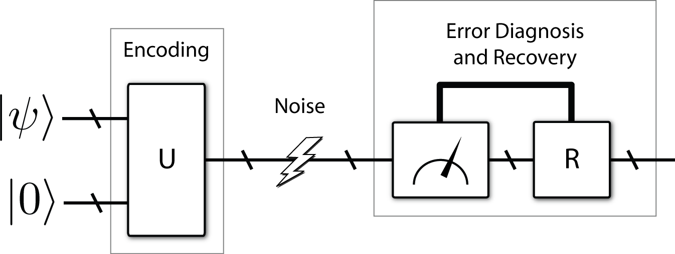
The operation of an $\left[n,k\right]$ quantum error-correcting code consists of four steps. Figure 2.1 highlights these steps.

1. (i).

   A unitary operation $U$ encodes both $k$ information qubits in a general state $\left|\psi\right\rangle$ and $n-k$ ancilla qubits in the state $\left|0\right\rangle^{\otimes n-k}$ into the simultaneous $+1$-eigenspace of the matrices $g_{1}$, …, $g_{n-k}$.

2. (ii).

   The sender transmits the $n$ encoded qubits by using the noisy quantum communication channel $n$ times.

3. (iii).

   The receiver performs quantum measurements of the $n-k$ matrices $g_{1}$, …, $g_{n-k}$ in the stabilizer $\mathcal{S}$. These measurements learn only about errors that may occur and do not disturb the encoded quantum information. Each measurement gives a bit result equal to $+1$ or $-1$, and the result of all the measurements is to project the $n$-qubit quantum register into one of the $2^{n-k}$ different eigenspaces of $g_{1}$, …, $g_{n-k}$. Suppose that no error occurs. Then the measurements project the $n$ qubits into the simultaneous $+1$-eigenspace and return a bit vector consisting of $n-k$ ones. This “projection of the error concept” is one of the fundamental notions in quantum error correction theory. It suffices to correct a discrete error set with support in the Pauli group $\Pi^{n}$ [16]. Now suppose that a quantum error in an error set $\mathcal{E}\subset\Pi^{n}$ occurs. The error takes the encoded quantum state out of the codespace and into one of the other $2^{n-k}-1$ orthogonal eigenspaces. The measurements can detect that an error has occurred because the result of the measurements is a bit vector differing from the all ones vector. The receiver can identify uniquely which error in $\mathcal{E}$ has occurred if the set $\mathcal{E}$ satisfies the following quantum error correction conditions:

   $$\forall E_{a},E_{b}\in\mathcal{E\ \ \ \ \ }\exists\ g_{i}\in\mathcal{S}:\left\{g_{i},E_{a}^{{\dagger}}E_{b}\right\}=0\text{ or }E_{a}^{{\dagger}}E_{b}\in\mathcal{S}.$$

   (2.2)

   The first condition corresponds to the active error-correcting capability of the code, and the second condition corresponds to its passive error-correcting capability.

4. (iv).

   If the receiver can identify which error occurs, he can then apply a unitary operation $R$ that is the inverse of the error. He finally performs a decoding unitary that decodes the $k$ information qubits.

We comment briefly on the encoding operation $U$. The encoding operation $U$ is a special type of unitary matrix called a Clifford operation. A Clifford operation $U$ is one that preserves elements of the Pauli group under conjugation: $A\in\Pi^{n}\Rightarrow UAU^{{\dagger}}\in\Pi^{n}$. The CNOT gate, the Hadamard gate $H$, and the phase gate $P$ suffice to implement any unitary matrix in the Clifford group [17]. A quantum code with the CSS structure needs only the CNOT and Hadamard gates for encoding and decoding. The matrix for the CNOT gate acting on two qubits is

$$\text{CNOT}=\begin{bmatrix}1&0&0&0\\ 0&1&0&0\\ 0&0&0&1\\ 0&0&1&0\end{bmatrix},$$

(2.3)

the matrix for the Hadamard gate $H$ acting on a single qubit is

$$H=\frac{1}{\sqrt{2}}\begin{bmatrix}1&1\\ 1&-1\end{bmatrix},$$

(2.4)

and the matrix for the phase gate $P$ acting on a single qubit is

$$P=\begin{bmatrix}1&0\\ 0&i\end{bmatrix}.$$

(2.5)

The standard basis for $\Pi^{1}$ is $X$ and $Z$ because any element of $\Pi^{1}$ is a product of elements in this generating set up to an irrelevant phase. The standard basis for elements of the two-qubit Pauli group $\Pi^{2}$ is as follows

$$\begin{array}[c]{cc}Z&I\end{array},\ \ \begin{array}[c]{cc}I&Z\end{array},\ \ \begin{array}[c]{cc}X&I\end{array},\ \ \begin{array}[c]{cc}I&X\end{array},$$

(2.6)

for the same reasons.

The Hadamard gate $H$ transforms the standard basis of $\Pi^{1}$ under conjugation as follows:

$$Z\rightarrow X,\ \ \ \ X\rightarrow Z$$

(2.7)

and the phase gate $P$ transforms the standard basis as follows:

$$Z\rightarrow Z,\ \ \ \ X\rightarrow Y.$$

(2.8)

For the CNOT gate, the first qubit is the “control” qubit and the second qubit is the “target” qubit. The CNOT gate transforms the standard basis of $\Pi^{2}$ under conjugation as follows

$$\begin{array}[c]{cc}Z&I\end{array}\rightarrow\begin{array}[c]{cc}Z&I\end{array},\ \ \ \begin{array}[c]{cc}I&Z\end{array}\rightarrow\begin{array}[c]{cc}Z&Z\end{array},\ \ \ \begin{array}[c]{cc}X&I\end{array}\rightarrow\begin{array}[c]{cc}X&X\end{array},\ \ \ \begin{array}[c]{cc}I&X\end{array}\rightarrow\begin{array}[c]{cc}I&X\end{array},$$

(2.9)

where the first qubit is the control and the second qubit is the target.

Section 3.5 of Chapter 3 details an algorithm that determines a Clifford encoding circuit for any stabilizer code or any entanglement-assisted stabilizer code (we review entanglement-assisted codes in the next chapter).

Another aspect of the theory of quantum error correction is later useful for our purposes in quantum convolutional coding. This aspect concerns the information qubits and the operators that change them. Consider that the initial unencoded state of a quantum error-correcting code is a simultaneous +1-eigenstate of the matrices $Z_{k+1},\ldots,Z_{n}$ where $Z_{i}$ has a $Z$ matrix operating on qubit $i$ and the identity $I$ on all other qubits. Therefore, the matrices $Z_{k+1},\ldots,Z_{n}$ constitute a stabilizer for the unencoded state. The initial unencoded logical operators for the $k$ information qubits are $Z_{1},X_{1},\ldots,Z_{k},X_{k}$. The encoding operation $U$ rotates the unencoded stabilizer matrices $Z_{k+1},\ldots,Z_{n}$ and the unencoded logical operators $Z_{1},X_{1},\ldots,Z_{k},X_{k}$ to the encoded stabilizer operators $\bar{Z}_{k+1}$, …, $\bar{Z}_{n}$ and the encoded logical operators $\bar{Z}_{1},\bar{X}_{1},\ldots,\bar{Z}_{k},\bar{X}_{k}$ respectively. The encoded matrices $\bar{Z}_{k+1},\ldots,\bar{Z}_{n}$ are respectively equivalent to the matrices $g_{1}$, …, $g_{n-k}$ in the discussion of the previous section.

The encoded operators obey the same commutation relations as their unencoded counterparts. We would violate the uncertainty principle if this invariance did not hold. Therefore, each of the encoded logical operators commutes with elements of the stabilizer $\mathcal{S}$. Let $A$ denote an arbitrary logical operator from the above set and let $\bar{Z}_{i}$ denote an arbitrary element of the stabilizer $\mathcal{S}$. The operator $A\bar{Z}_{i}$ (or equivalently $\bar{Z}_{i}A$) is an equivalent logical operator because $A\bar{Z}_{i}$ and $A$ have the same effect on an encoded state $\left|\bar{\psi}\right\rangle$:

$$\bar{Z}_{i}A\left|\bar{\psi}\right\rangle=A\bar{Z}_{i}\left|\bar{\psi}\right\rangle=A\left|\bar{\psi}\right\rangle.$$

(2.10)

We make extensive use of the above fact in our work.

The logical operators also provide a useful way to characterize the information qubits. Gottesman showed that the logical operators for the information qubits provide a straightforward way to characterize the information qubits as they progress through a quantum circuit [17]. As an example of this technique, he develops quantum teleportation in the stabilizer formalism. The logical operators at the beginning of the protocol are $X_{1}$ and $Z_{1}$ and become $X_{3}$ and $Z_{3}$ at the end of the protocol. This transformation implies that the quantum information in qubit one teleports to qubit three because the logical operators act on only qubit three at the end of the protocol. We use the same idea throughout this thesis to determine if our decoding circuits have truly decoded the information qubits.

A simple but useful mapping exists between elements of $\Pi$ and the binary vector space $\left(\mathbb{Z}_{2}\right)^{2}$. This mapping gives a simplification of quantum error correction theory. It represents quantum codes with binary vectors and binary operations rather than with Pauli operators and matrix operations respectively. We first give the mapping for the one-qubit case. Suppose $\left[A\right]$ is a set of equivalence classes of an operator $A$ that have the same phase:

$$\left[A\right]=\left\{\beta A\ |\ \beta\in\mathbb{C},\ \left|\beta\right|=1\right\}.$$

(2.11)

Let $\left[\Pi\right]$ be the set of phase-free Pauli operators where $\left[\Pi\right]=\left\{\left[A\right]\ |\ A\in\Pi\right\}$. Define the map $N:\left(\mathbb{Z}_{2}\right)^{2}\rightarrow\Pi$ as

(ℤ2)200011110.\begin{tabular}[c]{l|llll}$\Pi$&$I$&$X$&$Y$&$Z$\\ \hline\cr$\left(\mathbb{Z}_{2}\right)^{2}$&$00$&$01$&$11$&$10$\end{tabular}\ \ \ \ .

		$\mathrm{\Pi }$	$I$	$X$	$Y$	$Z$		(2.12)

Suppose $u,v\in\left(\mathbb{Z}_{2}\right)^{2}$. Let us employ the shorthand $u=\left[z|x\right]$ and $v=\left[z^{\prime}|x^{\prime}\right]$ where $z$, $x$, $z^{\prime}$, $x^{\prime}\in\mathbb{Z}_{2}$. For example, suppose $u=\left[0|1\right]$. Then $N\left(u\right)=X$. The map $N$ induces an isomorphism $\left[N\right]:\left(\mathbb{Z}_{2}\right)^{2}\rightarrow\left[\Pi\right]$ because addition of vectors in $\left(\mathbb{Z}_{2}\right)^{2}$ is equivalent to multiplication of Paulis up to a global phase:

$$\left[N\left(u+v\right)\right]=\left[N\left(u\right)\right]\left[N\left(v\right)\right].$$

(2.13)

We name this isomorphism the P2B isomorphism (for Pauli-to-binary isomorphism).

Let $\odot$ denote the symplectic product between two elements $u,v\in\left(\mathbb{Z}_{2}\right)^{2}$:

$$u\odot v\equiv zx^{\prime}-xz^{\prime}.$$

(2.14)

The symplectic product $\odot$ gives the commutation relations of elements of $\Pi$:

$$N\left(u\right)N\left(v\right)=\left(-1\right)^{\left(u\odot v\right)}N\left(v\right)N\left(u\right).$$

The symplectic product and the P2B isomorphism $\left[N\right]$ thus give a useful way to phrase Pauli relations in terms of binary algebra.

The extension of the above definitions and the P2B isomorphism $\left[N\right]$ to multiple qubits is straightforward. Let $\mathbf{A}=A_{1}\otimes\cdots\otimes A_{n}$ denote an arbitrary element of $\Pi^{n}$. We can similarly define the phase-free $n$-qubit Pauli group $\left[\Pi^{n}\right]=\left\{\left[\mathbf{A}\right]\ |\ \mathbf{A}\in\Pi^{n}\right\}$ where

$$\left[\mathbf{A}\right]=\left\{\beta\mathbf{A}\ |\ \beta\in\mathbb{C},\ \left|\beta\right|=1\right\}.$$

(2.15)

The group operation $\ast$ for the above equivalence class is as follows:

$$\left[\mathbf{A}\right]\ast\left[\mathbf{B}\right]\equiv\left[A_{1}\right]\ast\left[B_{1}\right]\otimes\cdots\otimes\left[A_{n}\right]\ast\left[B_{n}\right]=\left[A_{1}B_{1}\right]\otimes\cdots\otimes\left[A_{n}B_{n}\right]=\left[\mathbf{AB}\right].$$

(2.16)

The equivalence class $\left[\Pi^{n}\right]$ forms a commutative group under operation $\ast$. Consider the $2n$-dimensional vector space

$$\left(\mathbb{Z}_{2}\right)^{2n}=\left\{\left(\mathbf{z,x}\right):\mathbf{z},\mathbf{x}\in\left(\mathbb{Z}_{2}\right)^{n}\right\}.$$

(2.17)

It forms the commutative group $(\left(\mathbb{Z}_{2}\right)^{2n},+)$ with operation $+$ defined as binary vector addition. We employ the notation $\mathbf{u}=\left[\mathbf{z}|\mathbf{x}\right]$ and $\mathbf{v}=\left[\mathbf{z}^{\prime}|\mathbf{x}^{\prime}\right]$ to represent any two vectors $\mathbf{u,v}\in\left(\mathbb{Z}_{2}\right)^{2n}$ respectively. Each vector $\mathbf{z}$ and $\mathbf{x}$ has elements $\left(z_{1},\ldots,z_{n}\right)$ and $\left(x_{1},\ldots,x_{n}\right)$ respectively with similar representations for $\mathbf{z}^{\prime}$ and $\mathbf{x}^{\prime}$. The symplectic product $\odot$ of $\mathbf{u}$ and $\mathbf{v}$ is

$$\mathbf{u}\odot\mathbf{v\equiv}\sum_{i=1}^{n}z_{i}x_{i}^{\prime}-x_{i}z_{i}^{\prime}=\sum_{i=1}^{n}u_{i}\odot v_{i},$$

(2.18)

where $u_{i}=\left[z_{i}|x_{i}\right]$ and $v_{i}=\left[z_{i}^{\prime}|x_{i}^{\prime}\right]$. Let us define a map $\mathbf{N}:\left(\mathbb{Z}_{2}\right)^{2n}\rightarrow\Pi^{n}$ as follows:

$$\mathbf{N}\left(\mathbf{u}\right)\equiv N\left(u_{1}\right)\otimes\cdots\otimes N\left(u_{n}\right).$$

(2.19)

Let

$$\mathbf{X}\left(\mathbf{x}\right)\equiv X^{x_{1}}\otimes\cdots\otimes X^{x_{n}},\ \ \ \ \ \ \mathbf{Z}\left(\mathbf{z}\right)\equiv Z^{z_{1}}\otimes\cdots\otimes Z^{z_{n}},$$

(2.20)

so that $\mathbf{N}\left(\mathbf{u}\right)$ and $\mathbf{Z}\left(\mathbf{z}\right)\mathbf{X}\left(\mathbf{x}\right)$ belong to the same equivalence class:

$$\left[\mathbf{N}\left(\mathbf{u}\right)\right]=\left[\mathbf{Z}\left(\mathbf{z}\right)\mathbf{X}\left(\mathbf{x}\right)\right].$$

(2.21)

The map $\left[\mathbf{N}\right]:\left(\mathbb{Z}_{2}\right)^{2n}\rightarrow\left[\Pi^{n}\right]$ is an isomorphism for the same reason given in (2.13):

$$\left[\mathbf{N}\left(\mathbf{u+v}\right)\right]=\left[\mathbf{N}\left(\mathbf{u}\right)\right]\left[\mathbf{N}\left(\mathbf{v}\right)\right],$$

(2.22)

where $\mathbf{u,v}\in\left(\mathbb{Z}_{2}\right)^{2n}$. The symplectic product captures the commutation relations of any operators $\mathbf{N}\left(\mathbf{u}\right)$ and $\mathbf{N}\left(\mathbf{v}\right)$:

$$\mathbf{N\left(\mathbf{u}\right)N}\left(\mathbf{v}\right)=\left(-1\right)^{\left(\mathbf{u}\odot\mathbf{v}\right)}\mathbf{N}\left(\mathbf{v}\right)\mathbf{N}\left(\mathbf{u}\right).$$

(2.23)

The above P2B isomorphism and symplectic algebra are useful in making the relation between classical linear error correction and quantum error correction more explicit.

An example of a stabilizer code is the five qubit $\left[5,1\right]$ stabilizer code [75, 66]. It encodes $k=1$ logical qubit into $n=5$ physical qubits and protects against an arbitrary single-qubit error. Its stabilizer consists of $n-k=4$ Pauli operators:

$$\begin{array}[c]{ccccccc}g_{1}&=&X&Z&Z&X&I\\ g_{2}&=&I&X&Z&Z&X\\ g_{3}&=&X&I&X&Z&Z\\ g_{4}&=&Z&X&I&X&Z\end{array}$$

(2.24)

The above operators commute. Therefore the codespace is the simultaneous +1-eigenspace of the above operators. Suppose a single-qubit error occurs on the encoded quantum register. A single-qubit error is in the set $\left\{X_{i},Y_{i},Z_{i}\right\}$ where $A_{i}$ denotes a Pauli error on qubit $i$. It is straightforward to verify that any arbitrary single-qubit error has a unique syndrome. The receiver corrects any single-qubit error by identifying the syndrome and applying a corrective operation.

The mathematics developed in this chapter form the basis for the work in later chapters. In particular, the binary representation of quantum codes is important. The role of the “twisted” symplectic product plays an important role for the entanglement-assisted codes of the next chapter because it helps in determining the commutation relations of an arbitrary (not necessarily commuting) set of Pauli generators.

The fundamental unit of bipartite entanglement is the ebit. We must first understand the commutativity properties of the ebit before developing the entanglement-assisted formalism. We express the state $\left|\Phi^{+}\right\rangle$ of an ebit shared between a sender Alice and a receiver Bob as follows:

$$\left|\Phi^{+}\right\rangle\equiv\frac{\left|00\right\rangle^{AB}+\left|11\right\rangle^{AB}}{\sqrt{2}}.$$

(3.1)

The two operators that stabilize this ebit state are $X^{A}X^{B}$ and $Z^{A}Z^{B}$. These two operators commute,

$$\left[X^{A}X^{B},Z^{A}Z^{B}\right]=0,$$

but the local operators (operating only on either party) anticommute,

$$\left\{X^{A},Z^{A}\right\}=\left\{X^{B},Z^{B}\right\}=0.$$

The above commutation relations hint at a way that we can resolve anticommutativity in a set of generators. Suppose that we have two generators that anticommute. We can use an ebit of entanglement to resolve the anticommutativity in the two generators. We explain this idea in more detail in what follows.

We review the general construction of an entanglement-assisted code. An $\left[n,k;c\right]$ entanglement-assisted code employs $c$ ebits and $a$ ancilla qubits to encode $k$ information qubits. Suppose that there is a nonabelian subgroup $\mathcal{S}\subset\Pi^{n}$ of size $2c+a$. Application of the fundamental theorem of symplectic geometry^** * We loosely refer to this theorem as the fundamental theorem of symplectic geometry because of its importance in symplectic geometry and in quantum coding theory. [77] (Lemma 1 in [34]) states that there exists a minimal set of independent generators $\left\{\bar{Z}_{1},\ldots,\bar{Z}_{a+c},\bar{X}_{a+1},\ldots,\bar{X}_{a+c}\right\}$ for $\mathcal{S}$ with the following commutation relations:

	$\displaystyle\forall i,j\ \ \ \ \left[\bar{Z}_{i},\bar{Z}_{j}\right]$	$\displaystyle=0,\ \ \ \ \forall i,j\ \ \ \ \left[\bar{X}_{i},\bar{X}_{j}\right]=0,$		(3.2)
	$\displaystyle\forall i\neq j\ \ \ \ \left[\bar{X}_{i},\bar{Z}_{j}\right]$	$\displaystyle=0,\ \ \ \ \forall i\ \ \ \ \left\{\bar{X}_{i},\bar{Z}_{i}\right\}=0.$

The decomposition of $\mathcal{S}$ into the above minimal generating set determines that the code requires $a$ ancilla qubits and $c$ ebits. The parameters $a$ and $c$ generally depend on the set of generators in $\mathcal{S}$.

There exists a symplectic Gram-Schmidt orthogonalization procedure that gives the decomposition [35, 34, 51, 78]. Specifically, the algorithm performs row operations (multiplication of the Pauli generators) that do not affect the code’s error-correcting properties and thus gives a set of generators that form an equivalent code. The decomposition also minimizes the number of ebits required for the code and we prove this optimality in Section 3.6.

We present a simple stabilizer version of the symplectic Gram-Schmidt algorithm. Suppose we have a set of $m$ generators $g_{1}$, …, $g_{m}$. Consider $g_{1}$. It either commutes with all other generators or it anticommutes with at least one other generator. Remove it from the set if it commutes with all other generators. Now suppose that it does not, i.e., it anticommutes with one other generator $g_{i}$. Relabel $g_{2}$ as $g_{i}$ and vice versa. Recall that we can multiply generators without changing the error-correcting properties of the set of generators. So we perform several multiplications to change the commutation relations to have the standard commutation relations in (3.2). We perform the following manipulations on the generators $g_{3}$, …, $g_{m}$:

$$g_{j}=g_{j}\cdot g_{1}^{f\left(g_{2},g_{j}\right)}\cdot g_{2}^{f\left(g_{1},g_{j}\right)}\ \ \ \ \ \ \forall\ i\in\left\{3,\ldots,m\right\}$$

where the function $f$ is equal to zero if its two arguments commute and it is equal to one if its two arguments anticommute. (This function is the symplectic product.) Remove the generators $g_{1}$ and $g_{2}$ from the set. Repeat the algorithm on the remaining generators. When the algorithm finishes, all the “removed’ generators constitute the generators for the code and have the standard commutation relations in (3.2).

We can partition the nonabelian group $\mathcal{S}$ into two subgroups: the isotropic subgroup $\mathcal{S}_{I}$ and the entanglement subgroup $\mathcal{S}_{E}$. The isotropic subgroup $\mathcal{S}_{I}$ is a commuting subgroup of $\mathcal{S}$ and thus corresponds to ancilla qubits: $\mathcal{S}_{I}=\left\{\bar{Z}_{1},\ldots,\bar{Z}_{a}\right\}$. The elements of the entanglement subgroup $\mathcal{S}_{E}$ come in anticommuting pairs and thus correspond to halves of ebits: $\mathcal{S}_{E}=\left\{\bar{Z}_{a+1},\ldots,\bar{Z}_{a+c},\bar{X}_{a+1},\ldots,\bar{X}_{a+c}\right\}$. The two subgroups $\mathcal{S}_{I}$ and $\mathcal{S}_{E}$ play a role in the error-correcting conditions for the entanglement-assisted stabilizer formalism. An entanglement-assisted code corrects errors in a set $\mathcal{E}\subset\Pi^{n}$ if

$$\forall E_{1},E_{2}\in\mathcal{E}\ \ \ \ \ \ \ \ E_{1}^{{\dagger}}E_{2}\in\mathcal{S}_{I}\text{ or }E_{1}^{{\dagger}}E_{2}\in\Pi^{n}-\mathcal{Z}\left(\left\langle\mathcal{S}_{I},\mathcal{S}_{E}\right\rangle\right).$$

The conditions correspond to error pairs $E_{1},E_{2}$ in an error set $\mathcal{E}$. The first condition corresponds to the passive error-correcting capability of the code, and the second condition corresponds to its active error-correcting capability.

Figure 3.1 illustrates the operation of an entanglement-assisted stabilizer code. The following four steps explain the operation of an $\left[n,k;c\right]$ entanglement-assisted quantum code:

1. (i).

   The sender and receiver share $c$ ebits before quantum communication begins and the sender has $a$ ancilla qubits. The unencoded state is a simultaneous +1-eigenstate of the following operators:

   $$\left\{Z_{a+1}|Z_{1},\ldots,Z_{a+c}|Z_{c},X_{a+1}|X_{1},\ldots,X_{a+c}|X_{c},Z_{1},\ldots,Z_{a}\right\}.$$

   (3.3)

   The operators to the right of the vertical bars indicate the receiver’s half of the shared ebits. The sender encodes her $k$ information qubits with the help of $a$ ancilla qubits and her half of the $c$ ebits. The encoding operation is $U$ in Figure 3.1. The encoding unitary transforms the unencoded operators to the following encoded operators:

   $$\left\{\bar{Z}_{a+1}|Z_{1},\ldots,\bar{Z}_{a+c}|Z_{c},\bar{X}_{a+1}|X_{1},\ldots,\bar{X}_{a+c}|X_{c},\bar{Z}_{1},\ldots,\bar{Z}_{a}\right\}.$$

   (3.4)

2. (ii).

   The sender sends her $n$ qubits over a noisy quantum communication channel. The noisy channel affects these $n$ qubits only and does not affect the receiver’s half of the $c$ ebits.

3. (iii).

   The receiver combines his half of the $c$ ebits with those he receives from the noisy quantum channel. He performs measurements on all $n+c$ qubits to diagnose an error that may occur on the $n$ qubits.

4. (iv).

   After estimating which error occurs, the receiver performs a recovery operation that reverses the estimated error.

Let us write the local operators $X^{A}$ and $Z^{A}$ on the sender Alice’s side as respective symplectic vectors $h_{1}$ and $h_{2}$:

$$h_{1}=\left[\left.\begin{array}[c]{c}0\end{array}\right|\begin{array}[c]{c}1\end{array}\right],\ \ \ \ \ \ \ \ h_{2}=\left[\left.\begin{array}[c]{c}1\end{array}\right|\begin{array}[c]{c}0\end{array}\right].$$

The “symplectic product matrix” $\Omega$ of these two symplectic vectors is as follows:

$$\Omega=\left[\begin{array}[c]{cc}0&1\\ 1&0\end{array}\right].$$

(3.5)

We call this matrix the symplectic product matrix because its entries enumerate the symplectic products:

$$\left[\Omega\right]_{ij}=h_{i}\odot h_{j}\text{ \ \ \ }\forall i,j\in\left\{1,2\right\}.$$

(3.6)

The symplectic product matrix in (3.5) is so special for the purposes of this thesis that we give it the name $J\equiv\Omega$. It means that two generators have commutation relations that are equivalent to half of an ebit.

A general set of generators for a quantum block code can have complicated commutation relations. For a given set of generators, the commutation relations for the generators resulting from the symplectic Gram-Schmidt orthogonalization procedure have a special form. Their symplectic product matrix $\Omega$ has the standard form:

$$\Omega={\displaystyle\bigoplus\limits_{i=1}^{c}}J\oplus{\displaystyle\bigoplus\limits_{j=1}^{a}}\left[0\right]$$

(3.7)

where the large and small $\oplus$ correspond to the direct sum operation and $\left[0\right]$ is the one-element null matrix. The standard form above implies that the commutation relations of the $2c+a$ generators are equivalent to those of $c$ halves of ebits and $a$ ancilla qubits—the commutation relations are equivalent to those in (3.2).

We can interpret the rate of an entanglement-assisted code in three different ways [34, 35, 51]. Suppose that an entanglement-assisted quantum code encodes $k$ information qubits into $n$ physical qubits with the help of $c$ ebits.

1. (i).

   The “entanglement-assisted” rate assumes that entanglement shared between sender and receiver is free. Bennett et al. make this assumption when deriving the entanglement-assisted capacity of a quantum channel for sending quantum information [40, 41]. The entanglement-assisted rate is $k/n$ for a code with the above parameters.

2. (ii).

   The “trade-off’ rate assumes that entanglement is not free and a rate pair determines performance. The first number in the pair is the number of noiseless qubits generated per channel use, and the second number in the pair is the number of ebits consumed per channel use. The rate pair is $\left(k/n,c/n\right)$ for a code with the above parameters. Quantum information theorists have computed asymptotic trade-off curves that bound the rate region in which achievable rate pairs lie [61]. Brun et al.’s construction for an entanglement-assisted quantum block code minimizes the number $c$ of ebits given a fixed number $k$ and $n$ of respective information qubits and physical qubits [35, 34].

3. (iii).

   The “catalytic rate” assumes that bits of entanglement are built up at the expense of transmitted qubits [35, 34]. A noiseless quantum channel or the encoded use of noisy quantum channel are two different ways to build up entanglement between a sender and receiver. The catalytic rate of an $\left[n,k;c\right]$ code is $\left(k-c\right)/n$.

Which interpretation is most reasonable depends on the context in which we use the code. In any case, the parameters $n$, $k$, and $c$ ultimately govern performance, regardless of which definition of the rate we use to interpret that performance.

We present an example of an entanglement-assisted code that corrects an arbitrary single-qubit error [34]. This example highlights the main features of the theory given above. Suppose the sender wants to use the quantum error-correcting properties of the following nonabelian subgroup of $\Pi^{4}$:

$$\begin{array}[c]{cccc}Z&X&Z&I\\ Z&Z&I&Z\\ X&Y&X&I\\ X&X&I&X\end{array}$$

(3.8)

The first two generators anticommute. We obtain a modified third generator by multiplying the third generator by the second. We then multiply the last generator by the first, second, and modified third generators. The error-correcting properties of the generators are invariant under these operations. The modified generators are as follows:

$$\begin{array}[c]{cccccc}g_{1}&=&Z&X&Z&I\\ g_{2}&=&Z&Z&I&Z\\ g_{3}&=&Y&X&X&Z\\ g_{4}&=&Z&Y&Y&X\end{array}$$

(3.9)

The above set of generators have the commutation relations given by the fundamental theorem of symplectic geometry:

$$\left\{g_{1},g_{2}\right\}=\left[g_{1},g_{3}\right]=\left[g_{1},g_{4}\right]=\left[g_{2},g_{3}\right]=\left[g_{2},g_{4}\right]=\left[g_{3},g_{4}\right]=0.$$

The above set of generators is unitarily equivalent to the following canonical generators:

$$\begin{array}[c]{cccc}X&I&I&I\\ Z&I&I&I\\ I&Z&I&I\\ I&I&Z&I\end{array}$$

(3.10)

We can add one ebit to resolve the anticommutativity of the first two generators:

$$\left.\begin{array}[c]{cccc}X&I&I&I\\ Z&I&I&I\\ I&Z&I&I\\ I&I&Z&I\end{array}\right|\begin{array}[c]{c}X\\ Z\\ I\\ I\end{array}$$

(3.11)

A +1-eigenstate of the above stabilizer is the following state

$$\left|\Phi^{+}\right\rangle^{AB}\left|00\right\rangle^{A}\left|\psi\right\rangle^{A},$$

(3.12)

where $\left|\psi\right\rangle^{A}$ is a qubit that the sender wants to encode. A local encoding unitary then rotates the generators in (3.11) to the following set of globally commuting generators:

$$\left.\begin{array}[c]{cccc}Z&X&Z&I\\ Z&Z&I&Z\\ Y&X&X&Z\\ Z&Y&Y&X\end{array}\right|\begin{array}[c]{c}X\\ Z\\ I\\ I\end{array}$$

(3.13)

The receiver measures the above generators upon receipt of all qubits to detect and correct errors.

Suppose we have an arbitrary set of Pauli matrices in $\Pi^{n}$ whose error-correcting properties we would like to exploit. The algorithm in this section (in Ref. [51]) determines the encoding and decoding circuit for the set of Pauli generators.

It has two additional benefits. We do not necessarily know beforehand how many ebits we require for the Pauli matrices to form a commuting set. Several methods exist such as the Gram-Schmidt algorithm outlined in Section 3.1 and the others in Refs. [35, 34, 30, 31, 51], but the algorithm here also determines the optimal number of ebits and the measurements the receiver performs to diagnose errors. It “kills three birds with one stone.”

We continue with the example in Section 3.4. We detail an algorithm for determining an encoding circuit and the optimal number of ebits for the entanglement-assisted code. The operators in (3.8) have the following representation as a binary matrix according to the P2B isomorphism:

$$H=\left[\left.\begin{array}[c]{cccc}1&0&1&0\\ 1&1&0&1\\ 0&1&0&0\\ 0&0&0&0\end{array}\right|\begin{array}[c]{cccc}0&1&0&0\\ 0&0&0&0\\ 1&1&1&0\\ 1&1&0&1\end{array}\right].$$

(3.14)

Call the matrix to the left of the vertical bar the “Z” matrix and the matrix to the right of the vertical bar the “X” matrix.

The algorithm consists of row and column operations on the above matrix. Row operations do not affect the error-correcting properties of the code but are crucial for arriving at the optimal decomposition from the fundamental theorem of symplectic geometry. The operations available for manipulating columns of the above matrix are Clifford operations (discussed at the end of Section 2.2). The operations have the following effect on entries in the binary matrix:

1. (i).

   A CNOT gate from qubit $i$ to qubit $j$ adds column $i$ to column $j$ in the $X$ matrix and adds column $j$ to column $i$ in the $Z$ matrix.

2. (ii).

   A Hadamard gate on qubit $i$ swaps column $i$ in the $Z$ matrix with column $i$ in the $X$ matrix and vice versa.

3. (iii).

   A phase gate on qubit $i$ adds column $i$ in the $X$ matrix to column $i$ in the $Z$ matrix.

4. (iv).

   Three CNOT gates implement a qubit swap operation [32]. The effect of a swap on qubits $i$ and $j$ is to swap columns $i$ and $j$ in both the $X$ and $Z$ matrix.

The algorithm begins by computing the symplectic product between the first row and all other rows. Leave the matrix as it is if the first row is not symplectically orthogonal to the second row or if the first row is symplectically orthogonal to all other rows. Otherwise, swap the second row with the first available row that is not symplectically orthogonal to the first row. In our example, the first row is not symplectically orthogonal to the second so we leave all rows as they are.

Arrange the first row so that the top left entry in the $X$ matrix is one. A CNOT, swap, Hadamard, or combinations of these operations can achieve this result. We can have this result in our example by swapping qubits one and two. The matrix becomes

$$\left[\left.\begin{array}[c]{cccc}0&1&1&0\\ 1&1&0&1\\ 1&0&0&0\\ 0&0&0&0\end{array}\right|\begin{array}[c]{cccc}1&0&0&0\\ 0&0&0&0\\ 1&1&1&0\\ 1&1&0&1\end{array}\right].$$

(3.15)

Perform CNOTs to clear the entries in the $X$ matrix in the top row to the right of the leftmost entry. These entries are already zero in this example so we need not do anything. Proceed to the clear the entries in the first row of the $Z$ matrix. Perform a phase gate to clear the leftmost entry in the first row of the $Z$ matrix if it is equal to one. It is equal to zero in our example so we need not do anything. We then use Hadamards and CNOTs to clear the other entries in the first row of the $Z$ matrix.

For our example, perform a Hadamard on qubits two and three. The matrix becomes

$$\left[\left.\begin{array}[c]{cccc}0&0&0&0\\ 1&0&0&1\\ 1&1&1&0\\ 0&1&0&0\end{array}\right|\begin{array}[c]{cccc}1&1&1&0\\ 0&1&0&0\\ 1&0&0&0\\ 1&0&0&1\end{array}\right].$$

(3.16)

Perform a CNOT from qubit one to qubit two and from qubit one to qubit three. The matrix becomes

$$\left[\left.\begin{array}[c]{cccc}0&0&0&0\\ 1&0&0&1\\ 1&1&1&0\\ 1&1&0&0\end{array}\right|\begin{array}[c]{cccc}1&0&0&0\\ 0&1&0&0\\ 1&1&1&0\\ 1&1&1&1\end{array}\right].$$

(3.17)

The first row is complete. We now proceed to clear the entries in the second row. Perform a Hadamard on qubits one and four. The matrix becomes

$$\left[\left.\begin{array}[c]{cccc}1&0&0&0\\ 0&0&0&0\\ 1&1&1&0\\ 1&1&0&1\end{array}\right|\begin{array}[c]{cccc}0&0&0&0\\ 1&1&0&1\\ 1&1&1&0\\ 1&1&1&0\end{array}\right].$$

(3.18)

Perform a CNOT from qubit one to qubit two and from qubit one to qubit four. The matrix becomes

$$\left[\left.\begin{array}[c]{cccc}1&0&0&0\\ 0&0&0&0\\ 0&1&1&0\\ 1&1&0&1\end{array}\right|\begin{array}[c]{cccc}0&0&0&0\\ 1&0&0&0\\ 1&0&1&1\\ 1&0&1&1\end{array}\right].$$

(3.19)

The first two rows are now complete. They need one ebit to compensate for their anticommutativity or their nonorthogonality with respect to the symplectic product.

Now we perform row operations that are similar to the “symplectic Gram-Schmidt orthogonalization.” Add row one to any other row that has one as the leftmost entry in its $Z$ matrix. Add row two to any other row that has one as the leftmost entry in its $X$ matrix. For our example, we add row one to row four and we add row two to rows three and four. The matrix becomes

$$\left[\left.\begin{array}[c]{cccc}1&0&0&0\\ 0&0&0&0\\ 0&1&1&0\\ 0&1&0&1\end{array}\right|\begin{array}[c]{cccc}0&0&0&0\\ 1&0&0&0\\ 0&0&1&1\\ 0&0&1&1\end{array}\right].$$

(3.20)

The first two rows are now symplectically orthogonal to all other rows per the fundamental theorem of symplectic geometry.

We proceed with the same algorithm on the next two rows. We can deal with the next two rows individually because they are symplectically orthogonal to each other. Perform a Hadamard on qubit two. The matrix becomes

$$\left[\left.\begin{array}[c]{cccc}1&0&0&0\\ 0&0&0&0\\ 0&0&1&0\\ 0&0&0&1\end{array}\right|\begin{array}[c]{cccc}0&0&0&0\\ 1&0&0&0\\ 0&1&1&1\\ 0&1&1&1\end{array}\right].$$

(3.21)

Perform a CNOT from qubit two to qubit three and from qubit two to qubit four. The matrix becomes

$$\left[\left.\begin{array}[c]{cccc}1&0&0&0\\ 0&0&0&0\\ 0&1&1&0\\ 0&1&0&1\end{array}\right|\begin{array}[c]{cccc}0&0&0&0\\ 1&0&0&0\\ 0&1&0&0\\ 0&1&0&0\end{array}\right].$$

(3.22)

Perform a phase gate on qubit two:

$$\left[\left.\begin{array}[c]{cccc}1&0&0&0\\ 0&0&0&0\\ 0&0&1&0\\ 0&0&0&1\end{array}\right|\begin{array}[c]{cccc}0&0&0&0\\ 1&0&0&0\\ 0&1&0&0\\ 0&1&0&0\end{array}\right].$$

(3.23)

Perform a Hadamard on qubit three followed by a CNOT from qubit two to qubit three:

$$\left[\left.\begin{array}[c]{cccc}1&0&0&0\\ 0&0&0&0\\ 0&0&0&0\\ 0&0&0&1\end{array}\right|\begin{array}[c]{cccc}0&0&0&0\\ 1&0&0&0\\ 0&1&0&0\\ 0&1&1&0\end{array}\right].$$

(3.24)

Add row three to row four and perform a Hadamard on qubit two:

$$\left[\left.\begin{array}[c]{cccc}1&0&0&0\\ 0&0&0&0\\ 0&1&0&0\\ 0&0&0&1\end{array}\right|\begin{array}[c]{cccc}0&0&0&0\\ 1&0&0&0\\ 0&0&0&0\\ 0&0&1&0\end{array}\right].$$

(3.25)

Perform a Hadamard on qubit four followed by a CNOT from qubit three to qubit four. End by performing a Hadamard on qubit three:

$$\left[\left.\begin{array}[c]{cccc}1&0&0&0\\ 0&0&0&0\\ 0&1&0&0\\ 0&0&1&0\end{array}\right|\begin{array}[c]{cccc}0&0&0&0\\ 1&0&0&0\\ 0&0&0&0\\ 0&0&0&0\end{array}\right].$$

(3.26)

The above matrix now corresponds to the canonical Paulis in (3.10). Adding one half of an ebit to the receiver’s side gives the canonical stabilizer in (3.11) whose simultaneous $+1$-eigenstate is the state in (3.12).

Figure 3.2 gives the encoding circuit corresponding to the above operations. The above operations in reverse order take the canonical stabilizer (3.11) to the encoded stabilizer (3.13).

Entanglement is a valuable resource, and we would like to minimize the amount that a sender and receiver need to consume for entanglement-assisted quantum coding. Hsieh, Devetak, and Brun first addressed this issue by determining a useful formula that gives the optimal number of ebits required by a Calderbank-Shor-Steane (CSS) entanglement-assisted code [31]. In particular, the number $c$ of ebits that a CSS entanglement-assisted code requires is

$$c=\mathrm{rank}\left(HH^{T}\right),$$

(3.27)

where $H$ corresponds to the parity check matrix of a classical binary block code that we import to correct quantum bit and phase flips. The same authors also determined an upper bound for the number of ebits that an entanglement-assisted quantum LDPC code requires [79].

In this section, we present several generalizations of the above formula. Our first theorem gives a formula for the optimal number of ebits that an arbitrary (non-CSS) entanglement-assisted quantum block code requires. We find special cases of this formula that apply to an entanglement-assisted quantum block code produced from two arbitrary classical binary block codes, and to codes from a classical block code over $GF(4)$. Our last formula applies to continuous-variable entanglement-assisted codes [70].

BIBLIOGRAPHY

- [1] G. David Forney, Markus Grassl, and Saikat Guha. Convolutional and tail-biting quantum error-correcting codes. IEEE Transactions on Information Theory, 53:865–880, 2007.
- [2] Andrew J. Viterbi. Error bounds for convolutional codes and an asymptotically optimum decoding algorithm. IEEE Transactions on Information Theory, 13:260–269, 1967.
- [3] Charles H. Bennett, Gilles Brassard, Claude Crépeau, Richard Jozsa, Asher Peres, and William K. Wootters. Teleporting an unknown quantum state via dual classical and einstein-podolsky-rosen channels. Physical Review Letters, 70(13):1895–1899, Mar 1993.
- [4] Peter W. Shor. Algorithms for quantum computation: Discrete logarithms and factoring. In Proceedings of the 35th Annual Symposium on Foundations of Computer Science, pages 124–134, Los Alamitos, CA, 1994. IEEE Computer Society Press.
- [5] Peter W. Shor. Polynomial-time algorithms for prime factorization and discrete logarithms on a quantum computer. SIAM Journal on Scientific Computing, 26:1484, 1997.
- [6] Richard P. Feynman. Simulating physics with computers. International Journal of Theoretical Physics, 21:467–488, 1982.
- [7] Paul Benioff. The computer as a physical system: A macroscopic quantum mechanical hamiltonian model of computers as represented by turing machines. Journal of Statistical Physics, 22(5):563–591, May 1980.
- [8] Yuri Manin. Computable and uncomputable. Sovetskoye Radio, 1980.
- [9] Seth Lloyd. Universal quantum simulators. Science, 273(5278):1073–1078, 1996.
- [10] Lov K. Grover. A fast quantum mechanical algorithm for database search. In Proceedings of the 28th Annual ACM Symposium on the Theory of Computing (STOC) (arXiv:quant-ph/9605043), pages 212–219, 1996.
- [11] Lov K. Grover. Quantum mechanics helps in searching for a needle in a haystack. Physical Review Letters, 79(2):325–328, July 1997.
- [12] Charles H. Bennett and Gilles Brassard. Quantum cryptography: Public key distribution and coin tossing. In Proceedings of IEEE International Conference on Computers Systems and Signal Processing, pages 175–179, Bangalore, India, December 1984.
- [13] Charles H. Bennett and Stephen J. Wiesner. Communication via one- and two-particle operators on einstein-podolsky-rosen states. Physical Review Letters, 69(20):2881–2884, Nov 1992.
- [14] Rolf Landauer. Uncertainty principle and minimal energy dissipation in the computer. International Journal of Theoretical Physics, 21:283–297, 1982.
- [15] William K. Wootters and Wojciech H. Zurek. A single quantum cannot be cloned. Nature, 299:802–803, 1982.
- [16] Peter W. Shor. Scheme for reducing decoherence in quantum computer memory. Physical Review A, 52(4):R2493–R2496, Oct 1995.
- [17] Daniel Gottesman. Stabilizer Codes and Quantum Error Correction. PhD thesis, California Institute of Technology (arXiv:quant-ph/9705052), 1997.
- [18] A. Robert Calderbank, Eric M. Rains, Peter W. Shor, and N. J. A. Sloane. Quantum error correction and orthogonal geometry. Physical Review Letters, 78(3):405–408, Jan 1997.
- [19] A. Robert Calderbank, Eric M. Rains, Peter W. Shor, and N. J. A. Sloane. Quantum error correction via codes over gf(4). IEEE Transactions on Information Theory, 44:1369–1387, 1998.
- [20] N. David Mermin. Quantum Computer Science. Cambridge University Press, 2007.
- [21] A. Robert Calderbank and Peter W. Shor. Good quantum error-correcting codes exist. Physical Review A, 54(2):1098–1105, Aug 1996.
- [22] Andrew M. Steane. Error correcting codes in quantum theory. Physical Review Letters, 77(5):793–797, Jul 1996.
- [23] F. J. MacWilliams and N. J. A. Sloane. The Theory of Error-Correcting Codes. North Holland, 1983.
- [24] Paolo Zanardi and Mario Rasetti. Noiseless quantum codes. Physical Review Letters, 79(17):3306–3309, Oct 1997.
- [25] Paolo Zanardi and Mario Rasetti. Error avoiding quantum codes. Modern Physics Letters B, 11:1085–1093, 1997.
- [26] Daniel A. Lidar, Isaac L. Chuang, and K. Birgitta Whaley. Decoherence-free subspaces for quantum computation. Physical Review Letters, 81(12):2594–2597, Sep 1998.
- [27] David Kribs, Raymond Laflamme, and David Poulin. Unified and generalized approach to quantum error correction. Physical Review Letters, 94(18):180501, 2005.
- [28] David W. Kribs, Raymond Laflamme, David Poulin, and Maia Lesosky. Operator quantum error correction. Quantum Information & Computation, 6:383–399, 2006.
- [29] David Poulin. Stabilizer formalism for operator quantum error correction. Physical Review Letters, 95(23):230504, 2005.
- [30] Todd A. Brun, Igor Devetak, and Min-Hsiu Hsieh. General entanglement-assisted quantum error-correcting codes. In Proceedings of the IEEE International Symposium on Information Theory, June 2007.
- [31] Min-Hsiu Hsieh, Igor Devetak, and Todd Brun. General entanglement-assisted quantum error-correcting codes. Physical Review A, 76(6):062313, 2007.
- [32] Michael A. Nielsen and Isaac L. Chuang. Quantum Computation and Quantum Information. Cambridge University Press, 2000.
- [33] Garry Bowen. Entanglement required in achieving entanglement-assisted channel capacities. Physical Review A, 66(5):052313, Nov 2002.
- [34] Todd A. Brun, Igor Devetak, and Min-Hsiu Hsieh. Correcting quantum errors with entanglement. Science, 314(5798):436–439, October 2006.
- [35] Todd A. Brun, Igor Devetak, and Min-Hsiu Hsieh. Catalytic quantum error correction. arXiv:quant-ph/0608027v2, August 2006.
- [36]
Daniel Gottesman.
Solution set #9.
http://www.perimeterinstitute.ca/personal/dgottesman/QECC2007/Sols9.pdf. - [37] Seth Lloyd. Capacity of the noisy quantum channel. Physical Review A, 55(3):1613–1622, Mar 1997.
- [38] Peter W. Shor. The quantum channel capacity and coherent information. In Lecture Notes, MSRI Workshop on Quantum Computation, 2002.
- [39] Igor Devetak. The private classical capacity and quantum capacity of a quantum channel. IEEE Transactions on Information Theory, 51:44–55, January 2005.
- [40] Charles H. Bennett, Peter W. Shor, John A. Smolin, and Ashish V. Thapliyal. Entanglement-assisted classical capacity of noisy quantum channels. Physical Review Letters, 83(15):3081–3084, Oct 1999.
- [41] Charles H. Bennett, Peter W. Shor, John A. Smolin, and Ashish V. Thapliyal. Entanglement-assisted capacity of a quantum channel and the reverse shannon theorem. IEEE Transactions on Information Theory, 48:2637–2655, 2002.
- [42] Thomas M. Cover and Joy A. Thomas. Elements of Information Theory. Wiley-Interscience, 1991.
- [43] Harold Ollivier and Jean-Pierre Tillich. Description of a quantum convolutional code. Physical Review Letters, 91(17):177902, Oct 2003.
- [44] Harold Ollivier and Jean-Pierre Tillich. Quantum convolutional codes: fundamentals. arXiv:quant-ph/0401134, 2004.
- [45] Markus Grassl and Martin Rötteler. Noncatastrophic encoders and encoder inverses for quantum convolutional codes. In Proceedings of the IEEE International Symposium on Information Theory (quant-ph/0602129), 2006.
- [46] Markus Grassl and Martin Rötteler. Quantum convolutional codes: Encoders and structural properties. In Proceedings of the Forty-Fourth Annual Allerton Conference, 2006.
- [47] Markus Grassl and Martin Rötteler. Constructions of quantum convolutional codes. In Proceedings of the IEEE International Symposium on Information Theory (arXiv:quant-ph/0703182), 2007.
- [48] G. David Forney and Saikat Guha. Simple rate-1/3 convolutional and tail-biting quantum error-correcting codes. In Proceedings of the IEEE International Symposium on Information Theory (arXiv:quant-ph/0501099), 2005.
- [49] Salah A. Aly, Markus Grassl, Andreas Klappenecker, Martin Rötteler, and Pradeep Kiran Sarvepalli. Quantum convolutional bch codes. In Proceedings of the 10th Canadian Workshop on Information Theory (arXiv:quant-ph/0703113), pages 180–183, 2007.
- [50] Salah A. Aly, Andreas Klappenecker, and Pradeep Kiran Sarvepalli. Quantum convolutional codes derived from reed-solomon and reed-muller codes. arXiv:quant-ph/0701037, 2007.
- [51] Mark M. Wilde, Hari Krovi, and Todd A. Brun. Convolutional entanglement distillation. arXiv:0708.3699, 2007.
- [52] Mark M. Wilde and Todd A. Brun. Entanglement-assisted quantum convolutional coding. arXiv:0712.2223, 2007.
- [53] Mark M. Wilde and Todd A. Brun. Unified quantum convolutional coding. In Proceedings of the IEEE International Symposium on Information Theory (arXiv:0801.0821), July 2008.
- [54] Patrick Hayden, Michał Horodecki, Andreas Winter, and Jon Yard. A decoupling approach to the quantum capacity. Open Systems & Information Dynamics, 15:7–19, March 2008.
- [55] Rochus Klesse. A random coding based proof for the quantum coding theorem. Open Systems & Information Dynamics, 15:21–45, March 2008.
- [56] Michał Horodecki, Seth Lloyd, and Andreas Winter. Quantum coding theorem from privacy and distinguishability. Open Systems & Information Dynamics, 15:47–69, March 2008.
- [57] Patrick Hayden, Peter W. Shor, and Andreas Winter. Random quantum codes from gaussian ensembles and an uncertainty relation. Open Systems & Information Dynamics, 15:71–89, March 2008.
- [58] David Poulin, Jean-Pierre Tillich, and Harold Ollivier. Quantum serial turbo-codes. arXiv:0712.2888, 2007.
- [59] H. F. Chau. Quantum convolutional error-correcting codes. Physical Review A, 58(2):905–909, Aug 1998.
- [60] H. F. Chau. Good quantum-convolutional error-correction codes and their decoding algorithm exist. Physical Review A, 60(3):1966–1974, Sep 1999.
- [61] Igor Devetak, Aram W. Harrow, and Andreas Winter. A resource framework for quantum shannon theory. arXiv:quant-ph/0512015, 2005.
- [62] Claude E. Shannon. A mathematical theory of communication. Bell System Technical Journal, 27:379–423, 1948.
- [63] Igor Devetak and Peter W. Shor. The capacity of a quantum channel for simultaneous transmission of classical and quantum information. Communications in Mathematical Physics, 256:287–303, 2005.
- [64] Igor Devetak, Patrick Hayden, Debbie Leung, and Peter Shor. Triple trade-offs in quantum shannon theory. In preparation, 2008.
- [65] Charles H. Bennett, Gilles Brassard, Sandu Popescu, Benjamin Schumacher, John A. Smolin, and William K. Wootters. Purification of noisy entanglement and faithful teleportation via noisy channels. Physical Review Letters, 76(5):722–725, Jan 1996.
- [66] Charles H. Bennett, David P. DiVincenzo, John A. Smolin, and William K. Wootters. Mixed-state entanglement and quantum error correction. Physical Review A, 54(5):3824–3851, Nov 1996.
- [67] Mark M. Wilde and Todd A. Brun. Optimal entanglement formulas for entanglement-assisted quantum coding. Physical Review A, 77:064302, 2008.
- [68] Mark M. Wilde and Todd A. Brun. Protecting quantum information with entanglement and noisy optical modes. In preparation, 2008.
- [69] Mark M. Wilde and Todd A. Brun. Quantum convolutional coding with free entanglement. In preparation, 2008.
- [70] Mark M. Wilde, Hari Krovi, and Todd A. Brun. Entanglement-assisted quantum error correction with linear optics. Physical Review A, 76:052308, 2007.
- [71] Daniel Gottesman. Class of quantum error-correcting codes saturating the quantum hamming bound. Physical Review A, 54(3):1862–1868, Sep 1996.
- [72] Marc Hein, W. Dür, Jens Eisert, Robert Raussendorf, Maarten Van den Nest, and Hans J. Briegel. Entanglement in graph states and its applications. Proceedings of the International School of Physics “Enrico Fermi” on “Quantum Computers, Algorithms and Chaos” (arXiv:quant-ph/0602096), July 2005.
- [73] Robert Raussendorf and Hans J. Briegel. A one-way quantum computer. Physical Review Letters, 86(22):5188–5191, 2001.
- [74] David Fattal, Toby S. Cubitt, Yoshihisa Yamamoto, Sergey Bravyi, and Isaac L. Chuang. Entanglement in the stabilizer formalism. arXiv:quant-ph/0406168, 2004.
- [75] Raymond Laflamme, Cesar Miquel, Juan Pablo Paz, and Wojciech Hubert Zurek. Perfect quantum error correcting code. Physical Review Letters, 77(1):198–201, Jul 1996.
- [76] Zhicheng Luo and Igor Devetak. Efficiently implementable codes for quantum key expansion. Physical Review A, 75(1):010303, 2007.
- [77] Ana Cannas da Silva. Lectures on Symplectic Geometry. Springer, 2001.
- [78] Bilal Shaw, Mark M. Wilde, Ognyan Oreshkov, Isaac Kremsky, and Daniel Lidar. Encoding one logical qubit into six physical qubits. arXiv:0803.1495, 2008.
- [79] Min-Hsiu Hsieh, Igor Devetak, and Todd A. Brun. Quantum quasi-cyclic low-density parity-check codes. In Proceedings of the Asian Conference on Quantum Information Science, pages 101–102, 2007.
- [80] Rolf Johannesson and Kamil Sh. Zigangirov. Fundamentals of Convolutional Coding. Wiley-IEEE Press, 1999.
- [81] Harold Ollivier and Jean-Pierre Tillich. Trellises for stabilizer codes: Definition and uses. Physical Review A, 74:032304, 2006.
- [82] Aram Harrow. Coherent communication of classical messages. Physical Review Letters, 92:097902, March 2004.
- [83] Mark M. Wilde, Hari Krovi, and Todd A. Brun. Coherent communication with continuous quantum variables. Physical Review A, 75(6):060303(R), 2007.
- [84] Isaac Kremsky, Min-Hsiu Hsieh, and Todd A. Brun. Classical enhancement of quantum error-correcting codes. Accepted for publication in Physical Review A (arXiv:0802.2414), 2008.
- [85] Cédric Bény, Achim Kempf, and David W. Kribs. Generalization of quantum error correction via the heisenberg picture. Physical Review Letters, 98(10):100502, 2007.
- [86] Peter W. Shor and John Preskill. Simple proof of security of the bb84 quantum key distribution protocol. Physical Review Letters, 85(2):441–444, Jul 2000.