RESONANCES AND UNITARITY IN WEAK BOSON SCATTERING AT THE LHC
ABSTRACT
A crucial test of the Standard Model is the measurement of electroweak gauge-boson scattering. In this paper, we describe a generic parameterization aimed at a realistic simulation of weak-boson scattering at the LHC. The parameterization implements resonances of all possible spin and isospin combinations, properly matched to the low-energy effective (chiral) Lagrangian, includes leading higher-order effects and contains a minimal unitarization scheme. We implement the parameterization in the Monte-Carlo event generator WHIZARD and present results for complete partonic cross-section integration and event generation. We provide a comparison with the effective approximation that previously has been used for most scattering studies at hadron colliders.
1 Introduction
Exploring the mechanism of electroweak symmetry breaking (EWSB) is the primary focus of the upcoming LHC experiments ATLAS and CMS. The simplest explanation, the minimal Standard Model (SM), suffers from theoretical deficiencies and does not account for all experimental facts. Weakly-coupled extensions of the SM such as its minimal supersymmetric version MSSM are a possible solution. All weakly-coupled models contain new particles in the range between about and that are observable at the LHC. Among them are light scalar states, in particular one or more neutral Higgs bosons.
No Higgs boson has been observed so far, and the LHC will finally decide about its existence. If no light Higgs boson exists, we have to consider alternatives to the familiar SM. Models without a (light) Higgs boson are strongly coupled, hence much less predictive and more difficult to handle theoretically. They need not provide new physics below the region. While simple strongly-coupled scenarios such as minimal technicolor tend to be at variance with known precision data, more advanced models remain valid, and we are not even close to a comprehensive view of the possibilities.
The theory and phenomenology of strong weak-boson scattering (for reviews, see, e.g., Refs. [1, 2, 3, 4]) has been a subject of active research for more than two decades. Early work on a strongly interacting electroweak sector [5, 6] was motivated by the technicolor paradigm [7]. In particular, Bagger et al. [8] considered a collection of benchmark scenarios and their observability at hadron colliders; this study was updated for the LHC parameters in [9, 10]. Later work focused on the sub- behavior and its extrapolation to higher energies [11, 12, 13, 14, 15, 16]. Studies of scattering at lepton colliders are also available [17, 18, 19, 20]. More recently, interest in scattering at the LHC was revived in the context of extra-dimension models [21, 22, 23, 24].
Since the LHC will start taking data soon, new and detailed experimental studies are under way which prepare for the upcoming analyses at ATLAS and CMS. These have to operate on a solid theoretical basis. However, the earlier phenomenological studies mentioned above have restricted themselves to particular benchmark models, e.g., the SM, technicolor-inspired resonances or specific unitary extrapolations of the low-energy behavior. Non-SM models have been treated using simplifying approximations, in particular the effective approximation (EWA) [25]. For the future analysis of real LHC data, it will be crucial to get rid of approximations and treat the problem with full generality, as far as the physics is accessible to data analysis.
The present paper aims at a practical realization of the strongly-interacting scenario that is suited for realistic physics simulation and experimental analysis. To this end, we introduce a generic parameterization of weak-boson scattering that includes all resonances allowed by spin and isospin with free mass and width parameters. We embed this in the generic effective-Lagrangian formalism for electroweak symmetry breaking [26, 27] and properly match the high-energy region to the low-energy expansion. We include the model-independent part of loop corrections to the scattering amplitude. For regulating the high-energy behavior, we adopt a straightforward (K-matrix) unitarization scheme. This approach cum grano salis encompasses all of the specific models studied earlier.
The parameterization is extended off-shell in a natural way, and thus can be implemented in a parton-level matrix element generator. The SM emerges as a special case. Models can thus be studied in the context of cross-section calculation and event generation, and there is no need for further approximations. The partonic simulation provides complete six-fermion signals and irreducible background. We have realized this as an extension to the public Monte-Carlo simulation package WHIZARD [28, 29], and we present numerical results.
Beyond partonic cross sections and events, the implementation makes it possible to apply parton shower, hadronization, and fast or full detector simulation. This should enable LHC analyses of weak-boson scattering to derive solid conclusions from comparing simulation results with real data, once the latter are available.
2 Strong Weak-Boson Scattering
In this section, we consider a generic no-(light-)Higgs scenario. In the absence of a light scalar resonance, weak bosons become strongly interacting in the range [30], and the perturbative expansion in the weak couplings breaks down. To the extent that the corresponding scattering processes are observable at the LHC, a measurement of the amplitudes is a probe of new physics in electroweak symmetry breaking.
2.1 The LHC Case
The LHC can access this kind of physics in processes of the type . Among the Feynman diagrams there are some where the initial quarks radiate approximately on-shell and bosons and become hard forward/backward (low-) ’spectator’ jets, Fig. 1. The weak bosons scatter quasi-elastically and decay into four additional fermions which appear more centrally. This is the strong-scattering signal that we are interested in. It depends on detection efficiency and background reduction, which decay modes (four leptons, semileptonic, all jets) are useful.

As an alternative to an expansion in the weak couplings , one can expand in powers of , where is the characteristic energy scale of the subprocess, and the cutoff is loosely defined as with the electroweak scale . In practice, this expansion is valid up to about , where scattering amplitudes approach the saturation of unitarity limits. The corresponding effective Lagrangian is known as the electroweak chiral Lagrangian [27]. (There is a close analogy with the chiral-Lagrangian approach to low-energy QCD [26, 31, 32].) For each scattering process, the leading order (LO) in this expansion in is completely predicted from low-energy data, while the next-to-leading order (NLO) coefficients have to be determined by experiment. Some of the parameters have been constrained by -pole and pair production data. LHC data, hopefully, will probe weak-boson scattering well into the range and thus provide the information that is still missing.
A meaningful experimental analysis of a non-perturbative scenario requires a class of models to compare with. For each amplitude, the low-energy region which is quantitatively described by an effective Lagrangian, has to be matched to the region of unitarity saturation at higher energies. In this region, amplitudes may exhibit resonances, or they may approach saturation only asymptotically. There is the actual possibility of a rich high-energy structure (like in QCD), but we have to keep in mind the limited event rates and energy range of the LHC: while the distinction of leading resonances from a structureless amplitude or from each other becomes feasible, looking further beyond and determining asymptotic behavior is quite a challenge.
2.2 Modeling Terra Incognita
A comprehensive list of phenomenological models for strong EWSB includes all types of resonances that can emerge in quasi-elastic weak boson scattering with . The case can be ignored: the strong interactions we are interested in are a property of the longitudinal degrees of freedom, which are absent for the photon. For similar reasons, we do not consider resonance couplings to the other gauge degrees of freedom, i.e. transversally polarized bosons. There is no obvious relation of such effects to electroweak symmetry breaking. Similarly, the couplings of a new resonance to SM fermions may be important, but with our current knowledge the relation to electroweak symmetry breaking is obscure, so we do not take them into account at the present stage. Of course, the model may be extended to cover all of these effects as well, if necessary.
Spin selection rules restrict resonances to scalar, vector, and tensor type. In a generic approach, resonance masses and widths are arbitrary parameters, with the limiting case included. For each resonance, the partial width for decay into (longitudinal) vector bosons is determined by the couplings to the corresponding scattering channel and sets the lower bound for the total width. As stated above, we neglect other couplings, so the couplings are directly related to the total width. Expanding results for low energies, each resonance contributes a calculable shift to the chiral-Lagrangian parameters.
Low-energy weak interactions approximately respect weak isospin, also known as custodial symmetry, [33]. Models with significant violation of weak isospin at high energy tend to provide a shift to the low-energy parameter that is not supported by LEP precision data. In this paper, we therefore extend weak isospin to high energies and consider the following resonances in processes:
- •
scalar singlet , scalar quintet ,
- •
vector triplet ,
- •
tensor singlet , tensor quintet ,
with arbitrary masses and widths, including . We might also list (scalar triplet), (vector singlet), etc., but their couplings to weak bosons are isospin-violating and thus either small, so we can ignore them, or require unnatural cancellations to preserve the parameter.
It is straightforward to classify models of EWSB, also weakly-interacting ones, according to their resonance content in scattering. For instance, a specific model with a resonance is the SM. The vector resonance triplet appears in technicolor models, but also in extra-dimension models where it is understood as a resonance [21]. A tensor could be a graviton resonance [34].
We should expect superpositions of resonances. In particular, multiplets with specific quantum numbers decompose into superpositions of multiplets: for instance, the Higgses of the MSSM decompose into a light singlet and a heavy triplet . With increasing mass, the latter decouples from scattering due to isospin. Similarly, the Littlest Higgs model [35] contains a heavy complex multiplet which decomposes into a scalar quintet and a singlet. The parameterization that we introduce below supports multiple resonances (one per scattering channel). For our numerical results, we have switched on only one resonance at a time.
2.3 Unitarity
Since we are interested in strongly coupled phenomena in energy ranges where perturbative expansions break down, phenomenological models must have unitarity bounds explicitly built in. For instance, the LO naive result for the on-shell amplitude yields quadratic rise with energy, while unitarity at most allows for an asymptotically constant value. In a physics simulation, the naive result would produce by far too many events at high energy, while in reality there might be no sensitivity to this region at all.
For quasi-elastic scattering, the unitarity requirement is rather simple: the eigenamplitudes, properly normalized, must lie on the Argand circle . (Strictly speaking, this is true in the limit where masses are neglected, and photon and inelastic channels are considered subleading and are omitted.) For , this law is trivially satisfied. A resonance corresponds to the amplitude crossing the value .
Conservation of angular momentum implies that the eigenamplitudes have definite angular momentum , and since the weak bosons have spin , at LO there is no unitarity problem for angular momentum higher than . Furthermore, if we keep weak isospin as a symmetry, the eigenamplitudes also have definite isospin quantum numbers. The relevant channels coincide with the list of resonances given above.
Computed at finite order in perturbation theory, a model amplitude that rises from a small value of near , will eventually depart from the Argand circle. For instance, the LO higgsless SM eigenamplitude breaks the unitarity limit for , and in a perturbative expansion this is not remedied by loop corrections in finite order. Therefore, unitarization models have been invented. They act as an operator that takes a scattering amplitude and projects it onto the Argand circle in an ad-hoc way.
For practical purposes, only gross features of the unitarization scheme are relevant. For instance, in ILC physics (), unitarity saturation is not even reached, so the low-energy expansion taken at face value is usually sufficient. The LHC can probe higher energies, but both quark and weak-boson effective structure functions fall off rapidly with rising energy and strongly suppress the impact of the multi- range. So, the most important property of any scheme is that it does ensure unitarity, and thus prohibits any fake rise of the amplitude that, in a simulation, would produce too many events with large invariant masses.
3 Basic Theory
3.1 Effective Lagrangian
Without a light Higgs boson, the interactions of fermions and vector bosons depend on an infinite number of parameters. However, if the -matrix is expanded in a series with , at any fixed order in the expansion only a finite subset of the parameters is relevant. Order by order, the expansion can be generated by a suitable low-energy effective Lagrangian.
For a useful approximation, the effective Lagrangian has to respect the low-energy symmetries, in particular electromagnetic and QCD gauge invariance, which therefore are realized linearly on the fields. The electroweak symmetry is broken by fermion and boson masses, but manifest in the low-energy current algebra as well as in the massive vector-boson couplings. This can be encoded in a nonlinear realization. Grouping quarks and leptons as left-handed and right-handed doublets and , one introduces a matrix-valued field which transforms as
| (1) |
under local transformations, where and with gauge parameters and Pauli matrices . The matrix field is also a special unitary matrix, i.e., it can be parameterized by
| (2) |
with a scalar field triplet , cf. App. A.2. The ground state for the perturbative expansion is defined by , i.e., , and the nonlinearity appears in the gauge transformations.
3.2 Resonances
To describe resonances in scattering, we add new degrees of freedom to the chiral Lagrangian (3): scalar fields and , a vector field , and tensor fields and , represented by tensor products of Pauli matrices in space. In our conventions, they all transform as matter fields under according to their isospin representation,
| (4a) | ||||||||
and analogous to and , respectively.
In terms of physical (charged) fields, the iso-singlets are neutral,
| (5) |
the iso-triplet decomposes as
| (6) |
and the iso-quintet fields contain doubly-charged components,
| (7) |
where , etc. (App. A.1).
A minimal Lagrangian for these should contain a kinetic term and the lowest order (in a derivative expansion) of couplings to pairs. There are two possibilities: (i) couplings to transversal gauge bosons via the field strength , , and (ii) couplings to longitudinal gauge bosons via the covariant derivative of the matrix field . We do not consider the first case: as discussed above, such couplings are not directly related to EWSB. Furthermore, transversal gauge bosons are associated with a factor or instead of , so the interactions of transversal gauge bosons with a resonance are numerically subdominant.
Let us look at couplings of a heavy resonance to longitudinal gauge bosons. As shown by Appelquist/Longhitano et al. [27], all possible terms can be expressed via the two derived fields
| (8) |
In the unitarity gauge where , they reduce to and . If we insist on isospin (custodial symmetry), the isospin-breaking spurion can be omitted, and all couplings to longitudinal gauge bosons proceed via couplings to . This vector field transforms under as
| (9) |
Each Lagrangian consists of a kinetic term for the resonance and a linear coupling to a bosonic current. Explicitly [18],
| (10a) | ||||
| (10b) | ||||
| (10c) | ||||
| (10d) | ||||
| (10e) | ||||
| (the explicit form of the the kinetic term of the tensor [App. A.3] is not needed) with the currents | ||||
| (10f) | ||||
| (10g) | ||||
| (10h) | ||||
| (10i) | ||||
| (10j) | ||||
The form of the interactions is completely determined by the transformation laws of the fields and by the conditions of symmetry and transversality,
| (11a) | ||||||||||||
and tracelessness with respect to
| (12) |
Analogous relations hold for the currents and uniquely fix their form, up to terms with higher powers of derivatives.
Higher-derivative terms in the amplitude can be expanded about the resonance location. Their on-shell values renormalize the leading interaction terms as given above and can thus be dropped. The off-shell corrections are non-resonant and thus renormalize the NLO low-energy effective Lagrangian, so they are included there and can also be omitted. In short, our list of resonance interactions with longitudinal bosons is exhaustive (for the vector resonance case, see App. C).
With the interaction Lagrangian fixed, we can evaluate the partial widths for resonance decay into vector bosons. Given the fact the we do not specify couplings to transversal bosons, we can only calculate the leading term in the electroweak coupling expansion, which is easily computed using the Goldstone-boson equivalence theorem (GBET) [5, 36]. The results are listed in Table 1. With increasing number of spin and isospin components, the resonance width decreases. Furthermore, with our normalization convention for the dimensionless couplings , the width of a vector resonance has a scaling behavior different from the others.
In a purely phenomenological approach, the couplings in the interaction Lagrangian have no meaning on their own, and their normalization is arbitrary. Thus, it is useful to eliminate them in favor of the resonance masses and widths which are observables, using Table 1. We will do this in the following section, so the matching to the low-energy effective theory is made free of this ambiguity.
3.3 Low-energy effects
Below the first new resonance, physics is described by the chiral Lagrangian with a double perturbative expansion in the electroweak and strong couplings, and in . The LO in is generated by the Lagrangian (3). The NLO in is generated by one-loop corrections and by higher-order operators with coefficients . The list of NLO terms with isospin symmetry consists of [27]
| (13a) | ||||
| (13b) | ||||
| (13c) | ||||
| (13d) | ||||
| (13e) | ||||
The first two terms introduce isospin breaking in the same form as the SM, i.e., only via the coupling to the hypercharge gauge boson, just as the lowest order Lagrangian does. This breaking disappears in the limit . corresponds to the parameter, which is well constrained by LEP data. and affect three-boson couplings and are also constrained by LEP; these bounds will be improved by weak-boson pair production at the LHC. The last two terms are observable only in weak-boson scattering and are thus unconstrained so far.
There are several sources that contribute to the parameters. First of all, they arise as counterterms for the one-loop correction, and therefore logarithmically depend on a renormalization scale. Calculable contributions are generated by integrating out heavy degrees of freedom, in particular the resonances introduced above. Ultimately, the values of result from matching the underlying theory to the chiral Lagrangian; e.g., in a technicolor model contributions to can be estimated from technifermion loops. In the analogous case of low-energy QCD, such estimates are feasible, while in the electroweak case, the underlying theory is unknown.
Here, we consider the contributions that result from integrating out resonances at tree level. Formally, we can cast the interactions of a resonance in the form
| (14) |
with a coefficient and composite operators and . The specific formulae include sums over spin and isospin indices.
Performing the path integral over , we arrive at the effective Lagrangian which we expand in powers of to obtain
| (15) |
As far as this Lagrangian contains terms that are already present in the LO chiral Lagrangian, they renormalize the LO coefficients, i.e., the couplings and and the electroweak scale . Since the values of these parameters are determined by low-energy data (in the sub-TeV range), those shifts can be ignored. The leading part of the remainder can be expressed as a combination of the NLO operators listed above. The resulting contributions to and are given in Table 2. The values increase with increasing spin and isospin, and expressed in terms of the observable parameters , and they all have the same scaling factor .
If a Lagrangian is used that contains a resonance explicitly, these shifts of the parameters have to be omitted since they are replaced by the low-energy tail of the resonance. Vice versa, if the resonance is not explicitly included in the Lagrangian but assumed to be present (presumably, because its mass is beyond the reach of the experiment), the shifts due to the resonance have to be added to the low-energy effective Lagrangian.

In Fig. 2, we display the directions and relative magnitudes of these shifts in the - plane. We observe that the contributions due to resonances are roughly orthogonal to the shift which is attributed to a change of renormalization scale in the one-loop corrections (30), which makes the two sources distinguishable in principle. Furthermore, arbitrary resonance patterns induce a combined shift which lies between the upper and lower-right directions in Fig. 2. This coincides with the region favored by causality considerations [16].
If there is only one important resonance, a simultaneous fit to both parameters in the low-energy region would thus enable us first to distinguish the isosinglet case (scalar or tensor) on the one hand from the isotriplet/-quintet case (scalar, vector or tensor) on the other hand. If the resonance can actually be produced, an angular analysis of its decay products (for instance, in the golden channel ) could then distinguish scalar from tensor. The resonance multiplet has the characteristic feature that the decay channel is absent, a manifestation of the Landau-Yang theorem.
3.4 Reparameterizations
In this section we discuss alternative parameterizations of the physics we are interested in. Due to the equivalence theorem of quantum field theory [37]11 1 We may call this the universal equivalence theorem (UET) to distinguish it from the Goldstone-boson equivalence theorem (GBET) [36] for electroweak interactions, which is a corollary of the UET and gauge invariance., they can lead to different intermediate results (such as Feynman rules), but ultimately have to yield the same observables.
(a) In the previous sections, we have chosen a particular representation of the effective Lagrangian which manifestly exhibits gauge symmetry and global isospin symmetry. While gauging electroweak symmetry is useful for making contact with the SM and to low-energy current algebra, and for computing loop corrections, tree-level calculations (at least) can be done in unitarity gauge, where weak bosons are merely heavy matter fields. The rules for unitarity gauge are
| (16) | ||||
| (17) | ||||
| (18) |
In this gauge, the Goldstone scalars disappear, and only physical degrees of freedom are present.
(b) Alternatively, in the limit that the gauge couplings can be neglected compared with (gaugeless limit), one may omit the gauge fields and study processes with external Goldstone scalars only. These calculations are particularly simple. Due to the GBET, in the gaugeless limit the resulting observables are identical to observables where the Goldstone scalars are replaced by physical, longitudinally polarized, vector bosons.
(c) The UET states that physical observables are invariant with respect to arbitrary nonlinear field redefinitions. While manifest symmetries should be kept in a linear realization for obvious reasons, there is much freedom in the treatment of nonlinear symmetries. A simple corollary implies that all parameterizations of the unitary matrix in terms of three scalar fields are equivalent. For instance, we could alternatively use
| (19) |
and get new Feynman rules, but identical results for Goldstone scattering and vector-boson scattering observables.
(d) A straightforward nonlinear reparameterization involves omitting the field from the covariant derivative in (8) and expressing the couplings in terms of
| (20) |
which results in vector fields that are invariant under but transform nontrivially under instead: become matter fields while behaves like a gauge field. Analogously, by multiplying fermion doublets with factors, fermion fields transforming just under can be introduced. This approach, which is close to choosing unitarity gauge, has been described in Ref .[38].
(e) The CCWZ version of the chiral Lagrangian [31] introduces the square root of ,
| (21) |
so in the exponential parameterization
| (22) |
The field has a mixed transformation law,
| (23) |
which defines an matrix as a function of the transformations and and of the field . The matrix can be interpreted as a local isospin transformation, .
Using , the chiral fermion multiplets and can be promoted to Dirac spinor multiplets,
| (24) |
which no longer transform under or , but have a common transformation law as isospin doublets: , . Similarly, factors make the resonance multiplets invariant under , but transforming under .
For a vector resonance , the CCWZ formulation allows to introduce it either as a matter field, or as the gauge field of local , with gauge couplings only. In the Lagrangian above, we have introduced the resonance as a matter field. In App. C, we describe the alternative formulation with as a gauge field and verify the equivalence of the two approaches.
To summarize, while our formulation of the chiral Lagrangian coupled to resonances is by no means unique, it is nevertheless equivalent to any other formulation that correctly describes low-energy physics. As such, the chiral Lagrangian approach is model-independent. We do use model assumptions and truncations, however: no isospin violation beyond hypercharge and fermion couplings, minimality in the number of degrees of freedom (at most one resonance per channel), a minimal set of couplings (no independent couplings to transversal gauge bosons, no self-couplings of resonances), truncation of the low-energy expansion (LO and NLO only), and minimality in the unitarization scheme (no extra parameters). As long as the new degrees of freedom are heavy, these model assumptions are likely irrelevant for the experimental precision that can be achieved at the LHC. Extensions of our approach, e.g., including secondary resonances, are easily possible, but not worked out here to keep this paper compact.
In App. D we relate various specific models that are frequently used in the analysis of weak-boson scattering to our generic parameterization.
4 On-Shell Scattering Amplitudes
4.1 Low-energy effective theory
Let us look first at the weak-boson scattering amplitude. In the electroweak coupling expansion, the leading term is of order and corresponds, at high energy, to the scattering of longitudinally polarized particles. This term rises with , while the scattering amplitudes of transversally polarized vector bosons come with factors of and asymptotically do not rise with energy. By the GBET, the leading term is equal to the amplitude for Goldstone scattering. This amplitude is easily computed using the Lagrangian (3). At tree-level, but to NLO in the expansion, it is
| (25) |
The leading real part (order ) of the one-loop correction is given by [39]
| (26) |
where is the renormalization scale, and and are finite scheme-dependent matching coefficients. For instance, in the scheme, is identified with the scale, and . By contrast, in the scheme where a fictitious (heavy) Higgs boson is used as a regulator [40], we have
| (27) |
Note that these matching coefficients are numerically small, so the difference between the two schemes may be neglected. Other schemes are possible, e.g., the QCD-inspired scheme used in Ref. [16] is reproduced by , .
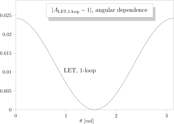
In Fig. 3, we plot the angular dependence of the one-loop correction. If the renormalization scale is chosen equal to the energy , the loop correction, and thus the angular dependence, is less than . Since the NLO correction is proportional to (compared with the LO amplitude proportional to ), it rapidly becomes important for . However, this mainly indicates the breakdown of the low-energy expansion at high energies.
We can transfer the scheme-dependent matching coefficients to the NLO counterterms, so the above result is reproduced by maintaining only the logarithmic terms in the amplitude,
| (28) |
and adding one-loop matching contributions to and ,
| (29) |
The renormalization scale dependence of these coefficients is given by
| (30) |
with some reference scale .
Isospin symmetry determines all individual scattering amplitudes in terms of the master amplitude :
| (31a) | ||||
| (31b) | ||||
| (31c) | ||||
| (31d) | ||||
| (31e) | ||||
Expanding the amplitudes in powers of the energy, the order- term is known as the low-energy theorem (LET) [41]:
| (32a) | ||||
| (32b) | ||||
| (32c) | ||||
| (32d) | ||||
| (32e) | ||||
These expressions are model-independent and depend just on the electroweak scale .
4.2 Resonances
In Sec. 3.2, we have introduced heavy resonances in weak-boson scattering. The interaction Lagrangians (10a–10e) induce couplings to vector bosons and to Goldstone bosons, which are related by electroweak gauge invariance, maintaining the GBET. Each resonance multiplet therefore contributes additional terms to the Goldstone scattering amplitude , which have poles at the appropriate locations. We do not yet include the resonance widths. The new contributions are
| (33a) | ||||
| (33b) | ||||
| (33c) | ||||
| (33d) | ||||
| (33e) | ||||
where .
Beyond the resonance location, for the exchange amplitude cancels the rise of the LET amplitude. This is the SM case. Otherwise, beyond the resonance all amplitudes rise with a power of . This implies again unitarity violation, which has to be cured by the unknown UV completion of the theory.
4.3 Eigenamplitudes
For the analysis of unitarity, we need the spin-isospin eigenamplitudes, i.e., scattering amplitudes for superpositions of states which scatter only into themselves. We first list the isospin eigenamplitudes
| (34a) | ||||
| (34b) | ||||
| (34c) | ||||
which can be decomposed into partial waves using Legendre polynomials,
| (35) |
where only for even. The coefficient functions are the spin-isospin eigenamplitudes. They are obtained by angular integration,
| (36) |
Below, we explicitly list the spin-isospin eigenamplitudes, treating LO, NLO, and resonances separately:
(a) The eigenamplitudes for the LO Lagrangian:
| (37) |
All other terms vanish at this order.
(b) The one-loop correction with its logarithmic angular dependence contains partial waves of arbitrary spin. We extract the leading logarithms , project out the partial waves and truncate the series at spin , which numerically is an excellent approximation. Adding the tree-level NLO coefficients, which should include their scheme-dependent and scale-dependent parts (29, 30), the real part of the result is
| (38a) | ||||
| (38b) | ||||
| (38c) | ||||
| (38d) | ||||
| (38e) | ||||
| (38f) | ||||
We note that the scale dependence of the parameters cancels the scale-dependence of the one-loop terms, as it should be the case. The results are shown in Fig. 4. While the loop correction is small below about , for higher energies it becomes important and, eventually, drastically changes the behavior. For instance, in there is a cancellation between the LO and NLO terms at . This clearly indicates the breakdown of the low-energy expansion.

(c) For the decomposition of resonance corrections, we define the following functions:
| (39a) | ||||
| (39b) | ||||
| (39c) | ||||
which we give explicitly in Appendix A.4. We obtain for the isosinglet scalar,
| (40a) | ||||||
| (40b) | ||||||
| (40c) | ||||||
the isoquintet scalar,
| (41a) | ||||||
| (41b) | ||||||
| (41c) | ||||||
the isotriplet vector,
| (42a) | ||||||
| (42b) | ||||||
| (42c) | ||||||
the isosinglet tensor,
| (43a) | ||||
| (43b) | ||||
| (43c) | ||||
| (43d) | ||||
| (43e) | ||||
| (43f) | ||||
and the isoquintet tensor,
| (44a) | ||||
| (44b) | ||||
| (44c) | ||||
| (44d) | ||||
| (44e) | ||||
| (44f) | ||||
The coefficient functions contain poles in as well as finite parts. The poles are confined to those combinations which correspond to the assignments of the resonances. Again, we truncate the partial-wave expansion at , so for each spin-isospin combination we only keep the leading and one subleading term.
4.4 Unitarization scheme
Elastic unitarity requires that the normalized eigenamplitudes
| (45) |
respect the Argand-circle condition
| (46) |
which can also be stated as
| (47) |
Computed in finite-order perturbation theory, or deduced from some model, the amplitude will usually fail this requirement. However, an arbitrary amplitude can be transformed into a unitary amplitude if we take the real part of and add as the imaginary part, i.e.,
| (48) | ||||
| (49) |
For the unnormalized eigenamplitudes , this can be rephrased as
| (50) |
With this prescription, a LET amplitude becomes
| (51) |
so instead of rising quadratically with energy, the absolute value of asymptotically approaches saturation, formally a resonance at infinity.
The K-matrix scheme transforms a simple-pole amplitude, , into Breit-Wigner form,
| (52) |
so it is an alternate implementation of Dyson resummation for s-channel particle exchange. If is not a constant but depends on energy, we get a Breit-Wigner resonance with -dependent width. In particular, the amplitude
| (53) |
is transformed into
| (54) |
Eq. (53) has the low-energy expansion
| (55) |
An expansion of this form can also be treated by the inverse-amplitude method (IAM) for unitarization [43]. The result is
| (56) |
which equals the Padé approximant, and precisely coincides with (54). We observe that, in the present context, the IAM or Padé unitarization scheme is a special case of the K-matrix scheme, where the low-energy expansion of the amplitude is identified with the low-energy tail of a single resonance. In QCD, where the meson dominates form factors at low energy, this turns out to be a valid assumption which leads to accurate high-energy extrapolations. In the electroweak case, physics may be different, and the actual (unitary) weak-boson scattering amplitudes need not follow the extrapolation of the K-matrix/IAM/Padé or any other given unitarization scheme.
In QCD, low-energy parameters can be computed, to good accuracy, by integrating out the resonance. This may also be the case for the leading resonances in electroweak interactions (we list the necessary formulas in Sec. 3.3), but there may well be extra contributions that can be assigned to further resonances, or to other physical effects. For this reason, we keep and as independent parameters in our implementation.
The detailed shape of resonances in weak-boson scattering may also differ from the (running-width) Breit-Wigner that our parameterization provides. However, the experimental resolution of weak-boson pair invariant masses at the LHC will be limited, so there is little hope for precise resonance scans. A parameterization in terms of mass and width, augmented by extra parameters which describe deviations in the low-energy tail, is sufficient.
Beyond a resonance peak, our expressions suggest a definite prediction, such as a new rise of the amplitude with a definite power of . We should emphasize that this is misleading: the behavior in this region is arbitrary and can only be modeled, introducing further parameters. However, any precise measurements of the high-energy tail of a heavy resonance will be challenging, if not impossible at the LHC. The only property of unitarized amplitudes that we really make use of is: that they do not exceed the unitarity limits.
4.5 Unitarized Amplitudes
In this section, we apply the unitarization scheme defined above to the generic parameterization of scattering amplitudes. Collecting everything, each eigenamplitude consists of a LO (LET) part, a NLO correction which includes the one-loop part and finite extra contributions to the parameters, and resonance terms:
| (57) |
which we write in the form
| (58) |
where is finite, and is proportional to (vector), or (scalar, tensor). According to the prescription in the previous section, the unitarized amplitude becomes
| (59) |
where the correction to the LET amplitude is given by
| (60) |
In Fig. 6 we draw the absolute values of the resulting unitarized eigenamplitudes, including the LET part (37). Since the resonances have definite spin and isospin quantum number assignments, each plot contains exactly one curve with a resonance, while the other curves are non-resonant. The resonance masses () have been set to , and the couplings to unity. The unitarization prescription smoothly cuts off the amplitudes, so their absolute values do not exceed the limit . Some of the amplitudes (e.g., ) contain terms rising like a power with the energy and eventually saturate this bound, while others (e.g., ) rise logarithmically at most, so at accessible energies they stay much below this limit.
For the scalar isosinglet , the choice corresponds to the SM with a heavy Higgs. In this case, unitarity is restored already by the scalar resonance exchange. Hence, as long as is below about , the asymptotic values of all stay below the limit of . At tree level, they are constants that depend on the ratio . This is slightly modified by loop corrections and by the unitarization prescription. For , the cancellations are incomplete, and the amplitudes behave in the same way as the other amplitudes.
Several of the curves exhibit a zero, which in the logarithmic plots manifests itself as a sharp down-pointing spike. In fact, in our parameterization this happens for all resonant amplitudes, with the exception of the SM Higgs case. The reason is negative interference between the resonant propagator and the contact term; the latter is necessary for satisfying the LET and rises with a higher power of the energy. For vector resonances, cancellation typically occurs at very high energies (above ), while for tensor resonances the effect is visible in the energy range that we have chosen for our plots. However, if such a zero occurs beyond the resonance mass, it should not be taken seriously, because in this range the amplitude contains further, undetermined contributions, and the energy behavior of the contact term as given by our formulae is not a prediction. Only if this zero appears below the resonance a dip should actually be expected. This is the case for in the presence of a scalar isoquintet.


The analytic behavior of the amplitudes is transparent if we plot the real part, which vanishes on a resonance. This is illustrated in Fig. 7. All curves cross zero at , the resonance mass. Beyond this, they rise and asymptotically approach zero again. This is the resonance at infinity generated by the unitarization procedure. The exception is the resonance which approaches a constant, since in this model (the SM) there is no unitarity problem.


For a concrete Monte-Carlo implementation, we need the unitarized amplitudes for physical states, e.g., , , etc. Therefore, we first translate the spin-isospin eigenamplitudes back into corrections to the isospin eigenamplitudes as functions of ,
| (61a) | ||||
| (61b) | ||||
| (61c) | ||||
The result is shown in Fig. 8. The plot clearly exhibits the characteristic angular dependence of the resonances with , respectively, while the continuum background that we have included is negligible for . The nonresonant part is important, however, to describe the off-peak amplitude behavior.
This, in turn, is translated into corrections to the individual scattering amplitudes,
| (62a) | ||||
| (62b) | ||||
| (62c) | ||||
| (62d) | ||||
| (62e) | ||||
Unitarization breaks crossing symmetry, since it is applied only in the s-channel. Explicitly, we obtain
| (63a) | ||||
| (63b) | ||||
| (63c) | ||||
| (63d) | ||||
| (63e) | ||||
Here, the coefficients functions are determined by decomposing the results from Sec. 4.3 according to (59) and inserting this into the unitarization formula (60).
4.6 Off-shell Implementation
For realistic calculations, we want to transform the unitarized Goldstone scattering amplitudes into matrix elements for off-shell weak-boson scattering. We first note that the complete SM without a Higgs and without anomalous couplings, already yields the LET result for weak-boson scattering. In order to avoid double-counting, we therefore have to remove the LET part from any extra contributions that we add to the theory. This is achieved by considering only the correction terms (62a–62e) instead of the complete unitarized amplitudes.
The chiral Lagrangian with NLO parameters (i.e., and ) provides an off-shell formulation for the low-energy effective theory. We can determine Feynman rules and compute complete matrix elements of fermion processes which include weak-boson interactions with anomalous couplings. The Feynman rules of four-boson couplings depend on and . In unitarity gauge, they are derived from the quartic gauge interactions
| (64) |
where the SM values of the couplings22 2 In these expressions, the numerical values of the electroweak gauge couplings and the weak mixing angle depend on the precise definition of the electroweak renormalization scheme. are given by
| (65) |
If we include the dependence on all five isospin-symmetric NLO chiral parameters (13a–13e), the deviations from the SM values are
| (66a) | ||||||
| (66b) | ||||||
| (66c) | ||||||
| (66d) | ||||||
We can now construct a generic off-shell parameterization of weak-boson scattering that corresponds to the unitary on-shell Goldstone scattering amplitudes (62a–62e). When the Feynman rule for a given quartic gauge vertex is inserted in a physical process, we replace the dependence on the constant parameters and by form factors which depend on . For and , this is straightforward: the two expressions and correspond to the two different interaction terms for () in the Lagrangian (64), so we simply can replace the constants and ( and ) by the full expressions (62a, 62d), respectively. For the other processes, this assignment cannot be done in the interaction Lagrangian, but it is obvious in the Feynman rule, where each term , , and corresponds to a definite combination of Lorentz factors.
As a first result, we can compute on-shell scattering amplitudes for physical and bosons. These combine the features of the chosen resonance model with SM effects such as photon and exchange. Since on-shell initial vector bosons cannot be prepared in practice, we defer this discussion to Appendix E.
Such an algorithm breaks crossing symmetry, but this is natural since the unitarization scheme already breaks crossing symmetry. In a practical implementation, for a given vertex we implement all possible orientations of the time arrow as alternatives, and determine the orientation that is actually realized when we insert the vertex into a physical process. This is straightforward to do for an automatic matrix-element generator.
Two sources for ambiguities appear in this construction. (i) The GBET relates Goldstone scattering amplitudes to weak-boson scattering amplitudes only in the high-energy limit, and only for longitudinal polarization. We do not specify couplings to transversal gauge bosons, which are not directly related to EWSB and formally subleading in the physics of strongly interacting weak bosons. Corrections to the GBET therefore can be computed only up to further free parameters. Keeping this in mind, we translate the Goldstone amplitudes to weak-boson amplitudes using the leading-order GBET.33 3 If we adopt the EWA, part of the difference w.r.t. complete amplitudes is formally of the same order as the GBET corrections. However, the EWA strongly affects kinematics and ignores a large set of irreducible background diagrams, so the numerical impact of this approximation for LHC analyses is much more important than model-dependent ambiguities in corrections to the GBET. (ii) Strictly speaking, the Mandelstam variables in form factors are defined for on-shell scattering of massless particles. , can be replaced by Lorentz factors which are unambiguous, but in the off-shell continuation, the subenergy squared is evaluated for massive off-shell bosons. This affects the unitarization corrections, but these are scheme-dependent anyway. Their main property – to cancel any unphysical rise of subamplitudes – is preserved off-shell. It also affects the location of resonance poles. However, as discussed in Sec. 3.2, off-shell effects in the latter are accounted for by higher-dimensional operators and translate into corrections to . Finally, we recall that the off-shell continuation of propagators is controlled by electroweak gauge invariance. We keep symmetry manifest in the gauge and fermion sectors by using covariant derivatives, so this is not an issue.
As a cross-check, we can compute fermion processes for the ordinary SM with a Higgs boson. In our parameterization, this is the chiral Lagrangian with and a resonance with . The form factors for the , , and vertices contain exactly the Higgs propagator factors that we would have obtained with the Higgs boson as an ordinary particle. In the -channel, the propagator pole turns out to be regularized by a running width , which is a sensible treatment of the width of a heavy Higgs boson in SM scattering amplitudes [44]. So, despite the fact that we have used the leading-order GBET, our off-shell formulation exactly reproduces the tree-level SM result, both on-shell and off-shell. The only missing parts are double-Higgs and Higgs-fermion couplings (see e.g. [45]), but those couplings do not contribute to the processes we are interested in.
5 LHC Processes
5.1 Monte-Carlo simulation
We have implemented our parameterization of vector-boson scattering in the multi-particle event generator WHIZARD [28, 29]. The program generates matrix elements for partonic processes via optimized helicity amplitudes while avoiding the redundancies inherent in a Feynman diagram expansion. These optimized matrix elements together with a highly efficient phase-space setup enable the simulation of six and eight-particle final states. WHIZARD contains the infrastructure for simulations of complex collider environments like structured beams, parton shower, and interfaces to fragmentation and hadronization.
As the starting point for the implementation in WHIZARD, we have chose the SM extension with anomalous three-boson and four-boson couplings which has been used for the simulation of anomalous triple and quartic gauge operators [20, 46, 47]. The algorithm for the symbolic generation of the matrix elements in WHIZARD, which is especially suited for the inclusion of beyond the Standard Model (BSM) physics [48], allows for the insertion of operators in specific time directions necessary by the crossing-symmetry breaking effects of the K-matrix unitarization prescription.
5.2 Comparison with the Effective approximation (EWA)
In fermion processes that contain weak-boson scattering (Fig. 1) the bosons that initiate the interaction are represented by their propagators with a spacelike momentum. The main contribution comes from the region with small virtuality, and we are interested in the region of large c.m. energy of the vector boson pair. In this region, the virtualities and the masses of the vector bosons induce only small corrections to the amplitude, so the initial vector bosons can be treated as approximately on-shell.
We can thus approximate the dominant Feynman graphs by a convolution of massless splitting (of the initial quark into a quark and a vector boson) with the vector-boson interaction, which is called effective approximation (EWA) [25]:
| (67) |
This has to be convoluted with the quark structure functions to yield the cross section for the initial state.
Eq. (67) contains integrations over , the energy fractions of the vector bosons that are radiated from the initial quarks, and a sum over vector-boson helicities. In contrast to the analogous Weizsäcker-Williams approximation for photons, there is a longitudinal polarization direction in addition to the two transversal polarization directions. Explicitly, the structure functions are
| (68a) | ||||
| (68b) | ||||
| (68c) | ||||
with . The vector and axial couplings for a fermion branching into a are
| (69) |
For emission, this is replaced by
| (70) |
where is the fermion isospin, and its charge.
These structure functions depend on a transverse-momentum cutoff . The kinematical limit for the cutoff is
| (71) |
In the derivation of (68a–68c), one integrates over under the assumption that it is small compared to the subprocess energy, so the subprocess cross section does not depend on it. For the longitudinal structure function that we are most interested in, this can be justified because the limit is finite. This structure function is concentrated near . The transverse structure functions have a logarithmic divergence in , so the cutoff is needed there. This already suggests that the EWA is more reliable for longitudinal than for transversal vector bosons.


In Fig. 9, we display the structure functions of and bosons, separately for positive, longitudinal, and negative helicity. The emitting quark has been chosen to be an up-type quark; for down-type quarks or electrons the curves have to be renormalized according to the respective charges. For antiquarks or positrons, the transverse polarizations have to be interchanged. The plots illustrate the fact that emission of a or , in particular at high energies, is more likely for a transversally polarized vector boson. In effect, the production of longitudinally polarized pairs which couple to the symmetry-breaking sector is suppressed compared to this irreducible background.


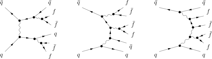
Fig. 11 exemplifies the differences between the exact result for processes which contain resonant weak-boson scattering. To make a meaningful comparison, we first recall that in the EWA the initial vector bosons are on-shell, while in the exact process they are off shell. The on-shell amplitudes have a Coulomb singularity due to photon and exchange. In particular, an on-shell cross section with photon exchange is infinite, while exchange yields a Coulomb peak proportional to . Here, is the c.m. energy of the vector-boson subsystem, equal to the invariant mass squared of the outgoing vector bosons. To reduce this effect which in the exact result is regulated by the vector-boson virtuality, we cut the of the outgoing vector bosons at .
A particular choice of this cut allows us to approximate the high-energy end of the distribution for the SM with a heavy Higgs (Fig. 11, top) quite well [25]. This is misleading, however: with the same cut, the prediction of the tensor resonance case (Fig. 11, lower left) with its unitarity saturation beyond the peak is considerably worse. If we are looking at instead of , the EWA background undershoots the exact value (Fig. 11, lower right). More importantly, while the peak can be approximated up to better than a factor , the background is predicted with less accuracy. Since cannot be reconstructed experimentally (apart from final states), so sideband subtraction is not possible, this significantly affects the analysis.
Part of the deviation is due to the kinematical simplifications inherent in the derivation, which can be improved in principle [49, 18]. Unfortunately, this only marginally improves the EWA, since the main error comes from the existence of irreducible background diagrams for on-shell vector boson pair + jets production, and additional irreducible background for the complete six-fermion process, cf. Fig. 11, which cannot be accounted for in this way. Off-shell, those background diagrams are connected to the signal diagrams by gauge invariance and cannot be neglected: simply omitting them would disrupt detailed cancellations, similar to the familiar s/t-channel cancellation in pair production [50].
5.3 Complete Simulation
The implementation of the off-shell continued amplitudes in the Monte-Carlo generator WHIZARD allows us to get rid of the EWA and to simulate event samples for the complete process , where the four additional fermions are the decay products of the vector bosons, or come from the irreducible background. Using, e.g., PYTHIA for parton showering and fragmentation, this results in physical LHC events that can be analyzed by detector simulation and eventually compared to real data.
For illustration, in Fig. 12 we present the result of a parton-level simulation of scattering, using complete six-fermion matrix elements. In these plots, we compare the effect of a vector resonance with the nonresonant (unitarized) LET model, which serves as a reference model for the higgsless case. In the four-lepton invariant mass, the resonance is clearly visible. However, this quantity is not an observable. The azimuthal distance of the two decay leptons is observable; there, vector-resonance exchange in - and -channel leads to a significant excess.


A realistic study would be based on a sum over all possible final states with parton shower and hadronization, using cuts and distributions in observable quantities. Furthermore, it would include a complete account of background and detector effects. A cut-based analysis strategy was proposed in Refs. [8, 9]. An ATLAS study that makes use of the parameterization of the present paper is currently under way [51].
6 Summary and Conclusions
We have described a generic approach to extrapolating vector-boson scattering into the energy range where no perturbative predictions exist. Nontrivial features of the amplitudes are possible, which will likely appear as resonances. In addition to the classical alternative of a heavy scalar-isoscalar (Higgs) or a vector-isovector (technirho or ) resonance, we account for scalar-isotensor resonances which are present in extended models, and for tensor resonances that could, for instance, be associated with gravity in extra dimensions. Furthermore, we connect the model-dependent part to the model-independent low-energy effective theory and keep this relation transparent in the implementation. Unitarization of the on-shell amplitudes avoids the problem of unphysical behavior at the highest energies that plagues a naive tree-level approach.
Our approach is economical in the number of free parameters, but intended as a sufficiently general description of those energy regions where the LHC will have sensitivity. If necessary, refinements of the models, such as recurring resonances or more exotic behavior of the amplitudes, are straightforward to add. The resulting amplitudes are translated into effective form-factors for vector-boson vertices in unitarity gauge. This allows for an implementation in universal Monte-Carlo event generators, which we have realized for the case of the WHIZARD event generator.
While the leading electroweak loop corrections for vector-boson scattering are included, QCD corrections are not yet implemented. These have been considered in Ref. [52] and should be combined with the effects modeled by our approach.
With the event generator at hand, model-independent studies and analyses of vector-boson scattering, both in SM extensions and in Higgsless models, become feasible. No approximations beyond those inherent in the modeling are involved, as it is essential for unbiased data analysis. A particular feature of our implementation is the smooth transition to the SM case (with a Higgs boson) or, alternatively, to a featureless LET model of strong scattering without resonances, respecting unitarity. In data analysis, the signal can be defined as the deviation with respect to either one of those reference models.
Acknowledgments
We thank Michael Kobel, Wolfgang Mader, Markus Schumacher and especially Jan Schumacher for their fruitful discussions and helpful comments during the development of this work. JR was partially supported by the Bundesministerium für Bildung und Forschung, Germany, under Grant No. 05HA6VFB. During its early stage this research was supported by the Helmholtz-Gemeinschaft under Grant No. VH-NG-005.
Appendix A Conventions and algebra
A.1 algebra
Throughout this paper, we use boldface notation for objects that are defined in the adjoint of , e.g.,
| (72) |
with the Pauli matrices (), and summation over understood.
For describing isospin quintet resonances, we introduce tensor products of Pauli matrices:
| (73) | ||||
| (74) | ||||
| (75) | ||||
| (76) | ||||
| (77) |
These are normalized:
| (78) |
Isospin singlet:
| (79) |
Tracing this with something else gives
| (80) |
in particular
| (81) |
Furthermore we need:
| (82) |
A.2 Goldstone bosons and Gauge fields
We define the Goldstone scalar triplet or, alternatively, such that
| (83) |
and . Contractions:
| (84) | ||||
| (85) |
The Higgs-field matrix is given by
| (86) |
The covariant derivative of the Higgs field is
| (87) |
Unitary gauge would mean , i.e., . Herewith, we define the vector field
| (88) |
which is in the adjoint representation of , and is a linear combination of Pauli matrices. Hence, . Note that is antihermitian, .
Gauge fields for the electroweak and strong interactions are defined such that they transform under as ,
| (89) | ||||
| (90) |
furthermore there is the QCD gauge field .
In the gaugeless limit, the expansion in terms of Goldstone fields is . Expressing this in terms of charge eigenstates, we derive
| (91) | ||||
| and thus | ||||
| (92) | ||||
Hence,
| (93) |
In the notation used for couplings to isospin quintets, we have
| (94) |
And,
| (95) |
A.3 Tensor Fields
A massive tensor field is subject to the conditions
| (96) |
Its spin sum is given by
| (97) |
where
| (98) |
The free Lagrangian is
| (99) |
where the kinetic part corresponds to the spin sum (97).
A.4 Integrals in spin-isospin eigenamplitudes
To get compact expressions for the spin-isospin eigenamplitudes, we define the following integrals:
| (100a) | ||||
| (100b) | ||||
| (100c) | ||||
The integrals over are times those over .
Explicit expressions for these integrals are:
| (101a) | ||||
| (101b) | ||||
| (101c) | ||||
| (101d) | ||||
| (101e) | ||||
| (101f) | ||||
| (101g) | ||||
| (101h) | ||||
Appendix B Feynman rules for scalar and tensor resonances
We briefly summarize the Feynman rules for scalar and tensor resonances that derive from the interaction Lagrangians (10a)-(10e). The s in this section are the momenta of the Goldstone bosons.
Scalar isoscalar:
| (102) |
Scalar isotensor:
| (103) | ||||||
| (104) |
For the Feynman rules of the tensor resonances we use the symbol to get (momenta incoming).
Tensor isoscalar:
| (105) |
Tensor isotensor:
| (106) | ||||||
| (107) |
Note that taking the conditions on the tracelessness as well as the transversality not necessarily demands the coupling of the tensor resonance to a conserved current (like the energy-momentum tensor) which leads to the same Feynman rules as in [53]. The constraint of the LET on the other hand results in an (off-shell continued) amplitude that is identical to the one of a massive graviton resonance.
Appendix C Vector Resonance Exchange
Heavy vector resonances have been studied many times in the literature, and various different formalisms describe their interactions with the SM particles. In this section, we demonstrate the equivalence of some popular approaches. In particular, we look at the correction to the amplitude for Goldstone-Goldstone scattering which via the GBET and spin/isospin symmetry yields the leading term for all channels of quasi-elastic scattering, . Since we maintain manifest gauge invariance by using covariant derivatives, the GBET holds in any formalism that we describe. If desired, this can be verified by switching to unitarity gauge and computing the scattering amplitudes directly.
We ignore couplings to fermion currents, which generically will be present and sizable. While such couplings get shifted by some of the transformations described below, in our model-independent approach they are considered as independent parameters which are determined by independent measurements. The shifts of fermion couplings induced by reparameterizations merely change a set of undetermined parameters into another set of undetermined parameters, so for our purposes there is no need to calculate them. However, in the context of a specific model, one should always treat fermionic and bosonic sectors together when applying reparameterizations [54]. A specific example for this in the context of Little Higgs models can be found in [55].
- 1.
We use the representation with the Goldstone field and introduce the resonance as a vector field in the iso-triplet representation. The Goldstone kinetic term is
(108) and can be expanded up to second order as
(109) (110) The interaction Lagrangian is
(111) Ignoring gauge fields, we carry out the expansion up to third order:
(112) (113) (114) leading to the corresponding Feynman rules
(115) (116) (117) 
Figure 13: Feynman graphs for : contact term from the non-linear Lagrangian leading to the LET on the left, resonance - and -channel exchange in the middle, and contact terms from mixing on the right. The resulting Feynman graphs for are shown in Fig. 13. There is a Goldstone contact interaction from the Goldstone kinetic term; this yields the low-energy theorem (LET) . Resonance exchange adds - and -channel contributions,
(118) which in the limit become . Furthermore, there are contributions where the resonance mixes with the external Goldstone scalar, either as an external wave-function correction, or with the coupling to three scalars. In both graph types the resonance pole cancels, so they are additional contact terms proportional to . In unitarity gauge, this translates into a correction to masses and interactions.
The appearance of a contact term looks like a violation of the LET. However, the measured value of (e.g., as extracted from pole data) includes those additional contributions, so they merely renormalize a fictitious bare value. This renormalization can be made explicit by adding a counterterm to the interaction Lagrangian, which by power counting and symmetries must be of the form with an appropriate prefactor . In effect, expressed in terms of the observed scale , the LET holds, and the vector-exchange amplitude is given by
(119) which vanishes as as .
- 2.
In the previous paragraph, the vector resonance was coupled to bosons by a mass mixing term, . Alternatively, we could couple it by a kinetic mixing term,
(120) where the resonance “field strength” is with the covariant derivative in the adjoint representation. Partial integration gives
(121) Here, we can apply the field equation
(122) to obtain
(123) as before, so we get the same scattering amplitude. Using the equations of motion is precisely an application of the UET.
- 3.
In the CCWZ formalism [31], the elementary building block is with . From , we can construct a vector and an axial vector field,
(124) Under , these transform like a gauge field and a matter field, respectively,
(125) is related to the vector current that we have used in our previous formulation: . We just have to redefine to obtain
(126) so a matter field coupled to the axial vector yields the same scattering amplitude again.
- 4.
Alternatively, we can couple to the vector field by assigning to it a gauge-field transformation law under ,
(127) so the leading invariant term containing is
(128) The expansion of is even in the number of Goldstone fields. Therefore, in this expression, the last term is the mass, the second term yields the and couplings, and the first term is a contact term. Note that the gauge coupling is proportional to . The resulting amplitude is again (119), this time without the need for renormalizing .
- 5.
The BESS model [6] has a similar setup. Instead of gauging just , we can extend the local symmetry by an extra local, nonlinearly realized . This results in two vector isotriplets, which can be combined to a vector and an axial vector isotriplet, respectively. Only the vector couples to longitudinal pairs, and the amplitude (119) can be derived as before.
The different formalisms for coupling vector resonances all result in the same scattering amplitude. This is not surprising since this amplitude is completely determined by spin and isospin conservation together with the LET. In order to give the CCWZ interpretation of the vector resonance as a gauge field (in contrast to a generic matter field) a physical meaning, we would have to measure triple couplings, analogous to the LEP2 measurements of triple gauge couplings. Unfortunately, such measurements are beyond the reach of LHC.
Appendix D Specific Models
In the literature, a variety of “benchmark” models has been formulated that test weak-boson scattering. In this section, we relate some of them to our parameterization:
- 1.
The SM. As discussed in the main text, for the scalar resonance model precisely reproduces SM Higgs exchange. Alternatively, one can switch to the default SM implementation (in WHIZARD) without extra resonances.
- 2.
Scalar resonances. Refs. [8, 9] introduce a collection of models, among them two with a scalar resonance (“” and “chirally coupled scalar”). The latter model is identical to our scalar resonance parameterization. The model is essentially a special case of this with fixed mass and width; the only distinction is a logarithmic cutoff-dependent modification, which manifests itself beyond the resonance. This detail is unlikely to be detectable at the LHC.
- 3.
- 4.
Padé/IAM unitarization model.
As discussed in Sec. 4.5, this scheme is a special case of the K-matrix scheme as defined in the present paper. For a given combination we use Eqs. (38a, 38c, 38e) to determine the NLO correction to the three amplitudes , , and which without correction would violate unitarity. Then, we can use (56) to identify scalar, vector, and tensor resonance masses and widths. If we neglect the loop corrections in (38a–38e), we obtain
(129a) (129b) (129c) where we have to define a renormalization scheme and fix the scale . Note that the tensor-resonance parameters are unphysical. This is due to the negative sign of in Eq. (37). This model ignores the possibility of isotensor resonances or .
Appendix E On-shell vector boson scattering
In this section we summarize the plots for “partonic” scattering of spin-averaged and summed vector bosons. In all these pictures, the EW gauge bosons are treated on-shell, hence the cross sections start when the physical or threshold is reached. Since we did not switch off the electromagnetic coupling in those plots, we applied a cut of 15 degrees around the beam axis to cut out the Coulomb scattering part. Fig. 14 shows in the upper line the SM with a 120 GeV Higgs on the left and a heavy 1 TeV on the right. Unitarity is preserved in those cases because of the (-channel) Higgs exchange. Besides the dominant resonance for a heavy Higgs, the amplitudes show a saturation for the high-energy tails which starts again violating partial-wave unitarity for 1.2, 3.5, and 1.7 TeV for the isospin channels, respectively. Completely removing the Higgs as in the middle line of 14 leads to a rise of the amplitudes (and hence the cross sections) with (the process is absent in that case). Switching on the -matrix unitarization damps the amplitudes back to the Argand circle, thereby restoring unitarity. This happens for the above mentioned values for the corresponding isospin eigenamplitudes. In the lower line of Fig. 14, the case of the LET extended by nonzero values for the parameters and are shown, on the left the badly diverging case without unitarization, and the K-matrix unitarized case on the right.
In Fig. 15 we show the cross sections for the five different vector boson scattering processes with the presence of the five isospin-allowed resonances mentioned in the text. and contain all three isospin eigenamplitudes, hence show a resonance in all channels except for the vector resonance case where it is forbidden by the Yang-Landau theorem. The amplitude does not have isoscalar resonances, while the amplitude allows only isotensor resonances. Finally, contains all resonances.


References
- [1] R. S. Chivukula, A. G. Cohen and K. D. Lane, Nucl. Phys. B 343, 554 (1990).
- [2] A. Dobado, A. Gomez-Nicola, A. Maroto and J. R. Pelaez, Effective lagrangians for the standard model, N.Y., Springer-Verlag, 1997. (Texts and Monographs in Physics);
- [3] C. T. Hill and E. H. Simmons, Phys. Rept. 381, 235 (2003) [Erratum-ibid. 390, 553 (2004)] [arXiv:hep-ph/0203079].
- [4] W. Kilian, Springer Tracts Mod. Phys. 198, 1 (2003).
- [5] M. S. Chanowitz and M. K. Gaillard, Nucl. Phys. B 261, 379 (1985).
- [6] R. Casalbuoni, S. De Curtis, D. Dominici, and R. Gatto, Phys. Lett. B155 (1985) 95; Nucl. Phys. B282 (1987) 235; R. Casalbuoni et al., Phys. Lett. B 349, 533 (1995); R. Casalbuoni et al., Phys. Rev. D 53, 5201 (1996).
- [7] S. Weinberg, Phys. Rev. D13 (1976) 974; Phys. Rev. D19 (1979) 1277; L. Susskind, Phys. Rev. D20 (1979) 2619.
- [8] J. Bagger et al., Phys. Rev. D 49 (1994) 1246 [arXiv:hep-ph/9306256].
- [9] J. Bagger et al., Phys. Rev. D 52 (1995) 3878 [arXiv:hep-ph/9504426].
- [10] S. N. Gupta, J. M. Johnson, G. A. Ladinsky and W. W. Repko, Phys. Rev. D 53 (1996) 4897 [arXiv:hep-ph/9603416].
- [11] A. Dobado, M. J. Herrero, J. R. Pelaez, E. Ruiz Morales and M. T. Urdiales, Phys. Lett. B 352 (1995) 400 [arXiv:hep-ph/9502309]; A. Dobado and M. T. Urdiales, Z. Phys. C 71 (1996) 659 [arXiv:hep-ph/9502255]; J. R. Pelaez, Phys. Rev. D 55 (1997) 4193 [arXiv:hep-ph/9609427]; A. Dobado, M. J. Herrero, J. R. Pelaez and E. Ruiz Morales, Phys. Rev. D 62 (2000) 055011 [arXiv:hep-ph/9912224].
- [12] ATLAS collab., CERN-LHCC-99-15 (1999).
- [13] A. S. Belyaev, O. J. P. Eboli, M. C. Gonzalez-Garcia, J. K. Mizukoshi, S. F. Novaes and I. Zacharov, Phys. Rev. D 59, 015022 (1999); S. Haywood et al., arXiv:hep-ph/0003275.
- [14] J. M. Butterworth, B. E. Cox and J. R. Forshaw, Phys. Rev. D 65 (2002) 096014 [arXiv:hep-ph/0201098].
- [15] D. Green, arXiv:hep-ex/0309031.
- [16] M. Fabbrichesi and L. Vecchi, Phys. Rev. D 76 (2007) 056002 [arXiv:hep-ph/0703236].
- [17] V. D. Barger, K. m. Cheung, T. Han and R. J. N. Phillips, Phys. Rev. D 52 (1995) 3815 [arXiv:hep-ph/9501379]; T. Han, Int. J. Mod. Phys. A11 (1996) 1541;
- [18] E. Boos, H. J. He, W. Kilian, A. Pukhov, C. P. Yuan and P. M. Zerwas, Phys. Rev. D 57, 1553 (1998); Phys. Rev. D 61, 077901 (2000); W. Kilian, Int. J. Mod. Phys. A15 (2000) 2387. J. A. Aguilar-Saavedra et al. [ECFA/DESY LC Physics Working Group], arXiv:hep-ph/0106315.
- [19] F. Gangemi, G. Montagna, M. Moretti, O. Nicrosini and F. Piccinini, arXiv:hep-ph/0001065.
- [20] M. Beyer, W. Kilian, P. Krstonošić, K. Mönig, J. Reuter, E. Schmidt and H. Schröder, Eur. Phys. J. C 48 (2006) 353 [arXiv:hep-ph/0604048].
- [21] C. Csaki, C. Grojean, H. Murayama, L. Pilo and J. Terning, Phys. Rev. D 69 (2004) 055006 [arXiv:hep-ph/0305237]; C. Csaki, C. Grojean, L. Pilo and J. Terning, Phys. Rev. Lett. 92 (2004) 101802 [arXiv:hep-ph/0308038]; Y. Nomura, JHEP 0311 (2003) 050 [arXiv:hep-ph/0309189]; G. Burdman and Y. Nomura, Phys. Rev. D 69 (2004) 115013 [arXiv:hep-ph/0312247].
- [22] R. Sekhar Chivukula, D. A. Dicus and H. J. He, Phys. Lett. B 525 (2002) 175 [arXiv:hep-ph/0111016]; R. S. Chivukula and H. J. He, Phys. Lett. B 532 (2002) 121 [arXiv:hep-ph/0201164]; R. S. Chivukula, D. A. Dicus, H. J. He and S. Nandi, Phys. Lett. B 562 (2003) 109 [arXiv:hep-ph/0302263].
- [23] H. Davoudiasl, J. L. Hewett, B. Lillie and T. G. Rizzo, Phys. Rev. D 70 (2004) 015006 [arXiv:hep-ph/0312193].
- [24] A. Birkedal, K. Matchev and M. Perelstein, Phys. Rev. Lett. 94 (2005) 191803 [arXiv:hep-ph/0412278].
- [25] M. S. Chanowitz and M. K. Gaillard, Phys. Lett. B 142, 85 (1984); G. L. Kane, W. W. Repko and W. B. Rolnick, Phys. Lett. B 148, 367 (1984). Nucl. Phys. B 249, 42 (1985); J. Lindfors, Z. Phys. C 28, 427 (1985); J. F. Gunion, J. Kalinowski and A. Tofighi-Niaki, Phys. Rev. Lett. 57, 2351 (1986).
- [26] S. Weinberg, Phys. Rev. 166 (1968) 1568; S. Weinberg, Physica A 96, 327 (1979).
- [27] T. Appelquist and C. W. Bernard, Phys. Rev. D 22, 200 (1980); A. C. Longhitano, Phys. Rev. D 22, 1166 (1980); Nucl. Phys. B188 (1981) 118; T. Appelquist and G. H. Wu, Phys. Rev. D 48, 3235 (1993) [arXiv:hep-ph/9304240].
- [28] http://whizard.event-generator.org; W. Kilian, T. Ohl, J. Reuter, arXiv:0708.4233 [hep-ph]; W. Kilian, LC-TOOL-2001-039.
- [29] T. Ohl, hep-ph/0011243; M. Moretti, T. Ohl, J. Reuter, hep-ph/0102195; J. Reuter, hep-th/0212154.
- [30] B. Lee, C. Quigg and H. Thacker, Phys. Rev. Lett. 38 (1977) 883; Phys. Rev. D16 (1977) 1519; D. Dicus and V. Mathur, Phys. Rev. D7 (1973) 3111.
- [31] S. R. Coleman, J. Wess and B. Zumino, Phys. Rev. 177 (1969) 2239; S.R. Coleman, J. Wess, and B. Zumino, Phys. Rev. 177 (1969) 2239; C. G. Callan, S. R. Coleman, J. Wess and B. Zumino, Phys. Rev. 177, 2247 (1969).
- [32] J. Gasser and H. Leutwyler, Ann. Phys. (N.Y.) 158 (1984) 142; Nucl. Phys. B250 (1985) 465.
- [33] D. Ross and M. Veltman, Nucl. Phys. B95 (1975) 135; M. Veltman, Act. Phys. Pol. B8 (1977) 475; Nucl. Phys. B123 (1977) 89; P. Sikivie, L. Susskind, M. Voloshin, and V. Zakharov, Nucl. Phys. B173 (1980) 189.
- [34] L. Randall and R. Sundrum, Phys. Rev. Lett. 83 (1999) 3370 [arXiv:hep-ph/9905221].
- [35] N. Arkani-Hamed, A. G. Cohen, E. Katz and A. E. Nelson, JHEP 0207, 034 (2002) [arXiv:hep-ph/0206021];
- [36] C.E. Vayonakis, Lett. Nuovo Cim. 17 (1976) 383; G. J. Gounaris, R. Kögerler and H. Neufeld, Phys. Rev. D 34, 3257 (1986); Y.-P. Yao and C.-P. Yuan, Phys. Rev. D38 (1988) 2237; J. Bagger and C. Schmidt, Phys. Rev. D34 (1990) 264.
- [37] R. Haag, Phys. Rev. 112 (1958) 669; H.J. Borchers, Nuovo Cim. 25 (1960) 270; D. Ruelle, Helv. Phys. Acta 35 (1962) 34; J.M. Cornwall, D.N. Levin, and G. Tiktopoulos, Phys. Rev. D10 (1974) 1145, Erratum D11 (1975) 972; M.C. Bergère and Y.-M.P. Lam, Phys. Rev. D13 (1976) 3247; P. Breitenlohner and D. Maison, Commun. Math. Phys. 52 (1977) 11, 39, 55.
- [38] F. Larios and C. P. Yuan, Phys. Rev. D 55 (1997) 7218 [arXiv:hep-ph/9606397].
- [39] O. Cheyette and M. K. Gaillard, Phys. Lett. B 197, 205 (1987).
- [40] S. Dawson and S. Willenbrock, Phys. Rev. D 40, 2880 (1989).
- [41] S. Weinberg, Phys. Rev. Lett. 17 (1966) 616; M.S. Chanowitz, M. Golden, and H. Georgi, Phys. Rev. D36 (1987) 1490.
- [42] S.N. Gupta, Quantum Electrodynamics, Gordon and Breach, 1981; M. S. Chanowitz, Phys. Rept. 320, 139 (1999)
- [43] A. Dobado and J. R. Pelaez, Phys. Rev. D 56, 3057 (1997) [arXiv:hep-ph/9604416].
- [44] W. Kilian and K. Riesselmann, Phys. Rev. D 58, 053004 (1998) [arXiv:hep-ph/9801265].
- [45] C. Delaunay, C. Grojean and J. D. Wells, JHEP 0804, 029 (2008) [arXiv:0711.2511 [hep-ph]]; G. F. Giudice, C. Grojean, A. Pomarol and R. Rattazzi, JHEP 0706, 045 (2007) [arXiv:hep-ph/0703164].
- [46] W. Menges, LC-PHSM-2001-022.
- [47] W. Kilian and J. Reuter, hep-ph/0507099; S. Kraml et al., arXiv:hep-ph/0608079;
- [48] T. Ohl, J. Reuter, Eur. Phys. J. C 30, 525 (2003); Phys. Rev. D 70, 076007 (2004); K. Hagiwara et al., Phys. Rev. D 73, 055005 (2006); J. Reuter et al., arXiv:hep-ph/0512012; W. Kilian, D. Rainwater, J. Reuter, Phys. Rev. D 71, 015008 (2005); Phys. Rev. D 74, 095003 (2006) W. Kilian, J. Reuter, T. Robens, Eur. Phys. J. C 48, 389 (2006); T. Robens, J. Kalinowski, K. Rolbiecki, W. Kilian, J. Reuter, arXiv:0803.4161.
- [49] P. W. Johnson, F. I. Olness and W. K. Tung, Phys. Rev. D 36 (1987) 291.
- [50] E. Accomando, A. Ballestrero, A. Belhouari and E. Maina, Phys. Rev. D 74 (2006) 073010 [arXiv:hep-ph/0608019].
- [51] J. Schumacher et al., in preparation.
- [52] B. Jäger, C. Oleari and D. Zeppenfeld, JHEP 0607 (2006) 015 [arXiv:hep-ph/0603177]; Phys. Rev. D 73 (2006) 113006 [arXiv:hep-ph/0604200]; G. Bozzi, B. Jäger, C. Oleari and D. Zeppenfeld, Phys. Rev. D 75 (2007) 073004 [arXiv:hep-ph/0701105].
- [53] T. Han, J. D. Lykken and R. J. Zhang, Phys. Rev. D 59, 105006 (1999) [arXiv:hep-ph/9811350].
- [54] A. Nyffeler and A. Schenk, Phys. Rev. D 62 (2000) 113006 [arXiv:hep-ph/9907294].
- [55] W. Kilian and J. Reuter, Phys. Rev. D 70 (2004) 015004 [arXiv:hep-ph/0311095].
- [56] R. Casalbuoni, S. De Curtis and D. Dominici, Phys. Lett. B 403 (1997) 86 [arXiv:hep-ph/9702357].