Simple Glass Models and Their Quantum Annealing

Consider $N$ Pauli spins $\sigma$ in a transverse field $\Gamma$ with the Hamiltonian:

where ${\cal}E(\{{\sigma^{z}\}})$ is a function that takes $2^{N}$ different values for the $2^{N}$ configurations of the $N$ spins. These values are taken randomly from a Gaussian distribution of zero mean and variance $N/2$, as in the REM [7]. A concrete implementation is ${\cal}E(\{{\sigma^{z}\}})=\lim_{\begin{subarray}{c}p\to\infty\end{subarray}}\sum_{i_{1},...,i_{p}}J_{i_{1},...,i_{p}}{\color[rgb]{0,0,0}{\sigma^{z}_{i_{1}}\cdots\sigma^{z}_{i_{p}}}}$, where the $J_{i_{1},...,i_{p}}$ are random Gaussian variables. In the $\sigma^{z}$ representation ${\cal{H}}$ is a $2^{N}\times 2^{N}$ matrix whose diagonal entries are the $2^{N}$ classical energies. The matrix elements of ${\cal{H}}_{0}^{\alpha\alpha}=E_{\alpha}^{{\color[rgb]{0,0,0}{\rm REM}}}$ and ${\cal{H}}_{0}^{\alpha\neq\beta}=0$, while $V_{\alpha\beta}=1$ if $\alpha$ and $\beta$ are two configurations that differ by a single spin flip and zero otherwise. ${\cal{H}}$ is sparse and can be studied numerically rather efficiently even for large matrix sizes using Arnoldi and Ritz methods [15]

The model is trivially solved in the limit $\Gamma\to 0$ and $\Gamma\to\infty$. For $\Gamma=0$, we recover the classical REM with $N$ Ising spins and $2^{N}$ configurations, each corresponding to an energy level $E_{\alpha}$ [7]: Call $n(E)$ the number of energy levels belonging to the interval $(E,E+dE)$; its average over all realizations is easily computed: $\overline{n(E)}=2^{N}P(E)\propto e^{N\left(\ln\!2-E^{2}/N^{2}\right)}=e^{Ns(E/N)}$, where $s(e)=\ln\!2-e^{2}$ (with $e=E/N$). There is therefore a critical energy density $e_{0}=-\sqrt{\ln\!2}$ such that, if $e<e_{0}$, then with high probability there are no configurations while if $e>e_{0}$ the entropy density is finite. A transition between these two regimes arises at $\frac{1}{T_{c}}=\frac{ds(e)}{de}\big|_{e_{0}}=2\sqrt{\ln\!2}$ and the thermodynamic behavior follows: (i) For $T<T_{c}$, $f_{\rm REM}=-\sqrt{\ln\!2}$ and the system is frozen in its lowest energy states. Only a finite number of levels (and only the ground state at $T=0$) contribute to the partition sum. The energy gap between them is finite. (ii) For $T>T_{c}$, $f_{\rm REM}=-\frac{1}{4T}-T\ln\!2$; exponentially many configurations contribute to the partition sum.

In the opposite case of very large values of $\Gamma$, the REM contribution to the energy can be neglected. In the $\sigma^{x}$ basis, we find $N$ independent classical spins in a field $\Gamma$; the entropy density is just given by the log of a binomial distribution between $-\Gamma N$ and $+\Gamma N$ and the free-energy density is $f_{\rm para}=-T\ln\!2-T\ln\!\left(\cosh\!\Gamma/T\right)$.

What happens between these two extreme cases? The perhaps surprising answer for the thermodynamics is nothing. At low value of $\Gamma$, the free-energy density is that of the classical REM, while for larger values it jumps to the quantum paramagnetic (QP) value $f_{\rm QP}$; a first-order transition separates the two different behaviors at the value $\Gamma$ such that $f_{\rm REM}=f_{\rm QP}$ (see center panel of Fig. 1). This can be easily understood using Rayleigh-Schrödinger perturbation theory [16, 17].

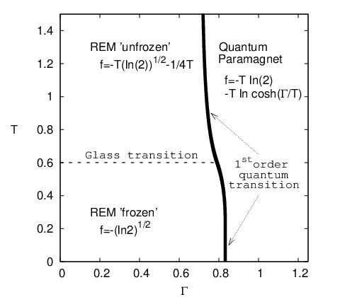
Consider the set of eigenvalues $E_{k}$ and eigenvectors $|k\rangle$ of the unperturbed REM, when $\Gamma=0$. The series for a given perturbed eigenvalue $E_{i}(\Gamma)$ reads

where the projector $Q=\sum_{\begin{subarray}{c}k\neq i\end{subarray}}|k\rangle\langle k|$ so that

Since $V_{ij}\neq 0$ if and only if $i$ and $j$ are two configurations that differ by a single spin flip, odd order terms do not contribute in Eq. (1) as one requires an even number of flips to come back to the initial configuration in the sums. Noting that $\sum_{k\neq n}|V_{nk}|^{2}$ reduces to a sum over the $N$ levels connected to $E_{i}$ by a single spin flip, one obtains, starting from an extensive eigenvalue [$E_{i}=O(N)$], that

where we have used that the $E_{k}$ are random and typically of order $\sqrt{N}$. Higher $n$th orders are computed in the same spirit and are found to be $O(N^{n/2-1})$. Therefore, to all (finite) orders, we have

This analytic result compares well with a numerical evaluation of the eigenvalues (left panel of Fig. 1). Note that the energy density of all extensive levels is independent of $\Gamma$ to leading order in $N$ as are hence $s(e)$ and $f(T)$.

The expansion can also be performed using $\Gamma V$ as a starting point and ${\cal H}_{0}$ as a perturbation. Consider the ground state with eigenvalue $E_{0}(\Gamma)$ and the unperturbed ground state with $E_{0}^{V}(\Gamma)=-\Gamma N$. In the base corresponding to the eigenvalues of $\Gamma V$, we find

The first-order term gives $\sum_{{\color[rgb]{0,0,0}{\alpha=1}}}^{2^{N}}E^{\rm REM}_{\color[rgb]{0,0,0}{\alpha}}{\color[rgb]{0,0,0}{|v_{\alpha}|^{2}}}$. Since the energies of the REM are random and uncorrelated with $v_{\color[rgb]{0,0,0}{\alpha}}$ this sums to $O(\sqrt{N}2^{-N/2})$. For the second-order term, one finds

Subsequent terms are treated similarly and give vanishing corrections so that ${\color[rgb]{0,0,0}{E_{0}}}(\Gamma)=-N\Gamma-\frac{1}{2\Gamma}+o(1)$. Again this derivation holds for other states with extensive energies $E_{i}^{V}(\Gamma)$, the only tricky point being the degeneracy of the eigenvalues [18], and for these excited eigenstates, the perturbation starting from the large $\Gamma$ phase yields $E_{i}(\Gamma)=E_{i}^{V}(\Gamma)-\frac{1}{2\Gamma}+o(1)$. Again, to leading order in $N$, energy, entropy and free-energy densities are not modified by the perturbation.

This derivation sheds new light on the physics of the transition: The wave function in the QP phase is delocalized over the classical configurations in the $\sigma^{z}$ base. The first-order transition amounts to a sudden localization of the wave function into an exponential number of classical states for $T>T_{c}$ and a finite number of frozen states for $T<T_{c}$ (and to the ground state at $T=0$).

A first-order quantum transition being a generic feature in all RFO models, we expect these arguments to hold qualitatively in all such models, so that the gap closes exponentially with $N$, much in the same way that a thermal mean-field first-order transition implies an exponential activation time and metastability. Indeed, quantum annealing works by tunneling between quantum states, but in first-order transitions these states are usually “far” from each other. In order to quantitatively compute the gap, perturbation theory is of no use in the generic case and one has to resort to instantonic computations[20]. We now discuss how this can be done in disordered systems using the replica method. To introduce the instanton, we use the expansion of the evolution operator and, denoting $\varepsilon=\langle QP|H|SG\rangle$, write

where the system jumps at $t_{1},...,t_{k}$ between the states $|SG\rangle$ and $|QP\rangle$, $t_{\rm tot}^{\rm SG}$ and $t_{\rm tot}^{\rm QP}$ is the total time spent in each. Following the standard strategy [5, 14, 6], the trace is computed via the Suzuki-Trotter and the replica trick. One obtains an effective replicated free energy as a function of the overlaps $q^{\mu\nu}_{t,t^{\prime}}$ between the replicas at two (imaginary) times and some corresponding Lagrange multipliers $\tilde{q}^{\mu\nu}_{t,t^{\prime}}$, for which a particular ansatz must be proposed [5, 6]. Equation (5) tells us that if we find a solution that interpolates between $|SG\rangle$ and $|QP\rangle$ by jumping $k$ times $t_{1},...,t_{k}$ and yields $\ln{\rm Tr}[e^{-\beta H}]\sim-t_{\rm tot}^{\rm SG}F_{\rm SG}-t_{\rm tot}^{\rm QP}F_{\rm QP}-kG$, then by simple comparison $\ln\varepsilon\sim G$ leads to $\Delta\sim e^{G}$: An extensive value of $G$ implies an exponentially small gap and the value of $G$ is thus proportional to the free-energy cost of an interface in a two-time plane. For disordered systems, the computation can be performed by using a special two-time instanton ansatz as shown in the right panel of Fig .1. We now refer to the presentation and notation of [14]. We calculate the free energy per spin $f=F/N$ of the replicated systems in the $N\to\infty$ limit by the saddle point method. In the one-step replica symmetry ansatz, we divide replicas $\mu$ in $n/m$ sets of size $m$: we denote the parameters $q_{tt^{\prime}}^{\mu\nu}$ as (i) $q^{d}_{tt^{\prime}}$ if $\mu=\nu$ [21], (ii) $q_{tt^{\prime}}$ if $\mu\neq\nu$ but belong to the same block and zero otherwise.This corresponds to the SG and the QP that have been widely studied [5, 14, 6]:

An expression for ${\color[rgb]{0,0,0}{W_{0}}}$ is given below. We consider a solution corresponding to the low-$\Gamma$ phase in the interval $(0,t_{1})$, $(t_{2},t_{3})$ that jumps to the high-$\Gamma$ phase in the intervals $(t_{1},t_{2})$, $(t_{4},t_{5})$, and so on.

As a proof of principle, let us rederive the large-$p$ case. The saddle point equations imply that for large $p$ either $(q_{tt^{\prime}},q^{d}_{tt^{\prime}},\tilde{q}_{tt^{\prime}},\tilde{q}^{d}_{tt^{\prime}})=(1,1,\infty,\infty)$ or $(q_{tt^{\prime}},q^{d}_{tt^{\prime}},\tilde{q}_{tt^{\prime}},\tilde{q}^{d}_{tt^{\prime}})=(<1,<1,0,0)$. This implies that the form of the instanton configuration of $\tilde{q}^{d}_{tt^{\prime}}$ and $\tilde{q}_{tt^{\prime}}$ is the same as the one of $q_{tt^{\prime}}$ and $q^{d}_{tt^{\prime}}$ but with the values jumping from $0$ to $\infty$. In addition we make the “static approximation” that assumes that inside each time interval the parameters $q^{d}$ and $\tilde{q}^{d}$ are constant. We conclude that we can write

where $r_{t}$ and $r^{d}_{t}$ are large in the time intervals when the system is in the SG state, and drop to zero when it is not. (The solutions in the literature correspond to a time-independent value of $r$: large for the glass and small for the QP phase, respectively). Because $q^{d}_{t^{\prime}t^{\prime}},q_{t^{\prime}t^{\prime}}$ are either zero or one, we have

with the definitions $I\equiv\int dt\;r(t)$ and $I_{d}\equiv\int dt\;r^{d}(t)$. We further decouple the replicas in the single-spin term in the usual way [5]:

where ${\cal{T}}$ denotes time order (a necessity here because of the time dependence in the exponent), and $A(t)\equiv(z_{3}r^{d}_{t}+z_{2}r_{t})$. At low temperatures, the “field” in the $x$ direction $\beta\Gamma$ is strong, while the field in the $z$ direction $|A(t)|$ is either zero or $|A(t)|>>\beta\Gamma$. The single quantum spin then switches from being completely polarized along $|z\rangle$ and along $|x\rangle$, in the periods in which $A\neq 0$ and $A=0$, respectively. The trace in (9) can then be calculated by switching the single-spin basis from $|x\rangle$ to $|z\rangle$. Denoting $t^{\rm SG}=\Theta\beta$ the time when $q_{t}=q^{d}_{t}=1$, and $t^{\rm QP}=(1-\Theta)\beta$ the rest, the action becomes

where the terms $|\langle x|z\rangle|$ come from a change of basis, and

This can be evaluated by the saddle point [5, 14], a short calculation yields $W_{z}\sim\frac{1}{2}I_{d}^{2}+\frac{m}{2}I^{2}+\ln\!2$. Taking a further saddle point with respect to $m$ gives $m=\frac{2\sqrt{2}}{\Theta\beta J}$ and thus

This is exactly the contribution to ${\rm Tr}[e^{-\beta H}]$ of the process with $k$ jumps spending a fraction $\Theta$ in the glass state and $(1-\Theta)$ in the paramagnetic state. We finally have $G=N\ln|\langle x|z\rangle|=-N\ln(2)/2$ and we recover the result of Eq. (4).

In a generic problem with a first-order transition, one has to extremize the free energy (6) and from there compute the gap as a free-energy cost of an interface that is generally nonzero.

Starting from the quantum random energy model, we have discussed the quantum glass transition. The gap is exponentially small at the transition. We introduce a method that allows us to show that this result holds for all models of the random first-order kind; presumably including benchmark problems such as random satisfiability. Our results imply that quantum annealing is exponentially slow at finding the ground state of these random NP-hard (nondeterministic-polynomial-time-hard) problems. Although this seems to contradict recent numerical results [22], the problems considered there were not randomly chosen from a flat distribution and are therefore different from what has been considered in the present study and in the computer science literature of random constraint satisfaction problems.

References

- [1] S. Kirkpatrick, C. D. Gelatt, and M. P. Vecchi, Science 220, 671 (1983).
- [2] B. Apolloni et al., Stochastic Processes Their Appl. 33, 233 (1989); A. B. Finnila et al., Chem. Phys. Lett. 219, 343 (1994); T. Kadowaki and H. Nishimori, Phys. Rev. E 58, 5355 (1998); E. Farhi et al., Science 292, 472 (2001); G. E. Santoro et al., Science 295, 2427 (2002).
- [3] E. Farhi and S. Gutmann, Phys. Rev. A 57, 2403 (1998).
- [4] J. Brooke et al., Science 284, 779 (1999); J. Brooke et al., Nature 413, 610 (2001).
- [5] Y. Y. Goldschmidt, Phys. Rev. B 41, 4858 (1990).
- [6] V. Dobrosavljevic and D. Thirumalai, J. Phys. A 23, L767 (1990); T. M. Nieuwenhuizen and F. Ritort, Physica (Amsterdam) 250A, 8 (1998); G. Biroli and L. F. Cugliandolo, Phys. Rev. B 64, 014206 (2001); L. F. Cugliandolo et al., Phys. Rev. Lett. 85, 2589 (2000).
- [7] B. Derrida, Phys. Rev. Lett. 45, 79 (1980); D. J. Gross and M. Mézard, Nucl. Phys. B 240, 431 (1984).
- [8] T. R. Kirkpatrick, D. Thirumalai, and P. G. Wolynes, Phys. Rev. A 40, 1045 (1989).
- [9] J. D. Bryngelson and P. G. Wolynes, Proc. Natl. Acad. Sci. U.S.A. 84, 7524 (1987).
- [10] M. Mézard, G. Parisi, and R. Zecchina, Science 297, 812 (2002); F. Krzakala et al., Proc. Natl. Acad. Sci. U.S.A. 104, 10318 (2007).
- [11] M. Mézard and A. Montanari, Information, Physics and Computation (Oxford University, Oxford, 2008).
- [12] A. J. Bray and M. A. Moore, J. Phys. C 13, L469 (1980).
- [13] M. Mézard, G. Parisi, and M. A. Virasoro, Spin Glass Theory and Beyond (World Scientific, Singapore, 1984).
- [14] T. Obuchi, H. Nishimori, and D. Sherrington, J. Phys. Soc. Jpn. 76 054002 (2007).
- [15] D. C. Sorenson, SIAM J. Matrix Anal. Appl. 13, 357 (1992); T. Kalkreuter and H. Simma, Comput. Phys. Commun. 93, 33 (1996).
- [16] N. March, W. Young, and S. Sampanthan, The Many-Body Problem in Quantum Theory (Cambridge University Press, Cambridge, England, 1967).
- [17] A similar derivation allows one to solve the model in the presence of a magnetic field and magnetic bias [14], a particularly important setting in coding theory.
- [18] Within each degenerate subspace the perturbation acts as a random orthogonal matrix of variance . This is tiny and weakly lifts the degeneracy.
- [19] V. N. Smelyanskiy, U. V. Toussaint, and D. A. Timucin, quant-ph/0202155.
- [20] J. Zinn-Justin, Path Integrals in Quantum Mechanics (Oxford University, Oxford, 2004).
- [21] Except our , which are their .
- [22] A. P. Young, S. Knysh, and V. N. Smelyanskiy, arXiv:0803.3971.