Unitarity Method with Spurious Pole

Bo Feng Affiliation: Center of Mathematical Science, Zhejiang University, Hangzhou, ChinaE-mail: b.feng@cms.zju.edu.cn^♯Institute of Theoretical Physics, Chinese Academy of SciencesP. O. Box 2735, Beijing 100190, ChinaE-mail: yangg@itp.ac.cn Gang Yang^♯

Abstract:

In unitarity cut method, compact input of on-shell tree level amplitudes is crucial to simplify calculations. Although BCFW on-shell recursion relation gives very compact tree level amplitudes, they usually contain spurious poles. In this paper, we present a method to deal with this issue and provide explicit simple algebraic functions for various coefficients in the presence of spurious poles. As an application, we present analytic result (not just rational term) for one-loop five gluon $A(-++++)$ with scalar propagator for the first time.

Keywords:

NLO Computations, Spurious Poles

1 Introduction

The computation of scattering amplitudes at the next-to-leading order (NLO) and even beyond is not only a pure theoretical interest, but also a definite requirement of experiments, such as the current Tevatron collider and the forthcoming Large Hadron Collider (LHC) experiments. In last few years, there have been spectacular progresses for this subject, which are extensively reviewed in the report [1].

The art of the NLO calculation is based on the knowledge that, any one-loop amplitudes can be expanded into a set of master integrals as [2, 3, 4]

\displaystyle{\cal A}=c_{5,i}(\epsilon)I_{5}^{D,(i)}[1]+c_{4,i}(\epsilon)I_{4}^{D,(i)}[1]+c_{3,i}(\epsilon)I_{3}^{D,(i)}[1]+c_{2,i}(\epsilon)I_{2}^{D,(i)}[1]+c_{1,i}(\epsilon)I_{1}^{D,(i)}[1],\quad

(1)

where the master integral (i.e. scalar integral) is defined as¹¹ 1 Here we consider the general massive one loop amplitude, i.e. the propagator is massive. The massless case can be obtained by taking $M_{1}=M_{2}=m_{i}=0$ . Notice that in the massless case the set of master integrals is simpler, since there are no one-point functions (tadpoles) or two-point functions with massless external momenta (massless bubbles).

\displaystyle I_{n}^{D}[1]\equiv-i(4\pi)^{D/2}\int{d^{D}p\over(2\pi)^{D}}{1\over(p^{2}-M_{1}^{2})((p-K)^{2}-M_{2}^{2})\prod_{i=1}^{n-2}((p-K_{i})^{2}-m_{i}^{2})}.\quad

(2)

The coefficients $c_{n,i}(\epsilon)$ are rational functions of external momenta and polarization vectors. They are also rational functions of $\epsilon$ , where $D=4-2\epsilon$ by using dimensional regularization. Since these master integrals are relatively well understood [3, 4], the problem is reduced to the computation of these coefficients.

There is another equivalent expression for (1) that is often used in practical calculations as

	$\displaystyle{\cal A}$	$\displaystyle=$	$\displaystyle c_{5,i}(\epsilon=0)I_{5}^{D,(i)}[1]+c_{4,i}(\epsilon=0)I_{4}^{D,(i)}[1]+c_{3,i}(\epsilon=0)I_{3}^{D,(i)}[1]$		(3)
			$\displaystyle+~c_{2,i}(\epsilon=0)I_{2}^{D,(i)}[1]+c_{1,i}(\epsilon=0)I_{1}^{D,(i)}[1]+(\textrm{rational part})+{\cal O}(\epsilon),\quad$		(3)

where coefficients of master integrals no longer depend on $\epsilon$ , but extra contribution – rational part – appears. The part expanded by master integrals is usually called cut-constructible part, because coefficients $c_{n,i}(\epsilon=0)$ can be calculated by the pure four-dimensional unitarity cut method²² 2 If using four-dimensional unitarity method, we would not obtain pentagon terms. However, the pentagon and box master integrals are not independent: the scalar pentagon can be expressed as a sum of five scalar boxes up to ${\cal O}(\epsilon)$ corrections [3]. Therefore, the box terms obtained by four-dimensional unitarity cut include also the pentagon contributions up to ${\cal O}(\epsilon)$ . [5, 6]. In last few years, especially motivated by the twistor string theory [7], techniques for one-loop amplitude calculations are much developed and various amplitudes up to the full six-gluon cut-constructible part have been calculated [8, 9, 10, 11, 12, 13, 14, 15, 16, 17, 18, 19, 20]. However, the rational part is totally lost in the pure four-dimensional unitarity method. It has to appeal to some other methods to be computed, either by using the improved traditional tensor reduction methods [21, 22], or the unitarity bootstrap approach [23, 24, 25], or other methods. Recently, an automated package BlackHat has been developed to computer the full one-loop amplitude, by combining the four-dimensional unitarity method and the bootstrap approach [26]. See [27, 28] for a full review.

Another very noticeable development is the method of OPP-reduction [29] (based on the technique in [30]). Inspired by this work, several very efficient numerical methods have been developed [31, 32, 33, 34, 35, 36]. In [37], a fully automated one-loop N-gluon generator — Rocket has been developed by implementing the OPP-reduction and $D$ -dimensional unitarity method. Some analytic techniques were also developed in [38, 39]. The rational part can also be determined in the OPP approach, by keeping the full $D$ -dimensional dependence in all terms [33, 34, 37, 36, 40].

The $D$ -dimensional unitarity method is an extension of the four-dimensional unitarity method. This idea origins from the fact that a null momentum in $(4-2\epsilon)$ -dimension can be equivalent to a massive momentum in four-dimension [41, 42, 43]. The power of $D$ -dimensional unitarity method is that it can calculate the full amplitude. In another word, it makes the rational parts (also ${\cal O}(\epsilon)$ -terms) cut-constructible too. This can be understood by the following expansion of the amplitude

	$\displaystyle{\cal A}$	$\displaystyle=$	$\displaystyle c_{5,i}(\mu^{2})\otimes I_{5}^{D,(i)}[1]+c_{4,i}(\mu^{2})\otimes I_{4}^{D,(i)}[1]+c_{3,i}(\mu^{2})\otimes I_{3}^{D,(i)}[1]$		(4)
			$\displaystyle+~c_{2,i}(\mu^{2})\otimes I_{2}^{D,(i)}[1]+c_{1,i}(\mu^{2})\otimes I_{1}^{D,(i)}[1],\quad$		(4)

where the coefficients $c_{n,i}(\mu^{2})$ can be obtained by using $D$ -dimensional unitarity method [44, 45, 46, 47, 48, 49] (see also [33, 36]). The operation “ $\otimes$ ” is defined as

\displaystyle f(\mu^{2})\otimes I_{n}^{D}[1]\equiv I_{n}^{D}[f(\mu^{2})].

(5)

The coefficients $c_{n,i}(\mu^{2})$ are polynomials of $\mu^{2}$ [30, 49, 48]³³ 3 A complete proof is given in [49] for massless case, while using this proof, in Appendix of [48] has briefly discussed the generalization to massive case. Although [48] appeared in arXiv earlier than [49], as mentioned in citation of [48], [49] should be taken first logically. We emphasize that it’s necessary to extract the pentagon terms so that the box coefficients can be polynomial of $\mu^{2}$ ., where $\vec{\mu}$ is the $-2\epsilon$ component of the $(4-2\epsilon)$ -dimensional internal loop momentum $p$ . By using following relation [50, 42]

\displaystyle I_{n}^{D}[(\mu^{2})^{k}]=\frac{\Gamma(k-\epsilon)}{\Gamma(-\epsilon)}I_{n}^{D+2k}[1]=-\epsilon~\Gamma(k)~I_{n}^{D+2k}[1]+{\cal O}(\epsilon),\quad

(6)

all $\mu^{2}$ -dependent terms can be converted to terms of dimensionally shifted master integrals, i.e. $I_{n}^{D+2k}[1]$ . So the expansion can be reexpressed as

	$\displaystyle{\cal A}$	$\displaystyle=$	$\displaystyle c_{5,i}(\mu^{2}=0)I_{5}^{D,(i)}[1]+c_{4,i}(\mu^{2}=0)I_{4}^{D,(i)}[1]+c_{3,i}(\mu^{2}=0)I_{3}^{D,(i)}[1]$		(7)
			$\displaystyle+~c_{2,i}(\mu^{2}=0)I_{2}^{D,(i)}[1]+c_{1,i}(\mu^{2}=0)I_{1}^{D,(i)}[1]+(\textrm{dimensionally shifted integrals}).\quad$		(7)

The coefficients $c_{n,i}(\mu^{2}=0)$ are the same as the coefficients $c_{n,i}(\epsilon=0)$ which can be obtained by pure four-dimensional unitarity method. The terms of dimensionally shifted integrals will produce the rational part and ${\cal O}(\epsilon)$ terms. The reason is that the coefficients of the dimensionally shifted master integrals are always of ${\cal O}(\epsilon)$ -order (which is easy to see from (6)), so only the divergent parts of the integrals could give finite contributions, which are the rational parts.

In the series of work [46, 47, 48, 49], formulas have been given to compute the coefficients $c_{n,i}(\mu^{2})$ (except the tadpoles and massless bubbles)⁴⁴ 4 The coefficients of cut-free functions like tadpoles and massless bubbles can’t be obtained via double-cut unitarity. In the massless case, these coefficients identically vanish. But in massive case, other methods are needed to evaluate them, for example, by considering the known divergent behavior of the amplitude [42], or with alternative techniques [29, 31, 32, 39, 33, 35, 36].. By using these formulas, the pentagon, box, triangle and bubble coefficients can be read directly from the tree level input without evaluating any integrals. However, a potential weakness for these formulas is that the tree level inputs are required to have no spurious pole. This is in contrary with a general observation: while the tree level inputs obtained by BCFW on-shell recursion relation [51] are in a very compact form, they usually contain spurious poles. To take full advantage of the power of on-shell recursion relation, it is necessary to generalize the formulas so that they are directly applicable for the tree level input in the presence of spurious poles. This is the main goal of the present paper. While solving this problem, we are able to give very general algebraic expressions for most general tree level inputs.

The paper is organized as follows. In the next subsection, we list our main results. In Section 2, we give a brief review of the $D$ -dimensional unitarity method and define various forms of tree level input. In Section 3, we study some properties of the formulas from which we can gain some perspective on how to make generalization. Then in Section 4, we present the generalized compact formulas, with a rigorous proof. Two further problems are solved in Section 5. First we give a general pentagon formula by using the quintuple-cut method. Then we simplify the $u$ -dependence of the box formula based on the previous result. In Section 6, we implement the new formulas to compute the full five gluon amplitude $A(1^{-},2^{+},3^{+},4^{+},5^{+})$ . A summary is given in Section 7. In Appendix A, we summarize the formulas in previous works. In Appendix B, we show the new pentagon formula is consistent with the previous one. Then in Appendix C, an equivalent expression is given for $\widetilde{\ell}_{ij}$ which is used in box formula. Finally, we give explicitly the $\mu^{2}$ terms of the box coefficients in Section 6.

1.1 Summary of our results

In this part, we list our main results in this paper. The definitions of various variables and functions can be found in later sections.

The starting point is following double cut integral

\displaystyle-i(4\pi)^{D/2}\int{d^{D}p\over(2\pi)^{D}}~\delta^{(+)}(p^{2}-M_{1}^{2})~\delta^{(+)}((p-K)^{2}-M_{2}^{2})~{\cal T}^{(N)}(\widetilde{\ell}),

(8)

where

\displaystyle{\cal T}^{(N)}(\widetilde{\ell})=A_{L}^{\textrm{tree}}(\widetilde{\ell})\times A_{R}^{\textrm{tree}}(\widetilde{\ell}).

(9)

The ${\cal T}^{(N)}(\widetilde{\ell})$ can be calculated by any method, for example Feynman diagram, off-shell recursion relation [52] or BCFW method [51], and allow the presence of spurious poles. $N$ is the degree for $p$ and will be defined in Section 2. In our notation, $p=\widetilde{\ell}+\vec{\mu}$ and

\displaystyle\widetilde{\ell}

\displaystyle=

\displaystyle{K^{2}\over\left\langle\ell|K|\ell\right]}\left[-{\beta}\sqrt{1-u}\left(P_{\lambda\widetilde{\lambda}}-{K\cdot P_{\lambda\widetilde{\lambda}}\over K^{2}}K\right)-{\alpha}{K\cdot P_{\lambda\widetilde{\lambda}}\over K^{2}}K\right],~~~~

(10)

where $P_{\lambda\widetilde{\lambda}}=\left|\ell\right\rangle|\ell]$ and $u,{\alpha},{\beta}$ are given by (31) and (33). We can also rewrite $\left\langle\ell|K|\ell\right]=-2K\cdot P_{\lambda\widetilde{\lambda}}$ . We should treat $\left|\ell\right\rangle$ and $|\ell]$ as independent variables when we make replacements given below.

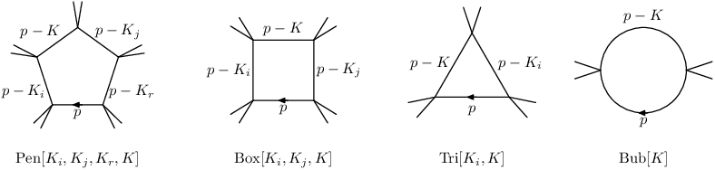
Now we list our results (Figure 1 shows the graphs that correspond to various formulas):

•

(a) Pentagon: It is given by

\displaystyle\textrm{Pen}[K_{i},K_{j},K_{r},K]

\displaystyle=

\displaystyle{\cal T}^{(N)}(\widetilde{\ell}_{(i,j,r)})\cdot D_{i}(\widetilde{\ell}_{(i,j,r)})D_{j}(\widetilde{\ell}_{(i,j,r)})D_{r}(\widetilde{\ell}_{(i,j,r)}).\quad

(11)

where $\widetilde{\ell}_{(i,j,r)}$ is given by (109) and $D_{i}(\widetilde{\ell})$ is given by (39).

•

(b) Box: It is given by

	$\displaystyle\mathrm{Box}[K_{i},K_{j},K]$	$\displaystyle=$	$\displaystyle\frac{1}{2}\left({\cal T}^{(N)}(\widetilde{\ell}_{ij})\cdot D_{i}(\widetilde{\ell}_{ij})D_{j}(\widetilde{\ell}_{ij})-\sum_{r\neq i,j}{\textrm{Pen}[K_{i},K_{j},K_{r},K]\over D_{r}(\widetilde{\ell}_{ij})}\right)\Bigg\|{\begin{matrix}\\ \left\{\scriptsize\begin{matrix}\left\|\ell\right]&\rightarrow&\left\|P_{ji,2}\right]\\ \left\|\ell\right\rangle&\rightarrow&\left\|P_{ji,1}\right\rangle\end{matrix}\right.\end{matrix}}$		(12)
			$\displaystyle+\{P_{ji,1}\leftrightarrow P_{ji,2}\}\quad$		(12)

where $\widetilde{\ell}_{ij}$ are given by (116) or (214), while $\left|P_{ji,a}\right\rangle$ and $\left|P_{ji,a}\right]$ are given by (184).

•

	$\displaystyle\textrm{Tri}[K_{s},K]$	$\displaystyle=$	$\displaystyle\frac{1}{2}\frac{(K^{2})^{N+1}}{(-{\beta}\sqrt{1-u})^{N+1}(\sqrt{-4q_{s}^{2}K^{2}})^{N+1}}\frac{1}{(N+1)!\left\langle P_{s,1}~P_{s,2}\right\rangle^{N+1}}$		(13)
			$\displaystyle\frac{d^{N+1}}{d\tau^{N+1}}\left({\left\langle\ell\|K\|\ell\right]^{N+1}\over(K^{2})^{N+1}}{\cal T}^{(N)}(\widetilde{\ell})\cdot D_{s}(\widetilde{\ell})\Bigg\|{\scriptsize\begin{matrix}\\ \left\{\begin{matrix}\left\|\ell\right]&\rightarrow&\|Q_{s}(u)\left\|\ell\right\rangle\hskip 8.19447pt\hskip 8.19447pt\\ \left\|\ell\right\rangle&\rightarrow&\left\|P_{s,1}-\tau P_{s,2}\right\rangle\end{matrix}\right.\end{matrix}}+\{P_{s,1}\leftrightarrow P_{s,2}\}\right)\Big\|_{\tau\to 0}\qquad$		(13)

where $\widetilde{\ell}$ is given by (10), $Q_{s}(u)$ is given by (173), and $P_{s,a}$ is given by (185).

It is worth to emphasize the ordering of replacement. We need to replace $\left|\ell\right]\rightarrow|Q_{s}(u)\left|\ell\right\rangle$ first where $\left|\ell\right\rangle$ shows up. Then we replace $\left|\ell\right\rangle\rightarrow\left|P_{s,1}-\tau P_{s,2}\right\rangle$ . To denote this ordering, we have put the first replacement above the second one. Similar understanding should apply for later formulas.

Refer to caption — Figure 1: The figures corresponding to various formulas are shown. Notice the order of the propagators can be changed. Our convention is that all external momenta are taken outgoing.

•

(d) Bubble:The bubble coefficient is⁵⁵ 5 Here we give the formula with general choice of auxiliary null momentum $\eta$ . For some special choice, the formula may be modified, which can be found at the end of Section 4.

\displaystyle\textrm{Bub}[K]

\displaystyle=

\displaystyle(K^{2})^{N+1}\sum_{q=0}^{N}{(-1)^{q}\over q!}{d^{q}\over ds^{q}}\left({\cal B}_{N,N-q}^{(0)}(s)+\sum_{r=1}^{k}\sum_{a=q}^{N}\left[{\cal B}_{N,N-a}^{(r,a-q,1)}(s)-{\cal B}_{N,N-a}^{(r,a-q,2)}(s)\right]\right)\Bigg|_{s\rightarrow 0}\qquad

(14)

\displaystyle{\cal B}_{N,t}^{(0)}(s)

\displaystyle=

\displaystyle{d^{N}\over d\tau^{N}}\left[{(2\eta\cdot K)^{t+1}\over(t+1)(K^{2})^{t+1}}{1\over N![\eta|\widetilde{\eta}K|\eta]^{N}\left\langle\ell~\eta\right\rangle^{N+1}}\left(\frac{\left\langle\ell|K|\ell\right]^{N}}{(K^{2})^{N}}{\cal T}^{(N)}(\widetilde{\ell})\right)\Bigg|{\scriptsize\begin{matrix}\\ \left\{\begin{matrix}\left|\ell\right]&\rightarrow&|K+s\eta\left|\ell\right\rangle\\ \left|\ell\right\rangle&\rightarrow&|K-\tau\widetilde{\eta}|\eta]\end{matrix}\right.\end{matrix}}\right]\Bigg|_{\tau\rightarrow 0}

(15)

	$\displaystyle{\cal B}_{N,t}^{(r,b,1)}(s)$	$\displaystyle=$	$\displaystyle{1\over b!~({\beta}\sqrt{1-u})^{b+1}~(\sqrt{-4q_{r}^{2}K^{2}})^{b+1}\left\langle P_{r,1}~P_{r,2}\right\rangle^{b}}{d^{b}\over d\tau^{b}}\left[{1\over t+1}{\left\langle\ell\|\eta\|P_{r,1}\right]^{t+1}\over\left\langle\ell\|K\|P_{r,1}\right]^{t+1}}{\left\langle\ell\|Q_{r}(u)\eta\|\ell\right\rangle^{b}\over\left\langle\ell\|\eta K\|\ell\right\rangle^{N+1}}\right.\qquad$		(16)
			$\displaystyle\left.\times\left(\frac{\left\langle\ell\|K\|\ell\right]^{N+1}}{(K^{2})^{N+1}}{\cal T}^{(N)}(\widetilde{\ell})\cdot D_{r}(\widetilde{\ell})\right)\Bigg\|{\scriptsize\begin{matrix}\\ \left\{\begin{matrix}\left\|\ell\right]&\rightarrow&\|K+s\eta\left\|\ell\right\rangle~~~\\ \left\|\ell\right\rangle&\rightarrow&\left\|P_{r,1}-\tau P_{r,2}\right\rangle\end{matrix}\right.\end{matrix}}\right]\Bigg\|_{\tau\rightarrow 0}\qquad$		(16)

	$\displaystyle{\cal B}_{N,t}^{(r,b,2)}(s)$	$\displaystyle=$	$\displaystyle{1\over b!~({\beta}\sqrt{1-u})^{b+1}~(\sqrt{-4q_{r}^{2}K^{2}})^{b+1}\left\langle P_{r,1}~P_{r,2}\right\rangle^{b}}{d^{b}\over d\tau^{b}}\left[{1\over t+1}{\left\langle\ell\|\eta\|P_{r,2}\right]^{t+1}\over\left\langle\ell\|K\|P_{r,2}\right]^{t+1}}{\left\langle\ell\|Q_{r}(u)\eta\|\ell\right\rangle^{b}\over\left\langle\ell\|\eta K\|\ell\right\rangle^{N+1}}\right.\qquad$		(17)
			$\displaystyle\left.\times\left(\frac{\left\langle\ell\|K\|\ell\right]^{N+1}}{(K^{2})^{N+1}}{\cal T}^{(N)}(\widetilde{\ell})\cdot D_{r}(\widetilde{\ell})\right)\Bigg\|{\scriptsize\begin{matrix}\\ \left\{\begin{matrix}\left\|\ell\right]&\rightarrow&\|K+s\eta\left\|\ell\right\rangle~~~\\ \left\|\ell\right\rangle&\rightarrow&\left\|P_{r,2}-\tau P_{r,1}\right\rangle\end{matrix}\right.\end{matrix}}\right]\Bigg\|_{\tau\rightarrow 0}\qquad$		(17)

where $\widetilde{\ell}$ is given by (10), $Q_{r}(u)$ is given by (173), $P_{r,a}$ is given by (186), and $\eta,\widetilde{\eta}$ are arbitrary, generically chosen null vectors. The summation over $r$ includes all the $D_{r}(\widetilde{\ell})$ that appear in the denominator of ${\cal T}(\widetilde{\ell})$ .

If $N\leq-2$ , there are contributions only from boxes and pentagons. If $N\geq-1$ , contributions from triangles will kick in, and finally if $N\geq 0$ , bubble contributions show up as well. Similar observation has been made in [5].

Our formula should be suitable for both analytic and numerical calculations. For numerical calculation, since our result should be polynomial of $u$ , so we should have a way to get coefficients of $u^{a}$ numerically. This can be done by using discrete Fourier transformation method[35].

2 D-dimensional unitarity method

In this section, we briefly review the $D$ -dimensional unitarity method [45] and define various forms of tree level input. In the process, we also establish our conventions and give definitions of some variables and functions. Some preliminary knowledge about spinor formalism [53] and color decompositions [54] can be found in two classic reviews [55, 56]. Here we only emphasize that, we use the “twistor” convention for the square bracket $[i~j]$ , so that $2k_{i}\cdot k_{j}=\left\langle i~j\right\rangle[i~j]$ .

Let’s start with the following expression for a double-cut ( $K^{2}$ -channel) integral:

\displaystyle C[{\cal A}]\big|_{K^{2}-\textrm{channel}}

\displaystyle=

\displaystyle-i(4\pi)^{D/2}\int{d^{D}p\over(2\pi)^{D}}~\delta(p^{2}-M_{1}^{2})~\delta((p-K)^{2}-M_{2}^{2})~{\cal T}(p).\quad

(18)

Compared with the full amplitude expressed in (4), i.e.

\displaystyle{\cal A}=\sum_{n,i}~c_{n,i}(\mu^{2})\otimes I_{n}^{D,(i)}[1],\quad

(19)

the cut integral (18) can be understood as

\displaystyle C[{\cal A}]\big|_{K^{2}-\textrm{channel}}=\sum_{n,i}~c_{n,i}(\mu^{2})\otimes C[I_{n}^{D,(i)}[1]]\big|_{K^{2}-\textrm{channel}},\quad

(20)

where the cut master integral is

\displaystyle C\left[I_{n}^{D}[1]\right]\big|_{K^{2}-\textrm{channel}}=-i(4\pi)^{D/2}\int{d^{D}p\over(2\pi)^{D}}~{\delta(p^{2}-M_{1}^{2})~\delta((p-K)^{2}-M_{2}^{2})\over\prod_{i=1}^{n-2}((p-K_{i})^{2}-m_{i}^{2})}.\quad

(21)

Those master integral, which don’t contain two propagators that correspond to the two $\delta$ -functions, will not appear in the cut integral (20). By evaluating different cut integrals, we can get all coefficients $c_{n,i}(\mu^{2})$ .

In next subsection, we will briefly review how to simplify double cut phase-space integration. This technique is the foundation of our method. After these transformations, we can describe the structure of cut integrands, from which it is possible to read off coefficients directly.

2.1 Simplify phase-space integral

The internal loop momentum $p$ is $(D=4-2\epsilon)$ -dimensional and can be decomposed as

\displaystyle p=\widetilde{\ell}+\vec{\mu};\qquad\int d^{4-2\epsilon}p=\int d^{-2\epsilon}\mu\int d^{4}\widetilde{\ell}\ ,\quad

(22)

where $\widetilde{\ell}$ is 4-dimensional and $\vec{\mu}$ is $(-2\epsilon)$ -dimensional. We can further decompose $\widetilde{\ell}$ as

\displaystyle\widetilde{\ell}=\ell+zK,\qquad\ell^{2}=0;\qquad\int d^{4}\widetilde{\ell}=\int dz~d^{4}\ell~\delta^{(+)}(\ell^{2})~(2\ell\cdot K),\qquad

(23)

where $K$ is the momentum across the cut. $\ell$ is a massless 4-momentum, and can be expressed with spinor variables as [57]

\displaystyle\ell=tP_{\lambda\widetilde{\lambda}},\qquad P_{\lambda\widetilde{\lambda}}=\lambda\widetilde{\lambda}=\left|\ell\right\rangle\left|\ell\right];\qquad\int d^{4}\ell\ \delta^{(+)}(\ell^{2})

\displaystyle=

\displaystyle\int\left\langle\ell~d\ell\right\rangle[\ell~d\ell]\int t~dt.

(24)

The corresponding measure has also been given.

The Lorentz-invariant phase-space (LIPS) of a double cut is defined by inserting two $\delta$ -functions representing the cut conditions:

$\displaystyle\int d^{4-2\epsilon}\Phi$	$\displaystyle\equiv$	$\displaystyle\int{d^{4-2\epsilon}p}~\delta(p^{2}-M_{1}^{2})\delta((p-K)^{2}-M_{2}^{2})$	(25)
	$\displaystyle=$	$\displaystyle\frac{(4\pi)^{\epsilon}}{\Gamma(-\epsilon)}~\int d\mu^{2}~(\mu^{2})^{-1-\epsilon}\int{d^{4}\widetilde{\ell}}~\delta(\widetilde{\ell}^{2}-\mu^{2}-M_{1}^{2})~\delta((\widetilde{\ell}-K)^{2}-\mu^{2}-M_{2}^{2})$
	$\displaystyle=$	$\displaystyle\frac{(4\pi)^{\epsilon}}{\Gamma(-\epsilon)}~\int d\mu^{2}~(\mu^{2})^{-1-\epsilon}\int dz~d^{4}\ell~\delta^{(+)}(\ell^{2})~(2\ell\cdot K)$
		$\displaystyle\qquad\times\delta(z(1-z)K^{2}+z(M_{1}^{2}-M_{2}^{2})-M_{1}^{2}-\mu^{2})~\delta(-2\ell\cdot K+(1-2z)K^{2}+M_{1}^{2}-M_{2}^{2}).$

We can firstly perform the integral over $z$ with $\delta$ -function $\delta(z(1-z)K^{2}+z(M_{1}^{2}-M_{2}^{2})-M_{1}^{2}-\mu^{2})$ to reach

	$\displaystyle\int d^{4-2\epsilon}\Phi$	$\displaystyle=$	$\displaystyle\frac{(4\pi)^{\epsilon}}{\Gamma(-\epsilon)}~\int d\mu^{2}~(\mu^{2})^{-1-\epsilon}\int d^{4}\ell~\delta^{(+)}(\ell^{2})~\delta(-2\ell\cdot K+(1-2z)K^{2}+M_{1}^{2}-M_{2}^{2})$		(26)
		$\displaystyle=$	$\displaystyle\frac{(4\pi)^{\epsilon}}{\Gamma(-\epsilon)}~\int d\mu^{2}~(\mu^{2})^{-1-\epsilon}\int\left\langle\ell~d\ell\right\rangle[\ell~d\ell]\int t~dt~\delta(-2tK\cdot P_{\lambda\widetilde{\lambda}}+(1-2z)K^{2}+M_{1}^{2}-M_{2}^{2}),$		(26)

where $z$ is fixed by solving the $\delta$ -function as

\displaystyle z={(K^{2}+M_{1}^{2}-M_{2}^{2})-\sqrt{\Delta[K,M_{1},M_{2}]-4K^{2}\mu^{2}}\over 2K^{2}}~,\qquad

(27)

with

\displaystyle\Delta[K,M_{1},M_{2}]\equiv(K^{2})^{2}+(M_{1}^{2})^{2}+(M_{2}^{2})^{2}-2K^{2}M_{1}^{2}-2K^{2}M_{2}^{2}-2M_{1}^{2}M_{2}^{2}\ .\quad

(28)

Then we can perform the integral over $t$ with the remaining $\delta$ -function to reach

\displaystyle\int d^{4-2\epsilon}\Phi

\displaystyle=

\displaystyle\frac{(4\pi)^{\epsilon}}{\Gamma(-\epsilon)}~\int d\mu^{2}~(\mu^{2})^{-1-\epsilon}\int\left\langle\ell~d\ell\right\rangle[\ell~d\ell]{(1-2z)K^{2}+M_{1}^{2}-M_{2}^{2}\over(2K\cdot P_{\lambda\widetilde{\lambda}})^{2}}~,\quad

(29)

and $t$ is

\displaystyle t={(1-2z)K^{2}+M_{1}^{2}-M_{2}^{2}\over 2K\cdot P_{\lambda\widetilde{\lambda}}}.\quad

(30)

For convenience, one can redefine the $\mu^{2}$ -integral measure as

\displaystyle\int d\mu^{2}(\mu^{2})^{-1-\epsilon}=\left({\Delta[K,M_{1},M_{2}]\over 4K^{2}}\right)^{-\epsilon}\int_{0}^{1}du\ u^{-1-\epsilon},

where the relation between $u$ and $\mu^{2}$ is given by

\displaystyle u\equiv{4K^{2}\mu^{2}\over\Delta[K,M_{1},M_{2}]}.\quad

(31)

Then we can rewrite $z,t$ as

\displaystyle z={{\alpha}-{\beta}\sqrt{1-u}\over 2},\qquad t={{\beta}\sqrt{1-u}~{K^{2}\over 2K\cdot P_{\lambda\widetilde{\lambda}}}},\quad

(32)

where

\displaystyle{\alpha}={K^{2}+M_{1}^{2}-M_{2}^{2}\over K^{2}},\qquad{\beta}={\sqrt{\Delta[K,M_{1},M_{2}]}\over K^{2}}.\quad

(33)

Notice that when $M_{1}=M_{2}=0$ we have ${\alpha}={\beta}=1$ , thus reproducing the massless case. A useful relation between $z$ and $u$ is the following:

\displaystyle(1-2z)+{M_{1}^{2}-M_{2}^{2}\over K^{2}}={\beta}\sqrt{1-u}.\quad

(34)

After these evaluations, the cut integral (18) is transformed to

	$\displaystyle C[{\cal A}]$	$\displaystyle=$	$\displaystyle\frac{(4\pi)^{\epsilon}}{i\pi^{D/2}\Gamma(-\epsilon)}~\int d\mu^{2}~(\mu^{2})^{-1-\epsilon}\int\left\langle\ell~d\ell\right\rangle[\ell~d\ell]{(1-2z)K^{2}+M_{1}^{2}-M_{2}^{2}\over(2K\cdot P_{\lambda\widetilde{\lambda}})^{2}}{\cal T}(p)\quad$		(35)
		$\displaystyle=$	$\displaystyle\frac{(4\pi)^{\epsilon}}{i\pi^{D/2}\Gamma(-\epsilon)}~\left({\Delta[K,M_{1},M_{2}]\over 4K^{2}}\right)^{-\epsilon}\int_{0}^{1}du\ u^{-1-\epsilon}\int\left\langle\ell~d\ell\right\rangle[\ell~d\ell]~{\beta}\sqrt{1-u}~{K^{2}\over(2K\cdot P_{\lambda\widetilde{\lambda}})^{2}}{\cal T}(p).\qquad$		(35)

Here ${\cal T}(p)$ should be interpreted as

\displaystyle{\cal T}(p)={\cal T}(\widetilde{\ell}~,\mu^{2})={\cal T}(tP_{\lambda\widetilde{\lambda}}+zK~,\mu^{2})={\cal T}(\left|\ell\right\rangle,\left|\ell\right],\mu^{2}),\quad

(36)

with $z$ and $t$ defined as in (32). In the following, we may write ${\cal T}(p)$ as ${\cal T}(\widetilde{\ell})$ where the dependence on $\mu^{2}$ is implicitly included, with $\widetilde{\ell}$ being interpreted as

\displaystyle\widetilde{\ell}=tP_{\lambda\widetilde{\lambda}}+zK={K^{2}\over\left\langle\ell|K|\ell\right]}\left[-{\beta}\sqrt{1-u}\left(P_{\lambda\widetilde{\lambda}}-{K\cdot P_{\lambda\widetilde{\lambda}}\over K^{2}}K\right)-{\alpha}{K\cdot P_{\lambda\widetilde{\lambda}}\over K^{2}}K\right].\quad

(37)

2.2 Standard form of the input

For a double cut of physical amplitudes, it is always possible (for example from Feynman rule) to write ${\cal T}(p)$ as a sum of terms of the following form

\displaystyle{\cal T}^{(n)}_{sf}(\widetilde{\ell})=\frac{\prod_{j=1}^{n+k}(-2\widetilde{\ell}\cdot P_{j})}{\prod_{i=1}^{k}D_{i}(\widetilde{\ell})},\quad

(38)

where $D_{i}(\widetilde{\ell})$ is the propagator

\displaystyle D_{i}(\widetilde{\ell})\equiv(\widetilde{\ell}-K_{i})^{2}-\mu^{2}-m_{i}^{2}=-2\widetilde{\ell}\cdot K_{i}+K_{i}^{2}+M_{1}^{2}-m_{i}^{2}.\quad~~~~~

(39)

We emphasize that the relation $\widetilde{\ell}^{2}=M_{1}^{2}+\mu^{2}$ from the cut constraint is always assumed in the input.

We will call the form of ${\cal T}(p)$ like (38) as the standard form, where there are only $D_{i}(\widetilde{\ell})$ in the denominator. We will frequently use an important quantity – the degree for $p$ (or equivalently for $\widetilde{\ell}$ ). The degree of ${\cal T}(p)$ is defined as the degree of numerator minus the degree of denominator. For the standard form (81), the degree is $n$ , which was shown explicitly in the superscript.

After simplifying the phase-space integration, the cut integral for the standard form can be written in the form of (35):

\displaystyle\frac{(4\pi)^{\epsilon}}{i\pi^{D/2}\Gamma(-\epsilon)}~\left({\Delta[K,M_{1},M_{2}]\over 4K^{2}}\right)^{-\epsilon}\int_{0}^{1}du\ u^{-1-\epsilon}\int\left\langle\ell~d\ell\right\rangle[\ell~d\ell]~{\beta}\sqrt{1-u}~{(K^{2})^{n+1}\over\left\langle\ell|K|\ell\right]^{n+2}}{\prod_{j=1}^{n+k}\left\langle\ell|R_{j}|\ell\right]\over\prod_{i=1}^{k}\left\langle\ell|Q_{i}|\ell\right]}~,\qquad

(40)

where

	$\displaystyle R_{j}(u)$	$\displaystyle\equiv$	$\displaystyle-{\beta}(\sqrt{1-u})\left(P_{j}-{P_{j}\cdot K\over K^{2}}K\right)-{\alpha}{(P_{j}\cdot K)\over K^{2}}K,$
	$\displaystyle Q_{i}(u)$	$\displaystyle\equiv$	$\displaystyle-{\beta}(\sqrt{1-u})\left(K_{i}-{K_{i}\cdot K\over K^{2}}K\right)-\left({\alpha}{(K_{i}\cdot K)\over K^{2}}-{K_{i}^{2}+M_{1}^{2}-m_{i}^{2}\over K^{2}}\right)K,\quad$

and ${\alpha},{\beta}$ are given by (33). We should notice the equivalent relations at the integrand level as

\displaystyle-2\widetilde{\ell}\cdot P_{j}

\displaystyle=

\displaystyle{K^{2}\over\left\langle\ell|K|\ell\right]}\left\langle\ell|R_{j}|\ell\right],\qquad D_{i}(\widetilde{\ell})={K^{2}\over\left\langle\ell|K|\ell\right]}\left\langle\ell|Q_{i}|\ell\right],\quad

(41)

and therefore

\displaystyle{\cal T}^{(n)}_{sf}(\widetilde{\ell})

\displaystyle=

\displaystyle{(K^{2})^{n}\over\left\langle\ell|K|\ell\right]^{n}}{\prod_{j=1}^{n+k}\left\langle\ell|R_{j}|\ell\right]\over\prod_{i=1}^{k}\left\langle\ell|Q_{i}|\ell\right]}.\quad

(42)

For the cut integral with standard form input (40), we can read off coefficients directly by using several formulas, which are reviewed in the Appendix A.

2.3 General form of tree level input and spurious pole

We now consider the general form of inputs. In unitarity method, the input needed is a collection of (on-shell) tree level amplitudes. By using the on-shell recursion relations, very compact expressions for the tree level input can be obtained. However, such compact expressions usually contain some spurious poles.

A general form of ${\cal T}(p)$ that with a spurious pole can be written as (for simplicity, we only consider the case of single spurious pole, multi-spurious pole is a trivial generalization)

\displaystyle{\cal T}_{sp}^{(N)}(\widetilde{\ell})=\sum_{t}c_{t}\frac{\prod_{j=1}^{n_{t}+k_{t}+d}(-2\widetilde{\ell}\cdot P_{j})}{S_{d}\prod_{i=1}^{k_{t}}D_{i}(\widetilde{\ell})},\quad

(43)

where $c_{t}$ are coefficients that do not depend on $\widetilde{\ell}$ , but may depend on $\mu^{2}$ . $S_{d}$ is the spurious pole with degree $d$ and can be generally expressed as

	$\displaystyle S_{d}$	$\displaystyle=$	$\displaystyle s_{0}+\sum_{i}s_{i}(-2\widetilde{\ell}\cdot V_{1,i})+\sum_{i_{1},i_{2}}s_{i_{1},i_{2}}(-2\widetilde{\ell}\cdot V_{2,i_{1}})(-2\widetilde{\ell}\cdot V_{2,i_{2}})+...\quad$		(44)
			$\displaystyle+\sum_{i_{1},\dots,i_{d}}s_{i_{1},...,i_{d}}(-2\widetilde{\ell}\cdot V_{d,i_{1}})(-2\widetilde{\ell}\cdot V_{d,i_{2}})...(-2\widetilde{\ell}\cdot V_{d,i_{d}}).$		(44)

The degree of ${\cal T}_{sp}^{(N)}(\widetilde{\ell})$ is $N$ , which is defined as the maximum of $n_{t}$

\displaystyle N=\textrm{Max}\{n_{t}\}.

(45)

After putting into (40), ${\cal T}_{sp}^{(N)}(\widetilde{\ell})$ can be rewritten by using the relation (41) as:

\displaystyle{\cal T}_{sp}^{(N)}(\widetilde{\ell})=\sum_{t}c_{t}{(K^{2})^{n_{t}}\over\left\langle\ell|K|\ell\right]^{n_{t}}}{\prod_{j=1}^{n_{t}+k_{t}+d}\left\langle\ell|R_{j}|\ell\right]\over{\widehat{S}}_{d}\prod_{i=1}^{k_{t}}\left\langle\ell|Q_{i}|\ell\right]},\qquad

(46)

where

	$\displaystyle{\widehat{S}}_{d}$	$\displaystyle=$	$\displaystyle s_{0}{\left\langle\ell\|K\|\ell\right]^{d}\over(K^{2})^{d}}+\sum_{i}{\left\langle\ell\|K\|\ell\right]^{d-1}\over(K^{2})^{d-1}}s_{i}\left\langle\ell\|\widetilde{V}_{1,i}\|\ell\right]+\sum_{i_{1},i_{2}}{\left\langle\ell\|K\|\ell\right]^{d-2}\over(K^{2})^{d-2}}s_{i_{1},i_{2}}\left\langle\ell\|\widetilde{V}_{2,i_{1}}\|\ell\right]\left\langle\ell\|\widetilde{V}_{2,i_{2}}\|\ell\right]+...\quad$		(47)
			$\displaystyle+\sum_{i_{1},...,i_{d}}s_{i_{1},...,i_{d}}\left\langle\ell\|\widetilde{V}_{d,i_{1}}\|\ell\right]\left\langle\ell\|\widetilde{V}_{d,i_{2}}\|\ell\right]...\left\langle\ell\|\widetilde{V}_{d,i_{d}}\|\ell\right],$		(47)

and $\widetilde{V}_{t,i_{z}}$ is obtained from $V_{t,i_{z}}$ just as that $R_{j}$ obtained from $P_{j}$ .

For a physical amplitude, poles other than $D_{i}(\widetilde{\ell})$ are all spurious. It is always possible to regroup terms into an expression free of spurious poles, i.e. a sum of standard forms:

\displaystyle{\cal T}_{nsp}^{(N)}(\widetilde{\ell})=\sum_{r}b_{r}\frac{\prod_{j=1}^{n_{r}+k_{r}}(-2\widetilde{\ell}\cdot P_{j})}{\prod_{i=1}^{k_{r}}D_{i}(\widetilde{\ell})}=\sum_{r}b_{r}{(K^{2})^{n_{r}}\over\left\langle\ell|K|\ell\right]^{n_{r}}}{\prod_{j=1}^{n_{r}+k_{r}}\left\langle\ell|R_{j}|\ell\right]\over\prod_{i=1}^{k_{r}}\left\langle\ell|Q_{i}|\ell\right]}.\quad

(48)

$b_{r}$ are coefficients that do not depend on $\widetilde{\ell}$ , but may depend on $\mu^{2}$ . The degree, now the maximum of $n_{r}$ , should also be $N$ .

An important observation is that: to go from ${\cal T}_{sp}^{(N)}(\widetilde{\ell})$ to ${\cal T}_{nsp}^{(N)}(\widetilde{\ell})$ , we only need to apply some spinor identities to remove the spurious pole, while $\widetilde{\ell}$ must satisfy the two on-shell conditions:

\displaystyle\widetilde{\ell}^{2}-\mu^{2}-M_{1}^{2}=0,\qquad(\widetilde{\ell}-K)^{2}-\mu^{2}-M_{2}^{2}=0.\quad

(49)

This observation will be important in the proof of the generalization in Section 4.

3 Looking at the formulas

The formulas we have known (collected in Appendix A) are applicable for the standard form ${\cal T}_{sf}(p)$ , in which the key requirement is that there is no spurious pole, i.e. only propagators $D(\widetilde{\ell})$ appear in the denominator. One may expect to remove the spurious pole in a general input to reach the standard form, since it’s possible in principle. However, in general practice, this procedure is very complicated and we do not have well-defined algorithm to do that. Besides, the most compact expression of the tree level input usually has spurious poles. After removing the spurious poles, the expression may expand quite a lot, which leads the computation to be less efficient. Therefore, it is important to be able to generalize formulas to the case with spurious pole, while keeping the compactness of the tree input.

In the following, we will study the previous known formulas for the standard forms input from a new point of view, by which we can gain some insights on how to generalize the formulas to the case with spurious poles.

3.1 Splitting of the integrand

We start from the integrand in (40)

\displaystyle I

\displaystyle=

\displaystyle{(K^{2})^{n+1}\over\left\langle\ell|K|\ell\right]^{n+2}}{\prod_{j=1}^{k+n}\left\langle\ell|R_{j}|\ell\right]\over\prod_{i=1}^{k}\left\langle\ell|Q_{i}|\ell\right]}~.\qquad\qquad

(50)

Then we do the splitting to reach [46]

\displaystyle I

\displaystyle=

\displaystyle\sum_{i=1}^{k}F_{i}(\lambda){1\over\left\langle\ell|K|\ell\right]\left\langle\ell|Q_{i}|\ell\right]}+\sum_{j=0}^{n}G_{j}(\lambda,\widetilde{\lambda}){1\over\left\langle\ell|K|\ell\right]^{2+j}}~,\qquad

(51)

where

\displaystyle F_{i}(\lambda)={(K^{2})^{n+1}\over\left\langle\ell|KQ_{i}|\ell\right\rangle^{n+1}}{\prod_{j=1}^{k+n}\left\langle\ell|R_{j}Q_{i}|\ell\right\rangle\over\prod_{t=1,t\neq i}^{k}\left\langle\ell|Q_{t}Q_{i}|\ell\right\rangle}~,\qquad

(52)

\displaystyle\sum_{j=0}^{n}G_{j}(\lambda,\widetilde{\lambda}){1\over\left\langle\ell|K|\ell\right]^{2+j}}=(K^{2})^{n+1}\sum_{q=0}^{n}{(-)^{q}\over q!}{d^{q}B_{n,n-q}(s)\over ds^{q}}\Big|_{s=0}~,\qquad

(53)

with

\displaystyle B_{n,t}(s)\equiv{\left\langle\ell|\eta|\ell\right]^{t}\over\left\langle\ell|K|\ell\right]^{2+t}}{\prod_{j=1}^{n+k}\left\langle\ell|R_{j}(K+s\eta)|\ell\right\rangle\over\left\langle\ell|\eta K|\ell\right\rangle^{n}\prod_{p=1}^{k}\left\langle\ell|Q_{p}(K+s\eta)|\ell\right\rangle}~.\qquad

(54)

The box and triangle contributions will come from the $F_{i}$ term in (51), while the $G_{j}$ term will contribute to bubble. Taking the integrand into the cut integral, and extracting the residues of various poles, we can get the final coefficients. With the above splitting, we will know all coefficients by putting them into following expressions:

\displaystyle C[Q_{i},Q_{j},K]

\displaystyle=

\displaystyle{(K^{2})^{n+2}\over 2}\left({\prod_{s=1}^{k+n}\left\langle P_{ji,1}|R_{s}|P_{ji,2}\right]\over\left\langle P_{ji,1}|K|P_{ji,2}\right]^{n+2}\prod_{t=1,t\neq i,j}^{k}\left\langle P_{ji,1}|Q_{t}|P_{ji,2}\right]}+\{P_{ji,1}\leftrightarrow P_{ji,2}\}\right),~~

(55)

for boxes defined by $Q_{i},Q_{j},K$ ,

	$\displaystyle C[Q_{s},K]$	$\displaystyle=$	$\displaystyle{(K^{2})^{n+1}\over 2(\sqrt{\Delta_{s}})^{n+1}}\frac{1}{(n+1)!\left\langle P_{s,1}~P_{s,2}\right\rangle^{n+1}}$		(56)
			$\displaystyle\frac{d^{n+1}}{d\tau^{n+1}}\left({\prod_{j=1}^{k+n}\left\langle P_{s,1}-\tau P_{s,2}\|R_{j}Q_{s}\|P_{s,1}-\tau P_{s,2}\right\rangle\over\prod_{t=1,t\neq s}^{k}\left\langle P_{s,1}-\tau P_{s,2}\|Q_{t}Q_{s}\|P_{s,1}-\tau P_{s,2}\right\rangle}+\{P_{s,1}\leftrightarrow P_{s,2}\}\right)\Bigg\|_{\tau\to 0},\qquad$		(56)

for triangles defined by $Q_{s},K$ and finally for bubble

\displaystyle C[K]=(K^{2})^{n+1}\sum_{q=0}^{n}{(-1)^{q}\over q!}{d^{q}\over ds^{q}}\left.\left({\cal B}_{n,n-q}^{(0)}(s)+\sum_{r=1}^{k}\sum_{a=q}^{n}\left({\cal B}_{n,n-a}^{(r;a-q;1)}(s)-{\cal B}_{n,n-a}^{(r;a-q;2)}(s)\right)\right)\right|_{s=0},~~~~~

(57)

where definition of various variables and functions can be found in Appendix A. The key observation is that all coefficients are just the sum or difference of relative residues of pole. In $F_{i}(\lambda)$ , the poles from $\left\langle\ell|Q_{t}Q_{i}|\ell\right\rangle$ contribute to box, and those from $\left\langle\ell|KQ_{i}|\ell\right\rangle$ contribute to triangle. Bubbles are from the poles in $G_{j}$ , or more precisely, ${\cal B}_{n,t}^{(0)}(s)$ is from the poles $\left\langle\ell|\eta K|\ell\right\rangle$ , and ${\cal B}_{n,t}^{(r,b,1)}(s),{\cal B}_{n,t}^{(r,b,2)}(s)$ are from the poles $\left\langle\ell|Q_{p}(K+s\eta)|\ell\right\rangle$ . Details of the derivations can be found in [46, 47]

Let us recall how do we get above formulas. Starting from standard input, we algebraically simplify it by using splitting technique. Then we perform phase space integrations carefully and add all contributions from physical poles together. If now the input has spurious poles, the same method tells us that we need to perform phase space integration with spurious poles. However, we can not do that in general. The reason is following: (1) The form of spurious poles can be arbitrary and we do not know how to write them down; (2) To perform the phase space integration, we need to write it into total derivative and then take residues. For a given spurious pole, we do not know how to perform both manipulations.

Because these reasons, it seems impossible to find results by standard method. However, considering these poles are all spurious, this means that even we are able to extract the residues of spurious poles term by term, their sum should vanish from physical point of view. In this sense, we can expect that the formulas can be generalized to the general form without many modifications. Then the question is how to do it? Which new method will enable us to do it?

To be able to proceed, we find that we need to take a new perspective in understanding above results. Remembering that when the spurious poles show up, there are at least two terms with spurious pole, so the added result will cancel out. In another word, we will have following equations (we assume there is only one term of standard form for simplicity):

$\displaystyle{\cal T}(p)$	$\displaystyle\equiv$	$\displaystyle{\prod_{j=1}^{n+k}(-2\widetilde{\ell}\cdot P_{j})\over\prod_{i=1}^{k}D_{i}(\widetilde{\ell})}\qquad$	(58)
	$\displaystyle=$	$\displaystyle\sum_{t,\{i_{t}\}}{s_{i_{1},i_{2},...,i_{t}}(-2\widetilde{\ell}\cdot V_{t,i_{1}})(-2\widetilde{\ell}\cdot V_{t,i_{2}})...(-2\widetilde{\ell}\cdot V_{t,i_{t}})\prod_{j=1}^{n+k}(-2\widetilde{\ell}\cdot P_{j})\over S_{d}\prod_{i=1}^{k}D_{i}(\widetilde{\ell})}\qquad$	(59)
	$\displaystyle=$	$\displaystyle\sum_{t}c_{t}{\prod_{j=1}^{n_{t}+k_{t}}(-2\widetilde{\ell}\cdot P_{j})\over S_{d}\prod_{i=1}^{k_{t}}D_{i}(\widetilde{\ell})}\qquad$	(60)

where $S_{d}$ is given in (44)and $\{i_{t}\}$ means the set $\{i_{1},...,i_{t}\}$ . Among these three forms, the first form is the one without the spurious pole, while the third form is the one obtained by using on-shell tree level recursion relation. The second one is the bridge bring the first one to the third one.

After putting into (40), we have following three forms for the integrand

$\displaystyle I[\left\|\ell\right\rangle,\left\|\ell\right]]$	$\displaystyle\equiv$	$\displaystyle{(K^{2})^{n+1}\over\left\langle\ell\|K\|\ell\right]^{n+2}}{\prod_{j=1}^{n+k}\left\langle\ell\|R_{j}\|\ell\right]\over\prod_{i=1}^{k}\left\langle\ell\|Q_{i}\|\ell\right]}\qquad$	(61)
	$\displaystyle=$	$\displaystyle\sum_{t,\{i_{t}\}}s_{i_{1},i_{2},...,i_{t}}{(K^{2})^{n+1+t-d}\over\left\langle\ell\|K\|\ell\right]^{n+2+t-d}}{\prod_{z=1}^{t}\left\langle\ell\|\widetilde{V}_{t,i_{z}}\|\ell\right]\prod_{j=1}^{n+k}\left\langle\ell\|R_{j}\|\ell\right]\over\widehat{S}_{d}[\left\|\ell\right\rangle,\|\ell]]\prod_{i=1}^{k}\left\langle\ell\|Q_{i}\|\ell\right]}\qquad$	(62)
	$\displaystyle=$	$\displaystyle\sum_{t}c_{t}{(K^{2})^{n_{t}+1-d}\over\left\langle\ell\|K\|\ell\right]^{n_{t}+2-d}}{\prod_{j=1}^{n_{t}+k_{t}}\left\langle\ell\|R_{j}\|\ell\right]\over\widehat{S}_{d}[\left\|\ell\right\rangle,\|\ell]]\prod_{i=1}^{k_{t}}\left\langle\ell\|Q_{i}\|\ell\right]}\qquad$	(63)

which should be considered as function of $\left|\ell\right\rangle$ and $\left|\ell\right]$ . It is important that we have treated $\left|\ell\right\rangle$ and $\left|\ell\right]$ as independent variables.

3.2 The splitting result for box and triangle

The next step is to find the expression contributing to various coefficients.

Let us start from the box and triangle. From the form (50) we can see that the relative expression (i.e., for box and triangle having $Q_{i}$ ) is

\displaystyle F_{i}^{(I)}

\displaystyle=

\displaystyle{(K^{2})^{n+1}\over\left\langle\ell|KQ_{i}|\ell\right\rangle^{n+1}}{\prod_{j=1}^{n+k}\left\langle\ell|R_{j}Q_{i}|\ell\right\rangle\over\prod_{t=1,t\neq i}^{k}\left\langle\ell|Q_{t}Q_{i}|\ell\right\rangle}~.\qquad

(64)

Comparing (64) and (50) we found that it is obtained from (50) by following manipulations:

•

(a) Multiplying $\left\langle\ell|K|\ell\right]$ and $\left\langle\ell|Q_{i}|\ell\right]$ at (50);
•

(b) Then replacing $\left|\ell\right]\to Q_{i}\left|\ell\right\rangle$ .

Using this observation, we can get two results from (62) and (63) as following

\displaystyle F_{i}^{(II)}

\displaystyle=

\displaystyle\sum_{t,\{i_{t}\}}s_{i_{1},i_{2},...,i_{t}}{(K^{2})^{n+1+t-d}\over\left\langle\ell|KQ_{i}|\ell\right\rangle^{n+1+t-d}}{\prod_{z=1}^{t}\left\langle\ell|\widetilde{V}_{t,i_{z}}Q_{i}|\ell\right\rangle\prod_{j=1}^{n+k}\left\langle\ell|R_{j}Q_{i}|\ell\right\rangle\over\widehat{S}_{d}[\left|\ell\right\rangle,Q_{i}\left|\ell\right\rangle]\prod_{\widetilde{i}=1,\widetilde{i}\neq i}^{k}\left\langle\ell|Q_{\widetilde{i}}Q_{i}|\ell\right\rangle}~~~

(65)

and

\displaystyle F_{i}^{(III)}

\displaystyle=

\displaystyle\sum_{t}c_{t}{(K^{2})^{n_{t}+1-d}\over\left\langle\ell|KQ_{i}|\ell\right\rangle^{n_{t}+1-d}}{\prod_{j=1}^{n_{t}+k_{t}}\left\langle\ell|R_{j}Q_{i}|\ell\right\rangle\left\langle\ell|Q_{i}Q_{i}|\ell\right\rangle\over\widehat{S}_{d}[\left|\ell\right\rangle,Q_{i}\left|\ell\right\rangle]\prod_{\widetilde{i}=1}^{k_{t}}\left\langle\ell|Q_{\widetilde{i}}Q_{i}|\ell\right\rangle}~~~

(66)

It is worth to give a remark regarding the expression (66). In this formula we have factor $\left\langle\ell|Q_{i}Q_{i}|\ell\right\rangle=0$ in numerator. If there is same factor $\left\langle\ell|Q_{i}Q_{i}|\ell\right\rangle$ in denominator, then both factors will cancel each other, but if there is no such factor in denominator, we know immediately that this term contributes zero. A subtle point for box formula will be discussed in Section 3.4.

Since three expressions (61), (62) and (63) are equal to each other at the algebraic level. After the same algebraic manipulation, we should have that three expressions (64), (65) and (66) are equal to each other too.

Now we can read out the expression for the box and triangle coefficients.

3.3 Read the coefficients

The coefficients of box from (64) is

	$\displaystyle C[Q_{i},Q_{j},K]^{(I)}$	$\displaystyle=$	$\displaystyle{1\over 2}\left.{(K^{2})^{n+2}\over\left\langle\ell\|KQ_{i}\|\ell\right\rangle^{n+2}}{\prod_{s=1}^{n+k}\left\langle\ell\|R_{s}Q_{i}\|\ell\right\rangle\over\prod_{t=1,t\neq i,j}^{k}\left\langle\ell\|Q_{t}Q_{i}\|\ell\right\rangle}\right\|_{\left\|\ell\right\rangle\to\left\|P_{ji,1}\right\rangle}$		(67)
			$\displaystyle+{1\over 2}\left.{(K^{2})^{n+2}\over\left\langle\ell\|KQ_{i}\|\ell\right\rangle^{n+2}}{\prod_{s=1}^{n+k}\left\langle\ell\|R_{s}Q_{i}\|\ell\right\rangle\over\prod_{t=1,t\neq i,j}^{k}\left\langle\ell\|Q_{t}Q_{i}\|\ell\right\rangle}\right\|_{\left\|\ell\right\rangle\to\left\|P_{ji,2}\right\rangle}~~~$		(67)

which is equivalent to (55) by noticing that

\displaystyle\frac{\left\langle P_{ji,1}|XQ_{i}(u)|P_{ji,1}\right\rangle}{\left\langle P_{ji,1}|X^{\prime}Q_{i}(u)|P_{ji,1}\right\rangle}=\frac{\left\langle P_{ji,1}|X|P_{ji,2}\right]}{\left\langle P_{ji,1}|X^{\prime}|P_{ji,2}\right]}.

(68)

Compared to (64), the coefficient can be obtained by following algebraic actions:

•

(a) Multiplying ${K^{2}\left\langle\ell|Q_{j}Q_{i}|\ell\right\rangle\over 2\left\langle\ell|KQ_{i}|\ell\right\rangle}$ ;
•

(b) Sum up two terms with $\left|\ell\right\rangle\to\left|P_{ji,1}(u)\right\rangle$ and $\left|\ell\right\rangle\to\left|P_{ji,2}(u)\right\rangle$ .

Now it is obviously we should apply same actions to (65) and (66) to get

	$\displaystyle C[Q_{i},Q_{j},K]^{(II)}=\sum_{t,\{i_{t}\}}{s_{i_{1},i_{2},...,i_{t}}\over 2}{(K^{2})^{n+2+t-d}\over\left\langle\ell\|KQ_{i}\|\ell\right\rangle^{n+2+t-d}}\quad$		(69)
	$\displaystyle\left\{\left.\left({\prod_{z=1}^{t}\left\langle\ell\|\widetilde{V}_{t,i_{z}}Q_{i}\|\ell\right\rangle\prod_{s=1}^{n+k}\left\langle\ell\|R_{s}Q_{i}\|\ell\right\rangle\over\widehat{S}_{d}[\left\|\ell\right\rangle,Q_{i}\left\|\ell\right\rangle]\prod_{\widetilde{i}=1,\widetilde{i}\neq i,j}^{k}\left\langle\ell\|Q_{\widetilde{i}}Q_{i}\|\ell\right\rangle}\right)\right\|_{\left\|\ell\right\rangle\to\left\|P_{ji,1}\right\rangle}+\left.\left({\prod_{z=1}^{t}\left\langle\ell\|\widetilde{V}_{t,i_{z}}Q_{i}\|\ell\right\rangle\prod_{s=1}^{n+k}\left\langle\ell\|R_{s}Q_{i}\|\ell\right\rangle\over\widehat{S}_{d}[\left\|\ell\right\rangle,Q_{i}\left\|\ell\right\rangle]\prod_{\widetilde{i}=1,\widetilde{i}\neq i,j}^{k}\left\langle\ell\|Q_{\widetilde{i}}Q_{i}\|\ell\right\rangle}\right)\right\|_{\left\|\ell\right\rangle\to\left\|P_{ji,2}\right\rangle}\right\}$

and

	$\displaystyle C[Q_{i},Q_{j},K]^{(III)}$	$\displaystyle=$	$\displaystyle\sum_{t}{c_{t}\over 2}{(K^{2})^{n_{t}+2-d}\over\left\langle\ell\|KQ_{i}\|\ell\right\rangle^{n_{t}+2-d}}\left\{\left.\left({\prod_{s=1}^{n_{t}+k_{t}}\left\langle\ell\|R_{s}Q_{i}\|\ell\right\rangle\left\langle\ell\|Q_{i}Q_{i}\|\ell\right\rangle\left\langle\ell\|Q_{j}Q_{i}\|\ell\right\rangle\over\widehat{S}_{d}[\left\|\ell\right\rangle,Q_{i}\left\|\ell\right\rangle]\prod_{\widetilde{i}=1}^{k_{t}}\left\langle\ell\|Q_{\widetilde{i}}Q_{i}\|\ell\right\rangle}\right)\right\|_{\left\|\ell\right\rangle\to\left\|P_{ji,1}\right\rangle}\right.\quad$		(70)
			$\displaystyle\left.+\left.\left({\prod_{s=1}^{n_{t}+k_{t}}\left\langle\ell\|R_{s}Q_{i}\|\ell\right\rangle\left\langle\ell\|Q_{i}Q_{i}\|\ell\right\rangle\left\langle\ell\|Q_{j}Q_{i}\|\ell\right\rangle\over\widehat{S}_{d}[\left\|\ell\right\rangle,Q_{i}\left\|\ell\right\rangle]\prod_{\widetilde{i}=1}^{k_{t}}\left\langle\ell\|Q_{\widetilde{i}}Q_{i}\|\ell\right\rangle}\right)\right\|_{\left\|\ell\right\rangle\to\left\|P_{ji,2}\right\rangle}\right\}\quad$		(70)

Formula (70) is the algebraic expression for box in the presence of spurious poles. We got it by various algebraic replacements starting from input tree-level amplitudes. We can do similar algebraic replacements to get algebraic expressions for triangles and bubbles too. For later two cases, there are two complicities compared to box. First there is operation of taking derivatives. Second, formulas depend explicitly on the degree of the tree level inputs. These two issues can be solved with some considerations. In the next section, we will give a rigorous proof for the generalization of these formulas. The final formulas will be equivalent to those obtained by naive substitutions. Before going to that, let’s have a look at an example demonstrating some subtle point regarding the box coefficients.

3.4 Subtle point regarding to box coefficients

In the standard form we know that if one term contributes to triangle coefficient $C[Q_{i},K]$ , it must have $D_{i}$ in its denominator. Similarly if one term contributes to box coefficients $C[Q_{i},Q_{j},K]$ , it must have $D_{i},D_{j}$ in its denominator.

If the form is not standard, i.e., having spurious pole, above observation will be different. For triangle, above observation is not modified, i.e., if one term contributes to triangle coefficient $C[Q_{i},K]$ , it must have $D_{i}(\widetilde{\ell})$ in its denominator. However, for the box, the above observation is not true anymore: one term can contribute to $C[Q_{i},Q_{j},K]$ even it has only $D_{i}$ or $D_{j}$ in its denominator (but at least one of two).

Let us consider one simple example. It is given by

\displaystyle{\cal T}

\displaystyle=

\displaystyle{1\over(\ell-K_{1})^{2}(\ell+K_{4})^{2}},~~~~K_{1}^{2}=K_{4}^{2}=0

(71)

for cut $K_{12}$ . Here we do everything in pure 4D so we do not have $u$ floating around. It is obviously the only contribution is box and no others. However we can rewrite it as

	$\displaystyle{\cal T}$	$\displaystyle=$	$\displaystyle{1\over(2\ell\cdot K_{41})(\ell-K_{1})^{2}}-{1\over(2\ell\cdot K_{41})(\ell+K_{4})^{2}}~,$
	$\displaystyle{\cal T}_{1}$	$\displaystyle=$	$\displaystyle-{1\over(-2\ell\cdot K_{41})(\ell-K_{1})^{2}},~~~{\cal T}_{2}={1\over(-2\ell\cdot K_{41})(\ell+K_{4})^{2}}~,\qquad$		(72)

where $(2\ell\cdot K_{41})$ is the spurious pole. Now let us apply our general method to find various coefficients. Before doing so, let us list following quantities (we have set $z=u=0$ )

\displaystyle Q_{1}

\displaystyle=

\displaystyle-K_{1},\qquad Q_{2}=K_{4},\qquad\widetilde{V}=-K_{41}.\qquad

First let us start from box. Spurious pole shows up in two terms, one with propagator $(\ell-K_{1})^{2}$ and another one with propagator $(\ell+K_{4})^{2}$ , thus we need to consider all possible combinations of boxes in these two sets. In our simple case, these is only one option: box with $(\ell-K_{1})^{2}$ and $(\ell+K_{4})^{2}$ . There are two terms, both with $k_{t}=1,d=1$ , and $n_{t}=-2$ .

Let us apply formula (70) with the choice $i=1,j=2$ . For the second term ${\cal T}_{2}$ , the contribution is

\displaystyle\textrm{Box}_{2}

\displaystyle=

\displaystyle{1\over 2}\left({\left\langle\ell|Q_{1}Q_{1}|\ell\right\rangle\over\left\langle\ell|\widetilde{V}Q_{1}|\ell\right\rangle}\right)_{\left|\ell\right\rangle\to\left|P_{1}\right\rangle}+{1\over 2}\left({\left\langle\ell|Q_{1}Q_{1}|\ell\right\rangle\over\left\langle\ell|\widetilde{V}Q_{1}|\ell\right\rangle}\right)_{\left|\ell\right\rangle\to\left|P_{2}\right\rangle}=0

This can be seen immediately since the denominator does not have $D_{1}$ propagator. For the second term ${\cal T}_{1}$ , the contribution is

\displaystyle\textrm{Box}_{1}

\displaystyle=

\displaystyle-{1\over 2}\left({\left\langle\ell|Q_{2}Q_{1}|\ell\right\rangle\over\left\langle\ell|\widetilde{V}Q_{1}|\ell\right\rangle}\right)_{\left|\ell\right\rangle\to\left|P_{1}\right\rangle}-{1\over 2}\left({\left\langle\ell|Q_{2}Q_{1}|\ell\right\rangle\over\left\langle\ell|\widetilde{V}Q_{1}|\ell\right\rangle}\right)_{\left|\ell\right\rangle\to\left|P_{2}\right\rangle}=1

Adding two contributions together we see that indeed we have reproduced the right box coefficient.

However, there is an subtle point regarding the calculation of ${\cal T}_{1}$ in this example. In fact, when we put in the solution $P_{1},P_{2}$ into $\left\langle\ell|Q_{2}Q_{1}|\ell\right\rangle$ and $\left\langle\ell|\widetilde{V}Q_{1}|\ell\right\rangle$ , both are zero, so we need to take proper limit. The point is that even $\ell$ be arbitrary we have $\left\langle\ell|Q_{2}Q_{1}|\ell\right\rangle=\left\langle\ell|\widetilde{V}Q_{1}|\ell\right\rangle$ and $\left\langle\ell|Q_{1}Q_{1}|\ell\right\rangle=0$ .

Now let us move to triangle, since $n=-2$ we see that triangle coefficients are zero as we familiar with (when the power of derivative is negative, we should take it as inserting $\tau^{|a|}\to 0$ ). For bubble, we have $n=-2$ , again the contribution is zero.

It is worth to emphasize again that above subtle point is related to box coefficients only.

4 Formulas with spurious pole

Now we generalize the formulas with a rigorous proof. As a byproduct, we will obtain more compact expressions for the formulas. We will take two steps. First we reformulate the formulas for the standard form input into a more compact form, in which the tree level input is inserted directly. Then with this new presentation, it will be easy to generalize the formulas to the tree level input in the presence of spurious poles.

4.1 Reformulate the formulas

We first reformulate the formulas for the tree level input being standard form. Using the relation (41)

\displaystyle-2\widetilde{\ell}\cdot P_{j}

\displaystyle=

\displaystyle{K^{2}\over\left\langle\ell|K|\ell\right]}\left\langle\ell|R_{j}|\ell\right],\qquad D_{i}(\widetilde{\ell})={K^{2}\over\left\langle\ell|K|\ell\right]}\left\langle\ell|Q_{i}|\ell\right],\quad

we can reformulate the box formula (176) as

	$\displaystyle C[Q_{i},Q_{j},K]$	$\displaystyle=$	$\displaystyle{1\over 2}\left({(K^{2})^{n+2}\prod_{s=1}^{k+n}\left\langle\ell\|R_{s}\|\ell\right]\over\left\langle\ell\|K\|\ell\right]^{n+2}\prod_{t=1,t\neq i,j}^{k}\left\langle\ell\|Q_{t}\|\ell\right]}\Bigg\|{\scriptsize\begin{matrix}\\ \left\{\begin{matrix}\left\|\ell\right]&\rightarrow&\left\|P_{ji,2}\right]\\ \left\|\ell\right\rangle&\rightarrow&\left\|P_{ji,1}\right\rangle\end{matrix}\right.\end{matrix}}+\{P_{ji,1}\leftrightarrow P_{ji,2}\}\right)$		(73)
		$\displaystyle=$	$\displaystyle{1\over 2}\left({\cal T}^{(n)}_{sf}(\widetilde{\ell})\cdot D_{i}(\widetilde{\ell})\cdot D_{j}(\widetilde{\ell})\Bigg\|{\begin{matrix}\\ \left\{\scriptsize\begin{matrix}\left\|\ell\right]&\rightarrow&\left\|P_{ji,2}\right]\\ \left\|\ell\right\rangle&\rightarrow&\left\|P_{ji,1}\right\rangle\end{matrix}\right.\end{matrix}}+\{P_{ji,1}\leftrightarrow P_{ji,2}\}\right)\qquad$		(73)

Similarly, for the triangle formula (178), we can get

	$\displaystyle C[Q_{s},K]$	$\displaystyle=$	$\displaystyle{(K^{2})^{n+1}\over 2(\sqrt{\Delta_{s}})^{n+1}}\frac{1}{(n+1)!\left\langle P_{s,1}~P_{s,2}\right\rangle^{n+1}}$		(74)
			$\displaystyle\frac{d^{n+1}}{d\tau^{n+1}}\left(\frac{\left\langle\ell\|K\|\ell\right]^{n+1}}{(K^{2})^{n+1}}{\cal T}^{(n)}_{sf}(\widetilde{\ell})\cdot D_{s}(\widetilde{\ell})\Bigg\|{\scriptsize\begin{matrix}\\ \left\{\begin{matrix}\left\|\ell\right]&\rightarrow&\|Q_{s}\left\|\ell\right\rangle\hskip 8.19447pt\hskip 8.19447pt~~~\\ \left\|\ell\right\rangle&\rightarrow&\left\|P_{s,1}-\tau P_{s,2}\right\rangle\end{matrix}\right.\end{matrix}}+\{P_{s,1}\leftrightarrow P_{s,2}\}\right)\Big\|_{\tau\to 0},\qquad$		(74)

and for bubble (180)–(183), we have

\displaystyle{\cal B}_{n,t}^{(0)}(s)

\displaystyle=

\displaystyle{d^{n}\over d\tau^{n}}\left[{(2\eta\cdot K)^{t+1}\over(t+1)(K^{2})^{t+1}}{1\over n![\eta|\widetilde{\eta}K|\eta]^{n}\left\langle\ell~\eta\right\rangle^{n+1}}\left(\frac{\left\langle\ell|K|\ell\right]^{n}}{(K^{2})^{n}}{\cal T}^{(n)}_{sf}(\widetilde{\ell})\right)\Bigg|{\scriptsize\begin{matrix}\\ \left\{\begin{matrix}\left|\ell\right]&\rightarrow&|K+s\eta\left|\ell\right\rangle\\ \left|\ell\right\rangle&\rightarrow&|K-\tau\widetilde{\eta}|\eta]\end{matrix}\right.\end{matrix}}\right]\Bigg|_{\tau\rightarrow 0}

(75)

	$\displaystyle{\cal B}_{n,t}^{(r,b,1)}(s)$	$\displaystyle=$	$\displaystyle{(-1)^{b+1}\over b!(\sqrt{\Delta_{r}})^{b+1}\left\langle P_{r,1}~P_{r,2}\right\rangle^{b}}{d^{b}\over d\tau^{b}}$		(76)
			$\displaystyle\left[{1\over t+1}{\left\langle\ell\|\eta\|P_{r,1}\right]^{t+1}\over\left\langle\ell\|K\|P_{r,1}\right]^{t+1}}{\left\langle\ell\|Q_{r}\eta\|\ell\right\rangle^{b}\over\left\langle\ell\|\eta K\|\ell\right\rangle^{n+1}}\left(\frac{\left\langle\ell\|K\|\ell\right]^{n+1}}{(K^{2})^{n+1}}{\cal T}^{(n)}_{sf}(\widetilde{\ell})\cdot D_{r}(\widetilde{\ell})\right)\Bigg\|{\scriptsize\begin{matrix}\\ \left\{\begin{matrix}\left\|\ell\right]&\rightarrow&\|K+s\eta\left\|\ell\right\rangle~~~\\ \left\|\ell\right\rangle&\rightarrow&\left\|P_{r,1}-\tau P_{r,2}\right\rangle\end{matrix}\right.\end{matrix}}\right]\Bigg\|_{\tau\rightarrow 0}$		(76)

	$\displaystyle{\cal B}_{n,t}^{(r,b,2)}(s)$	$\displaystyle=$	$\displaystyle{(-1)^{b+1}\over b!(\sqrt{\Delta_{r}})^{b+1}\left\langle P_{r,1}~P_{r,2}\right\rangle^{b}}{d^{b}\over d\tau^{b}}$		(77)
			$\displaystyle\left[{1\over t+1}{\left\langle\ell\|\eta\|P_{r,2}\right]^{t+1}\over\left\langle\ell\|K\|P_{r,2}\right]^{t+1}}{\left\langle\ell\|Q_{r}\eta\|\ell\right\rangle^{b}\over\left\langle\ell\|\eta K\|\ell\right\rangle^{n+1}}\left(\frac{\left\langle\ell\|K\|\ell\right]^{n+1}}{(K^{2})^{n+1}}{\cal T}^{(n)}_{sf}(\widetilde{\ell})\cdot D_{r}(\widetilde{\ell})\right)\Bigg\|{\scriptsize\begin{matrix}\\ \left\{\begin{matrix}\left\|\ell\right]&\rightarrow&\|K+s\eta\left\|\ell\right\rangle~~~\\ \left\|\ell\right\rangle&\rightarrow&\left\|P_{r,2}-\tau P_{r,1}\right\rangle\end{matrix}\right.\end{matrix}}\right]\Bigg\|_{\tau\rightarrow 0}$		(77)

We can find that the formulas actually preserve the structure of tree level input ${\cal T}^{(n)}_{sf}(\widetilde{\ell})$ quite well. The main structure of the formulas is that: first make a substitution for $\left|\ell\right]$ , then for $\left|\ell\right\rangle$ , and finally do some operations at algebraic level.

The substitution for $\left|\ell\right\rangle$ and $\left|\ell\right]$ is equivalent to a substitution for $\widetilde{\ell}$ , by using the relation (37)

\displaystyle\widetilde{\ell}={K^{2}\over\left\langle\ell|K|\ell\right]}\left[-{\beta}\sqrt{1-u}\left(P_{\lambda\widetilde{\lambda}}-{K\cdot P_{\lambda\widetilde{\lambda}}\over K^{2}}K\right)-{\alpha}{K\cdot P_{\lambda\widetilde{\lambda}}\over K^{2}}K\right].\quad

(78)

It is not difficult to find that, with these substitutions, $\widetilde{\ell}$ satisfies the two on-shell conditions (49), because $P_{\lambda\widetilde{\lambda}}$ under the substitution satisfies the massless condition. For box this is obvious. For triangle and bubble, we have

\displaystyle P_{\lambda\widetilde{\lambda}}^{2}\propto\left\langle\ell|\ell\right\rangle

\displaystyle=

\displaystyle\left\langle P_{s,1(2)}-\tau P_{s,2(1)}|P_{s,1(2)}-\tau P_{s,2(1)}\right\rangle=-\tau(\left\langle P_{s,1}~P_{s,2}\right\rangle+\left\langle P_{s,2}~P_{s,1}\right\rangle)=0.

(79)

4.2 Generalize to general tree level input

To generalize the formulas, a naive conjecture is that: for a general form of ${\cal T}(p)$ with degree $N$ , the formulas (73)–(77) are unchanged, but only with the following substitution

\displaystyle{\cal T}^{(n)}_{sf}(\widetilde{\ell})\rightarrow{\cal T}(p),\qquad n\rightarrow N,\quad

where

\displaystyle{\cal T}(p)={\cal T}_{sp}^{(N)}(\widetilde{\ell})=\sum_{t}c_{t}\frac{\prod_{j=1}^{n_{t}+k_{t}+d}(-2\widetilde{\ell}\cdot P_{j})}{S_{d}\prod_{i=1}^{k_{t}}D_{i}(\widetilde{\ell})}=\sum_{t}c_{t}{(K^{2})^{n_{t}}\over\left\langle\ell|K|\ell\right]^{n_{t}}}{\prod_{j=1}^{n_{t}+k_{t}+d}\left\langle\ell|R_{j}|\ell\right]\over{\widehat{S}}_{d}\prod_{i=1}^{k_{t}}\left\langle\ell|Q_{i}|\ell\right]},\quad

(80)

or equivalently in a form without spurious pole,

\displaystyle{\cal T}(p)={\cal T}_{nsp}^{(N)}(\widetilde{\ell})=\sum_{r}b_{r}{\cal T}^{(n_{r})}_{sf}(\widetilde{\ell})=\sum_{r}b_{r}\frac{\prod_{j=1}^{n_{r}+k_{r}}(-2\widetilde{\ell}\cdot P_{j})}{\prod_{i=1}^{k_{r}}D_{i}(\widetilde{\ell})}=\sum_{r}b_{r}{(K^{2})^{n_{r}}\over\left\langle\ell|K|\ell\right]^{n_{r}}}{\prod_{j=1}^{n_{r}+k_{r}}\left\langle\ell|R_{j}|\ell\right]\over\prod_{i=1}^{k_{r}}\left\langle\ell|Q_{i}|\ell\right]}.\quad

(81)

The degree $N$ of ${\cal T}(p)$ is defined as the maximum of $n_{t}$ or $n_{r}$ :

\displaystyle N=\textrm{Max}\{n_{t}\}=\textrm{Max}\{n_{r}\}.

(82)

As mentioned at the end of Section 2.3, the important observation is that: to go from ${\cal T}_{sp}^{(N)}(\widetilde{\ell})$ to ${\cal T}_{nsp}^{(N)}(\widetilde{\ell})$ , we only need to apply some spinor identities to remove the spurious pole, while $\widetilde{\ell}$ must satisfy the two on-shell conditions (49).

We now want to prove the conjecture. First we can see that if the formulas is true for the substitution

\displaystyle{\cal T}^{(n)}_{sf}(\widetilde{\ell})\rightarrow{\cal T}_{nsp}^{(N)}(\widetilde{\ell}),\qquad n\rightarrow N,\quad

(83)

then it will also be true for the substitution

\displaystyle{\cal T}^{(n)}_{sf}(\widetilde{\ell})\rightarrow{\cal T}_{sp}^{(N)}(\widetilde{\ell}),\qquad n\rightarrow N.\quad

(84)

This is because in the formulas the substitutions for $\widetilde{\ell}$ do not break the on-shell conditions (49) as shown in the end of last subsection, and also by the following simple observation: if two functions $f_{1}(p)$ and $f_{2}(p)$ are equivalent by some algebraic operations, then it would also be true that

\displaystyle{d^{n}\over ds^{n}}[f_{1}(p)|_{p\rightarrow q(s)}]\Big|_{s\rightarrow 0}={d^{n}\over ds^{n}}[f_{2}(p)|_{p\rightarrow q(s)}]\Big|_{s\rightarrow 0}.

(85)

Thus to prove the conjecture, we only need to prove for the case (83). Since ${\cal T}_{nsp}^{(N)}(\widetilde{\ell})$ is a sum of the standard forms with different degrees, and $N$ is the highest degree, what we need to prove is actually that the formulas with lower degree can be reexpressed with a higher degree. We will prove this case by case.

4.2.1 Formula for box

It is trivially true for box formula, because the structure of the formula doesn’t depend on the degree of input. So we get the formula directly by using (73) as

\displaystyle C[Q_{i},Q_{j},K]

\displaystyle=

\displaystyle{1\over 2}\left({\cal T}(\widetilde{\ell})\cdot D_{i}(\widetilde{\ell})\cdot D_{j}(\widetilde{\ell})\Bigg|{\begin{matrix}\\ \left\{\scriptsize\begin{matrix}\left|\ell\right]&\rightarrow&\left|P_{ji,2}\right]\\ \left|\ell\right\rangle&\rightarrow&\left|P_{ji,1}\right\rangle\end{matrix}\right.\end{matrix}}+\{P_{ji,1}\leftrightarrow P_{ji,2}\}\right)\qquad

(86)

for a general form of ${\cal T}(\widetilde{\ell})$ .

The formula (86) can be understood from another point of view, as the box coefficient obtained by using the generalized unitarity method of quadruple cut, where the substitutions for $\widetilde{\ell}$ just correspond to the two solutions that are solved from the constraints of quadruple cut.

4.2.2 Formula for triangle

For triangle, it is not so trivial as box, because there are operations of taking derivatives that depend on the degree of input. From (83), we need to prove that

$\displaystyle C[Q_{s},K]$	$\displaystyle=$	$\displaystyle{(K^{2})^{N+1}\over 2(\sqrt{\Delta_{s}})^{N+1}}\frac{1}{(N+1)!\left\langle P_{s,1}~P_{s,2}\right\rangle^{N+1}}$	(87)
		$\displaystyle\frac{d^{N+1}}{d\tau^{N+1}}\left(\frac{\left\langle\ell\|K\|\ell\right]^{N+1}}{(K^{2})^{N+1}}{\cal T}_{nsp}^{(N)}(\widetilde{\ell})\cdot D_{s}(\widetilde{\ell})\Bigg\|{\scriptsize\begin{matrix}\\ \left\{\begin{matrix}\left\|\ell\right]&\rightarrow&\|Q_{s}\left\|\ell\right\rangle\hskip 8.19447pt\hskip 8.19447pt~~~\\ \left\|\ell\right\rangle&\rightarrow&\left\|P_{s,1}-\tau P_{s,2}\right\rangle\end{matrix}\right.\end{matrix}}+\{P_{s,1}\leftrightarrow P_{s,2}\}\right)\Big\|_{\tau\to 0}$
	$\displaystyle=$	$\displaystyle\sum_{r}b_{r}{(K^{2})^{{n_{r}}+1}\over 2(\sqrt{\Delta_{s}})^{{n_{r}}+1}}\frac{1}{({n_{r}}+1)!\left\langle P_{s,1}~P_{s,2}\right\rangle^{{n_{r}}+1}}$
		$\displaystyle\frac{d^{{n_{r}}+1}}{d\tau^{{n_{r}}+1}}\left(\frac{\left\langle\ell\|K\|\ell\right]^{{n_{r}}+1}}{(K^{2})^{{n_{r}}+1}}{\cal T}^{({n_{r}})}_{sf}(\widetilde{\ell})\cdot D_{s}(\widetilde{\ell})\Bigg\|{\scriptsize\begin{matrix}\\ \left\{\begin{matrix}\left\|\ell\right]&\rightarrow&\|Q_{s}\left\|\ell\right\rangle\hskip 8.19447pt\hskip 8.19447pt~~~\\ \left\|\ell\right\rangle&\rightarrow&\left\|P_{s,1}-\tau P_{s,2}\right\rangle\end{matrix}\right.\end{matrix}}+\{P_{s,1}\leftrightarrow P_{s,2}\}\right)\Big\|_{\tau\to 0}.\qquad$

We first do the following calculation:

\displaystyle\left\langle\ell|K|\ell\right]\Bigg|{\scriptsize\begin{matrix}\\ \left\{\begin{matrix}\left|\ell\right]&\rightarrow&|Q_{s}\left|\ell\right\rangle\hskip 8.19447pt\hskip 8.19447pt~~~\\ \left|\ell\right\rangle&\rightarrow&\left|P_{s,1}-\tau P_{s,2}\right\rangle\end{matrix}\right.\end{matrix}}

\displaystyle=

\displaystyle\tau\left\langle P_{s,1}~P_{s,2}\right\rangle\sqrt{\Delta_{s}}~.\qquad

(88)

Then by using the relation that

\displaystyle{d(\tau^{m}f(\tau))\over d\tau^{n}}\Big|_{\tau\to 0}={n!\over(n-m)!}{d(f(\tau))\over d\tau^{n-m}}\Big|_{\tau\to 0}~,\quad

(89)

we can find that

			$\displaystyle{(K^{2})^{n+1}\over 2(\sqrt{\Delta_{s}})^{n+1}}\frac{1}{(n+1)!\left\langle P_{s,1}~P_{s,2}\right\rangle^{n+1}}\frac{d^{n+1}}{d\tau^{n+1}}\left({\left\langle\ell\|K\|\ell\right]^{m}\over(K^{2})^{m}}f(P_{\lambda\widetilde{\lambda}})\Bigg\|{\scriptsize\begin{matrix}\\ \left\{\begin{matrix}\left\|\ell\right]&\rightarrow&\|Q_{s}\left\|\ell\right\rangle\hskip 8.19447pt\hskip 8.19447pt~~~\\ \left\|\ell\right\rangle&\rightarrow&\left\|P_{s,1}-\tau P_{s,2}\right\rangle\end{matrix}\right.\end{matrix}}+\{P_{s,1}\leftrightarrow P_{s,2}\}\right)\Big\|_{\tau\to 0}\quad$
		$\displaystyle=$	$\displaystyle{(K^{2})^{n-m+1}\over 2(\sqrt{\Delta_{s}})^{n-m+1}}\frac{1}{(n-m+1)!\left\langle P_{s,1}~P_{s,2}\right\rangle^{n-m+1}}$
			$\displaystyle\times~\frac{d^{n-m+1}}{d\tau^{n-m+1}}\left(f(P_{\lambda\widetilde{\lambda}})\Bigg\|{\scriptsize\begin{matrix}\\ \left\{\begin{matrix}\left\|\ell\right]&\rightarrow&\|Q_{s}\left\|\ell\right\rangle\hskip 8.19447pt\hskip 8.19447pt~~~\\ \left\|\ell\right\rangle&\rightarrow&\left\|P_{s,1}-\tau P_{s,2}\right\rangle\end{matrix}\right.\end{matrix}}+\{P_{s,1}\leftrightarrow P_{s,2}\}\right)\Big\|_{\tau\to 0}$

where the function $f(P_{\lambda\widetilde{\lambda}})$ should be general but without factor $\left\langle\ell|K|\ell\right]$ in its denominator. So by substituting ${\cal T}_{nsp}^{(N)}(\widetilde{\ell})$ in the formula and changing $n$ to $N$ , we have

$\displaystyle C[Q_{s},K]$	$\displaystyle=$	$\displaystyle{(K^{2})^{N+1}\over 2(\sqrt{\Delta_{s}})^{N+1}}\frac{1}{(N+1)!\left\langle P_{s,1}~P_{s,2}\right\rangle^{N+1}}\frac{d^{N+1}}{d\tau^{N+1}}$	(90)
		$\displaystyle\left({\left\langle\ell\|K\|\ell\right]^{N+1}\over(K^{2})^{N+1}}\sum_{r}b_{r}{(K^{2})^{n_{r}+1}\over\left\langle\ell\|K\|\ell\right]^{n_{r}+1}}{\prod_{j=1}^{n_{r}+k_{r}}\left\langle\ell\|R_{j}\|\ell\right]\left\langle\ell\|Q_{s}\|\ell\right]\over\prod_{i=1}^{k_{r}}\left\langle\ell\|Q_{i}\|\ell\right]}\Bigg\|{\scriptsize\begin{matrix}\\ \left\{\begin{matrix}\left\|\ell\right]&\rightarrow&\|Q_{s}\left\|\ell\right\rangle\hskip 8.19447pt\hskip 8.19447pt~~~\\ \left\|\ell\right\rangle&\rightarrow&\left\|P_{s,1}-\tau P_{s,2}\right\rangle\end{matrix}\right.\end{matrix}}+\{P_{s,1}\leftrightarrow P_{s,2}\}\right)\Big\|_{\tau\to 0}$
	$\displaystyle=$	$\displaystyle{(K^{2})^{N+1}\over 2(\sqrt{\Delta_{s}})^{N+1}}\frac{1}{(N+1)!\left\langle P_{s,1}~P_{s,2}\right\rangle^{N+1}}$
		$\displaystyle\frac{d^{N+1}}{d\tau^{N+1}}\left(\sum_{r}b_{r}{\left\langle\ell\|K\|\ell\right]^{N-n_{r}}\over(K^{2})^{N-n_{r}}}{\prod_{j=1}^{n_{r}+k_{r}}\left\langle\ell\|R_{j}\|\ell\right]\left\langle\ell\|Q_{s}\|\ell\right]\over\prod_{i=1}^{k_{r}}\left\langle\ell\|Q_{i}\|\ell\right]}\Bigg\|{\scriptsize\begin{matrix}\\ \left\{\begin{matrix}\left\|\ell\right]&\rightarrow&\|Q_{s}\left\|\ell\right\rangle\hskip 8.19447pt\hskip 8.19447pt~~~\\ \left\|\ell\right\rangle&\rightarrow&\left\|P_{s,1}-\tau P_{s,2}\right\rangle\end{matrix}\right.\end{matrix}}+\{P_{s,1}\leftrightarrow P_{s,2}\}\right)\Big\|_{\tau\to 0}$
	$\displaystyle=$	$\displaystyle\sum_{r}b_{r}~{(K^{2})^{n_{r}+1}\over 2(\sqrt{\Delta_{s}})^{n_{r}+1}}\frac{1}{(n_{r}+1)!\left\langle P_{s,1}~P_{s,2}\right\rangle^{n_{r}+1}}$
		$\displaystyle\frac{d^{n_{r}+1}}{d\tau^{n_{r}+1}}\left({\prod_{j=1}^{n_{r}+k_{r}}\left\langle\ell\|R_{j}\|\ell\right]\left\langle\ell\|Q_{s}\|\ell\right]\over\prod_{i=1}^{k_{r}}\left\langle\ell\|Q_{i}\|\ell\right]}\Bigg\|{\scriptsize\begin{matrix}\\ \left\{\begin{matrix}\left\|\ell\right]&\rightarrow&\|Q_{s}\left\|\ell\right\rangle\hskip 8.19447pt\hskip 8.19447pt~~~\\ \left\|\ell\right\rangle&\rightarrow&\left\|P_{s,1}-\tau P_{s,2}\right\rangle\end{matrix}\right.\end{matrix}}+\{P_{s,1}\leftrightarrow P_{s,2}\}\right)\Big\|_{\tau\to 0},\qquad$

which is just what we want to prove. Notice that if one term in ${\cal T}(\widetilde{\ell})$ doesn’t has $D_{s}(\widetilde{\ell})$ in the denominator, its contribution would be zero since

\displaystyle\left\langle\ell|Q_{s}|\ell\right]\Big|{\scriptsize\begin{matrix}\\ \left\{\begin{matrix}\left|\ell\right]&\rightarrow&|Q_{s}\left|\ell\right\rangle\hskip 8.19447pt\hskip 8.19447pt~~~\\ \left|\ell\right\rangle&\rightarrow&\left|P_{s,1}-\tau P_{s,2}\right\rangle\end{matrix}\right.\end{matrix}}

\displaystyle=

\displaystyle 0~.\qquad

(91)

Therefore we have

	$\displaystyle C[Q_{s},K]$	$\displaystyle=$	$\displaystyle{(K^{2})^{N+1}\over 2(\sqrt{\Delta_{s}})^{N+1}}\frac{1}{(N+1)!\left\langle P_{s,1}~P_{s,2}\right\rangle^{N+1}}$		(92)
			$\displaystyle\frac{d^{N+1}}{d\tau^{N+1}}\left({\left\langle\ell\|K\|\ell\right]^{N+1}\over(K^{2})^{N+1}}{\cal T}^{(N)}(\widetilde{\ell})\cdot D_{s}(\widetilde{\ell})\Bigg\|{\scriptsize\begin{matrix}\\ \left\{\begin{matrix}\left\|\ell\right]&\rightarrow&\|Q_{s}\left\|\ell\right\rangle\hskip 8.19447pt\hskip 8.19447pt~~~\\ \left\|\ell\right\rangle&\rightarrow&\left\|P_{s,1}-\tau P_{s,2}\right\rangle\end{matrix}\right.\end{matrix}}+\{P_{s,1}\leftrightarrow P_{s,2}\}\right)\Big\|_{\tau\to 0}\qquad$		(92)

for general ${\cal T}^{(N)}(p)$ .

4.2.3 Formulas for bubble

For bubble, the proof is similar to the case of triangle. Consider the bubble formulas

\displaystyle C[K]

\displaystyle=

\displaystyle(K^{2})^{n+1}\sum_{q=0}^{n}{(-1)^{q}\over q!}{d^{q}\over ds^{q}}\left({\cal B}_{n,n-q}^{(0)}(s)+\sum_{r=1}^{k}\sum_{a=q}^{n}\left[{\cal B}_{n,n-a}^{(r,a-q,1)}(s)-{\cal B}_{n,n-a}^{(r,a-q,2)}(s)\right]\right)\Bigg|_{s\rightarrow 0}\quad

(93)

where ${\cal B}_{n,n-q}^{(0)}(s)$ , ${\cal B}_{n,n-a}^{(r,a-q,1)}(s)$ , and ${\cal B}_{n,n-a}^{(r,a-q,2)}(s)$ are given by (75), (76) and (77). We want to generalize the formulas to the input ${\cal T}_{nsp}^{(N)}(\widetilde{\ell})$ .

We first consider ${\cal B}_{n,t}^{(0)}(s)$ :

\displaystyle{\cal B}_{n,t}^{(0)}(s)

\displaystyle=

\displaystyle{d^{n}\over d\tau^{n}}\left[{(2\eta\cdot K)^{t+1}\over(t+1)(K^{2})^{t+1}}{1\over n![\eta|\widetilde{\eta}K|\eta]^{n}\left\langle\ell~\eta\right\rangle^{n+1}}\left(\frac{\left\langle\ell|K|\ell\right]^{n}}{(K^{2})^{n}}{\cal T}^{(n)}_{sf}(\widetilde{\ell})\right)\Bigg|{\scriptsize\begin{matrix}\\ \left\{\begin{matrix}\left|\ell\right]&\rightarrow&|K+s\eta\left|\ell\right\rangle\\ \left|\ell\right\rangle&\rightarrow&|K-\tau\widetilde{\eta}|\eta]\end{matrix}\right.\end{matrix}}\right]\Bigg|_{\tau\rightarrow 0}~.\qquad

(94)

As in the case of triangle, we need the calculation

\displaystyle\left\langle\ell|K|\ell\right]\Big|{\scriptsize\begin{matrix}\\ \left\{\begin{matrix}\left|\ell\right]&\rightarrow&|K+s\eta\left|\ell\right\rangle\\ \left|\ell\right\rangle&\rightarrow&|K-\tau\widetilde{\eta}|\eta]\end{matrix}\right.\end{matrix}}

\displaystyle=

\displaystyle-\tau s~[\eta|{\widetilde{\eta}}K\eta]\left\langle\ell~\eta\right\rangle\big|_{\left|\ell\right\rangle\rightarrow|K-\tau\widetilde{\eta}|\eta]}~.\qquad

Then by using twice the relation (89), we have

			$\displaystyle(K^{2})^{n+1}\sum_{q=0}^{n}{(-1)^{q}\over q!}{d^{q}\over ds^{q}}\left\{{d^{n}\over d\tau^{n}}\left[{(2\eta\cdot K)^{n-q+1}\over(n-q+1)(K^{2})^{n-q+1}}\right.\right.$
			$\displaystyle\qquad\qquad\qquad\times\left.\left.{1\over n![\eta\|\widetilde{\eta}K\|\eta]^{n}\left\langle\ell~\eta\right\rangle^{n+1}}\left({\left\langle\ell\|K\|\ell\right]^{m}\over(K^{2})^{m}}f(P_{\lambda\widetilde{\lambda}})\right)\Bigg\|{\scriptsize\begin{matrix}\\ \left\{\begin{matrix}\left\|\ell\right]&\rightarrow&\|K+s\eta\left\|\ell\right\rangle\\ \left\|\ell\right\rangle&\rightarrow&\|K-\tau\widetilde{\eta}\|\eta]\end{matrix}\right.\end{matrix}}\right]\Bigg\|_{\tau\rightarrow 0}\right\}\Bigg\|_{s\rightarrow 0}$
		$\displaystyle=$	$\displaystyle(K^{2})^{n-m+1}\sum_{q=0}^{n}{(-1)^{q}\over q!}{d^{q}\over ds^{q}}\left\{(-s)^{m}{d^{n-m}\over d\tau^{n-m}}\left[{(2\eta\cdot K)^{n-q+1}\over(n-q+1)(K^{2})^{n-q+1}}\right.\right.$
			$\displaystyle\qquad\qquad\qquad\times\left.\left.{1\over(n-m)![\eta\|\widetilde{\eta}K\|\eta]^{n-m}\left\langle\ell~\eta\right\rangle^{n-m+1}}\left(f(P_{\lambda\widetilde{\lambda}})\right)\Bigg\|{\scriptsize\begin{matrix}\\ \left\{\begin{matrix}\left\|\ell\right]&\rightarrow&\|K+s\eta\left\|\ell\right\rangle\\ \left\|\ell\right\rangle&\rightarrow&\|K-\tau\widetilde{\eta}\|\eta]\end{matrix}\right.\end{matrix}}\right]\Bigg\|_{\tau\rightarrow 0}\right\}\Bigg\|_{s\rightarrow 0}$
		$\displaystyle=$	$\displaystyle(K^{2})^{n-m+1}\sum_{q=0}^{n-m}{(-1)^{q}\over q!}{d^{q}\over ds^{q}}\left\{{d^{n-m}\over d\tau^{n-m}}\left[{(2\eta\cdot K)^{n-m-q+1}\over(n-m-q+1)(K^{2})^{n-m-q+1}}\right.\right.$
			$\displaystyle\qquad\qquad\qquad\times\left.\left.{1\over(n-m)![\eta\|\widetilde{\eta}K\|\eta]^{n-m}\left\langle\ell~\eta\right\rangle^{n-m+1}}\left(f(P_{\lambda\widetilde{\lambda}})\right)\Bigg\|{\scriptsize\begin{matrix}\\ \left\{\begin{matrix}\left\|\ell\right]&\rightarrow&\|K+s\eta\left\|\ell\right\rangle\\ \left\|\ell\right\rangle&\rightarrow&\|K-\tau\widetilde{\eta}\|\eta]\end{matrix}\right.\end{matrix}}\right]\Bigg\|_{\tau\rightarrow 0}\right\}\Bigg\|_{s\rightarrow 0}\qquad$

So if we make the substitute (83) for the formula of ${\cal B}_{n,t}^{(0)}(s)$ and put into (93), we have

			$\displaystyle(K^{2})^{N+1}\sum_{q=0}^{N}{(-1)^{q}\over q!}{d^{q}\over ds^{q}}\left\{{d^{N}\over d\tau^{N}}\left[{(2\eta\cdot K)^{N-q+1}\over(N-q+1)(K^{2})^{N-q+1}}\right.\right.$
			$\displaystyle\left.\left.\times{1\over N![\eta\|\widetilde{\eta}K\|\eta]^{N}\left\langle\ell~\eta\right\rangle^{N+1}}\left({\left\langle\ell\|K\|\ell\right]^{N}\over(K^{2})^{N}}\sum_{r}{(K^{2})^{n_{r}}\over\left\langle\ell\|K\|\ell\right]^{n_{r}}}{\prod_{j=1}^{n_{r}+k_{r}}\left\langle\ell\|R_{j}\|\ell\right]\over\prod_{i=1}^{k_{r}}\left\langle\ell\|Q_{i}\|\ell\right]}\right)\Bigg\|{\scriptsize\begin{matrix}\\ \left\{\begin{matrix}\left\|\ell\right]&\rightarrow&\|K+s\eta\left\|\ell\right\rangle\\ \left\|\ell\right\rangle&\rightarrow&\|K-\tau\widetilde{\eta}\|\eta]\end{matrix}\right.\end{matrix}}\right]\Bigg\|_{\tau\rightarrow 0}\right\}\Bigg\|_{s\rightarrow 0}$
		$\displaystyle=$	$\displaystyle(K^{2})^{N+1}\sum_{q=0}^{N}{(-1)^{q}\over q!}{d^{q}\over ds^{q}}\left\{{d^{N}\over d\tau^{N}}\left[{(2\eta\cdot K)^{N-q+1}\over(N-q+1)(K^{2})^{N-q+1}}\right.\right.$
			$\displaystyle\left.\left.\times{1\over N![\eta\|\widetilde{\eta}K\|\eta]^{N}\left\langle\ell~\eta\right\rangle^{N+1}}\left(\sum_{r}{\left\langle\ell\|K\|\ell\right]^{N-n_{r}}\over(K^{2})^{N-n_{r}}}{\prod_{j=1}^{n_{r}+k_{r}}\left\langle\ell\|R_{j}\|\ell\right]\over\prod_{i=1}^{k_{r}}\left\langle\ell\|Q_{i}\|\ell\right]}\right)\Bigg\|{\scriptsize\begin{matrix}\\ \left\{\begin{matrix}\left\|\ell\right]&\rightarrow&\|K+s\eta\left\|\ell\right\rangle\\ \left\|\ell\right\rangle&\rightarrow&\|K-\tau\widetilde{\eta}\|\eta]\end{matrix}\right.\end{matrix}}\right]\Bigg\|_{\tau\rightarrow 0}\right\}\Bigg\|_{s\rightarrow 0}$
		$\displaystyle=$	$\displaystyle\sum_{r}~(K^{2})^{{n_{r}}+1}\sum_{q=0}^{n_{r}}{(-1)^{q}\over q!}{d^{q}\over ds^{q}}\left\{{d^{n_{r}}\over d\tau^{n_{r}}}\left[{(2\eta\cdot K)^{n_{r}-q+1}\over(n_{r}-q+1)(K^{2})^{n_{r}-q+1}}\right.\right.$
			$\displaystyle\left.\left.\times{1\over{n_{r}}![\eta\|\widetilde{\eta}K\|\eta]^{n_{r}}\left\langle\ell~\eta\right\rangle^{{n_{r}}+1}}\left({\prod_{j=1}^{n_{r}+k_{r}}\left\langle\ell\|R_{j}\|\ell\right]\over\prod_{i=1}^{k_{r}}\left\langle\ell\|Q_{i}\|\ell\right]}\right)\Bigg\|{\scriptsize\begin{matrix}\\ \left\{\begin{matrix}\left\|\ell\right]&\rightarrow&\|K+s\eta\left\|\ell\right\rangle\\ \left\|\ell\right\rangle&\rightarrow&\|K-\tau\widetilde{\eta}\|\eta]\end{matrix}\right.\end{matrix}}\right]\Bigg\|_{\tau\rightarrow 0}\right\}\Bigg\|_{s\rightarrow 0}$

which is just what we need to prove for the generalization.

With the same procedure, we can also prove it for ${\cal B}_{n,t}^{(r,b,1)}(s)$ and ${\cal B}_{n,t}^{(r,b,2)}(s)$ , by using the calculation

\displaystyle\left\langle\ell|K|\ell\right]\Big|{\scriptsize\begin{matrix}\\ \left\{\begin{matrix}\left|\ell\right]&\rightarrow&|K+s\eta\left|\ell\right\rangle~~~\\ \left|\ell\right\rangle&\rightarrow&\left|P_{r,2}-\tau P_{r,1}\right\rangle\end{matrix}\right.\end{matrix}}

\displaystyle=

\displaystyle-s\left\langle\ell|\eta K|\ell\right\rangle\Big|_{\left|\ell\right\rangle\rightarrow\left|P_{r,2}-\tau P_{r,1}\right\rangle}.

Notice that there is a summation over $r$ in (93), i.e. sum over all the $D_{r}$ that appear in the denominator of tree level input. We also need to show that if the input has no $D_{r}$ in denominator, it vanish, i.e.

\displaystyle\sum_{q=0}^{n}{(-1)^{q}\over q!}{d^{q}\over ds^{q}}\sum_{a=q}^{n}{\cal B}_{n,n-a}^{(r,a-q,1(2))}(s)\Bigg|_{s\rightarrow 0}=0~,\quad

(95)

if ${\cal T}^{(n)}_{sf}(\widetilde{\ell})$ has no $D_{r}$ in denominator. By substituting (76) or (77) in it, and using the relation that

\displaystyle\left\langle\ell|Q_{r}(K+s\eta)|\ell\right\rangle\Big|{\scriptsize\begin{matrix}\\ \left\{\begin{matrix}\left|\ell\right]&\rightarrow&|K+s\eta\left|\ell\right\rangle~~~\\ \left|\ell\right\rangle&\rightarrow&\left|P_{r,2}-\tau P_{r,1}\right\rangle\end{matrix}\right.\end{matrix}}=-\tau\left\langle P_{r,1}~P_{r,2}\right\rangle\sqrt{\Delta_{r}}+s\left\langle\ell|Q_{r}\eta|\ell\right\rangle\Big|{\scriptsize\begin{matrix}\\ \left\{\begin{matrix}\left|\ell\right]&\rightarrow&|K+s\eta\left|\ell\right\rangle~~~\\ \left|\ell\right\rangle&\rightarrow&\left|P_{r,2}-\tau P_{r,1}\right\rangle\end{matrix}\right.\end{matrix}},\qquad

(96)

we can find this is indeed true, due to the cancellation between the two terms in the right-hand side of above relation.

Therefore, we finally have the bubble formulas

\displaystyle C[K]

\displaystyle=

\displaystyle(K^{2})^{N+1}\sum_{q=0}^{N}{(-1)^{q}\over q!}{d^{q}\over ds^{q}}\left({\cal B}_{N,N-q}^{(0)}(s)+\sum_{r=1}^{k}\sum_{a=q}^{N}\left[{\cal B}_{N,N-a}^{(r,a-q,1)}(s)-{\cal B}_{N,N-a}^{(r,a-q,2)}(s)\right]\right)\Bigg|_{s\rightarrow 0}

(97)

\displaystyle{\cal B}_{N,t}^{(0)}(s)

\displaystyle=

\displaystyle{d^{N}\over d\tau^{N}}\left[{(2\eta\cdot K)^{t+1}\over(t+1)(K^{2})^{t+1}}{1\over N![\eta|\widetilde{\eta}K|\eta]^{N}\left\langle\ell~\eta\right\rangle^{N+1}}\left(\frac{\left\langle\ell|K|\ell\right]^{N}}{(K^{2})^{N}}{\cal T}^{(N)}(\widetilde{\ell})\right)\Bigg|{\scriptsize\begin{matrix}\\ \left\{\begin{matrix}\left|\ell\right]&\rightarrow&|K+s\eta\left|\ell\right\rangle\\ \left|\ell\right\rangle&\rightarrow&|K-\tau\widetilde{\eta}|\eta]\end{matrix}\right.\end{matrix}}\right]\Bigg|_{\tau\rightarrow 0}

(98)

	$\displaystyle{\cal B}_{N,t}^{(r,b,1)}(s)$	$\displaystyle=$	$\displaystyle{(-1)^{b+1}\over b!(\sqrt{\Delta_{r}})^{b+1}\left\langle P_{r,1}~P_{r,2}\right\rangle^{b}}{d^{b}\over d\tau^{b}}$		(99)
			$\displaystyle\left[{1\over t+1}{\left\langle\ell\|\eta\|P_{r,1}\right]^{t+1}\over\left\langle\ell\|K\|P_{r,1}\right]^{t+1}}{\left\langle\ell\|Q_{r}\eta\|\ell\right\rangle^{b}\over\left\langle\ell\|\eta K\|\ell\right\rangle^{N+1}}\left(\frac{\left\langle\ell\|K\|\ell\right]^{N+1}}{(K^{2})^{N+1}}{\cal T}^{(N)}(\widetilde{\ell})\cdot D_{r}(\widetilde{\ell})\right)\Bigg\|{\scriptsize\begin{matrix}\\ \left\{\begin{matrix}\left\|\ell\right]&\rightarrow&\|K+s\eta\left\|\ell\right\rangle~~~\\ \left\|\ell\right\rangle&\rightarrow&\left\|P_{r,1}-\tau P_{r,2}\right\rangle\end{matrix}\right.\end{matrix}}\right]\Bigg\|_{\tau\rightarrow 0}$		(99)

	$\displaystyle{\cal B}_{N,t}^{(r,b,2)}(s)$	$\displaystyle=$	$\displaystyle{(-1)^{b+1}\over b!(\sqrt{\Delta_{r}})^{b+1}\left\langle P_{r,1}~P_{r,2}\right\rangle^{b}}{d^{b}\over d\tau^{b}}$		(100)
			$\displaystyle\left[{1\over t+1}{\left\langle\ell\|\eta\|P_{r,2}\right]^{t+1}\over\left\langle\ell\|K\|P_{r,2}\right]^{t+1}}{\left\langle\ell\|Q_{r}\eta\|\ell\right\rangle^{b}\over\left\langle\ell\|\eta K\|\ell\right\rangle^{N+1}}\left(\frac{\left\langle\ell\|K\|\ell\right]^{N+1}}{(K^{2})^{N+1}}{\cal T}^{(N)}(\widetilde{\ell})\cdot D_{r}(\widetilde{\ell})\right)\Bigg\|{\scriptsize\begin{matrix}\\ \left\{\begin{matrix}\left\|\ell\right]&\rightarrow&\|K+s\eta\left\|\ell\right\rangle~~~\\ \left\|\ell\right\rangle&\rightarrow&\left\|P_{r,2}-\tau P_{r,1}\right\rangle\end{matrix}\right.\end{matrix}}\right]\Bigg\|_{\tau\rightarrow 0}$		(100)

for general ${\cal T}^{(N)}(p)$ . The summation of $r$ is for all the $D_{r}(\widetilde{\ell})$ that appear in the denominator of ${\cal T}(\widetilde{\ell})$ .

A special choice of $\eta$ .

As discussed in the Appendix B.3.1 of [47], we can use a special choice of $\eta$ : choosing $\eta=K_{1}$ in the case where $K_{1}^{2}=0$ . By this choice, we have

\displaystyle{1\over\left\langle\ell|Q_{1}(K+s\eta)|\ell\right\rangle}

\displaystyle=

\displaystyle-{1\over\left\langle\ell|\eta K|\ell\right\rangle}{1\over{\beta}\sqrt{1-u}+s\left({\beta}\sqrt{1-u}{\eta\cdot K\over K^{2}}+{\alpha}_{1}\right)}~.\quad

(101)

where ${\alpha}_{1}$ is given by (175).

The general bubble formula for this special choice, i.e. $\eta=K_{1}$ , becomes⁶⁶ 6 Notice the summation over $r$ no longer includes $r=1$ .

\displaystyle C[K]

\displaystyle=

\displaystyle(K^{2})^{N+1}\sum_{q=0}^{N}{(-1)^{q}\over q!}{d^{q}\over ds^{q}}\left({\cal\hat{B}}_{N,N-q}^{(0)}(s)+\sum_{r=2}^{k}\sum_{a=q}^{N}\left[{\cal\hat{B}}_{N,N-a}^{(r,a-q,1)}(s)-{\cal\hat{B}}_{N,N-a}^{(r,a-q,2)}(s)\right]\right)\Bigg|_{s\rightarrow 0}

(102)

where

	$\displaystyle{\cal\hat{B}}_{N,t}^{(0)}(s)$	$\displaystyle=$	$\displaystyle-{1\over{\beta}\sqrt{1-u}+s\left({\beta}\sqrt{1-u}{\eta\cdot K\over K^{2}}+{\alpha}_{1}\right)}{d^{N+1}\over d\tau^{N+1}}\left[{(2\eta\cdot K)^{t+1}\over(t+1)(K^{2})^{t+1}}\right.$		(103)
			$\displaystyle\left.{1\over(N+1)![\eta\|\widetilde{\eta}K\|\eta]^{N+1}\left\langle\ell~\eta\right\rangle^{N+2}}\left(\frac{\left\langle\ell\|K\|\ell\right]^{N+1}}{(K^{2})^{N+1}}{\cal T}^{(N)}(\widetilde{\ell})\cdot D_{1}(\widetilde{\ell})\right)\Bigg\|{\scriptsize\begin{matrix}\\ \left\{\begin{matrix}\left\|\ell\right]&\rightarrow&\|K+s\eta\left\|\ell\right\rangle\\ \left\|\ell\right\rangle&\rightarrow&\|K-\tau\widetilde{\eta}\|\eta]\end{matrix}\right.\end{matrix}}\right]\Bigg\|_{\tau\rightarrow 0}\quad$		(103)

	$\displaystyle{\cal\hat{B}}_{N,t}^{(r,b,1)}(s)$	$\displaystyle=$	$\displaystyle-{1\over{\beta}\sqrt{1-u}+s\left({\beta}\sqrt{1-u}{\eta\cdot K\over K^{2}}+{\alpha}_{1}\right)}{(-1)^{b+1}\over b!(\sqrt{\Delta_{r}})^{b+1}\left\langle P_{r,1}~P_{r,2}\right\rangle^{b}}{d^{b}\over d\tau^{b}}\left[{1\over t+1}{\left\langle\ell\|\eta\|P_{r,1}\right]^{t+1}\over\left\langle\ell\|K\|P_{r,1}\right]^{t+1}}\right.\qquad$		(104)
			$\displaystyle\left.{\left\langle\ell\|Q_{r}\eta\|\ell\right\rangle^{b}\over\left\langle\ell\|\eta K\|\ell\right\rangle^{N+2}}\left(\frac{\left\langle\ell\|K\|\ell\right]^{N+2}}{(K^{2})^{N+2}}{\cal T}^{(N)}(\widetilde{\ell})\cdot D_{1}(\widetilde{\ell})\cdot D_{r}(\widetilde{\ell})\right)\Bigg\|{\scriptsize\begin{matrix}\\ \left\{\begin{matrix}\left\|\ell\right]&\rightarrow&\|K+s\eta\left\|\ell\right\rangle~~~\\ \left\|\ell\right\rangle&\rightarrow&\left\|P_{r,1}-\tau P_{r,2}\right\rangle\end{matrix}\right.\end{matrix}}\right]\Bigg\|_{\tau\rightarrow 0}$		(104)

	$\displaystyle{\cal\hat{B}}_{N,t}^{(r,b,2)}(s)$	$\displaystyle=$	$\displaystyle-{1\over{\beta}\sqrt{1-u}+s\left({\beta}\sqrt{1-u}{\eta\cdot K\over K^{2}}+{\alpha}_{1}\right)}{(-1)^{b+1}\over b!(\sqrt{\Delta_{r}})^{b+1}\left\langle P_{r,1}~P_{r,2}\right\rangle^{b}}{d^{b}\over d\tau^{b}}\left[{1\over t+1}{\left\langle\ell\|\eta\|P_{r,2}\right]^{t+1}\over\left\langle\ell\|K\|P_{r,2}\right]^{t+1}}\right.\qquad$		(105)
			$\displaystyle\left.{\left\langle\ell\|Q_{r}\eta\|\ell\right\rangle^{b}\over\left\langle\ell\|\eta K\|\ell\right\rangle^{N+2}}\left(\frac{\left\langle\ell\|K\|\ell\right]^{N+2}}{(K^{2})^{N+2}}{\cal T}^{(N)}(\widetilde{\ell})\cdot D_{1}(\widetilde{\ell})\cdot D_{r}(\widetilde{\ell})\right)\Bigg\|{\scriptsize\begin{matrix}\\ \left\{\begin{matrix}\left\|\ell\right]&\rightarrow&\|K+s\eta\left\|\ell\right\rangle~~~\\ \left\|\ell\right\rangle&\rightarrow&\left\|P_{r,2}-\tau P_{r,1}\right\rangle\end{matrix}\right.\end{matrix}}\right]\Bigg\|_{\tau\rightarrow 0}.$		(105)

5 On pentagon and box formulas

There are two complexities for box formulas that deserve more study. First, the box formula that we discussed before is not a polynomial of $u$ , because it contains also pentagon contributions, indicated by a linear factor $(au+b)$ in the denominator. We need to separate the pentagon part from the box, so that the true box coefficient is a polynomial of $u$ . The second complexity is that the null momenta $P_{ji;1(2)}(u)$ depend on $u$ in a very nontrivial way (as $Q_{j}(u)+x_{a}Q_{i}(u)$ ), unlike the cases of triangles and bubbles.

For the formulas with a standard input form, these two problems have been solved in [49, 48]. We review these simplified formulas in Appendix A.2. Now we want to deal with the general form of tree level input.

In the following two subsections, we first use a ‘‘quintuble-cut’’ method to calculate the pentagon coefficients⁷⁷ 7 The idea of using “quintuble-cut” to determined pentagon coefficients has appeared in [33].. The true box coefficients can be obtained by subtracting the pentagon contributions. Then in the second subsection, we will give a way to simplify the $u$ dependence for the box formula, by generalizing the result in the case of standard form.

5.1 Pentagon coefficient

The pentagon master integral is

\displaystyle I_{5}^{D}[1]=\int d^{D}p~{1\over(p^{2}-M_{1}^{2})((p-K)^{2}-M_{2}^{2})((p-K_{i})^{2}-m_{i}^{2})((p-K_{j})^{2}-m_{j}^{2})((p-K_{r})^{2}-m_{r}^{2})}~.\quad

(106)

The quintuple-cut for the master integral is given by replacing the five propagators with five $\delta$ -functions:

	$\displaystyle\textrm{Cut}\left[I_{5}^{D}[1]\right]\Big\|_{\textrm{quintuble-cut}}$	(107)
$\displaystyle\equiv$	$\displaystyle\int d^{D}p~{\delta(p^{2}-M_{1}^{2})\delta((p-K)^{2}-M_{2}^{2})\delta((p-K_{i})^{2}-m_{i}^{2})\delta((p-K_{j})^{2}-m_{j}^{2})\delta((p-K_{r})^{2}-m_{r}^{2})}\qquad$
$\displaystyle=$	$\displaystyle\int d^{4}\widetilde{\ell}~d^{-2\epsilon}\mu~\delta(\widetilde{\ell}^{2}-\mu^{2}-M_{1}^{2})~\delta(-2\widetilde{\ell}\cdot K+K^{2}+M_{1}^{2}-M_{2}^{2})~\delta(-2\widetilde{\ell}\cdot K_{i}+K_{i}^{2}+M_{1}^{2}-m_{i}^{2})~$
	$\displaystyle\qquad\qquad\quad\times\delta(-2\widetilde{\ell}\cdot K_{j}+K_{j}^{2}+M_{1}^{2}-m_{j}^{2})~\delta(-2\widetilde{\ell}\cdot K_{r}+K_{r}^{2}+M_{1}^{2}-m_{r}^{2})~.$

The integral is totally fixed by five $\delta$ -functions. So to get the pentagon coefficient, it is possible to use the quintuple-cut method to read the coefficient directly.

As we have discussed before, the coefficient can be accepted as a function of $\mu^{2}$ . In another word, we only need to fix the four-dimensional component of $p$ , i.e. $\widetilde{\ell}$ , and leave the integral for $\mu$ . This can be done by using the latter four $\delta$ -functions.

The latter four $\delta$ -functions give four equations for $\widetilde{\ell}$ (we have also used the first $\delta$ -function that $\widetilde{\ell}^{2}=M_{1}^{2}+\mu^{2}$ )

\displaystyle\left\{~\begin{matrix}-2\widetilde{\ell}\cdot K+K^{2}+M_{1}^{2}-M_{2}^{2}=0\\ -2\widetilde{\ell}\cdot K_{i}+K_{i}^{2}+M_{1}^{2}-m_{i}^{2}=0\\ -2\widetilde{\ell}\cdot K_{j}+K_{j}^{2}+M_{1}^{2}-m_{j}^{2}=0\\ -2\widetilde{\ell}\cdot K_{r}+K_{r}^{2}+M_{1}^{2}-m_{r}^{2}=0\end{matrix}\right.\quad

(108)

by which $\widetilde{\ell}$ can be solved as

\displaystyle\widetilde{\ell}_{(i,j,r)}=l_{0}K+l_{i}K_{i}+l_{j}K_{j}+l_{r}K_{r},\quad

(109)

where

\displaystyle\begin{pmatrix}l_{0}\cr l_{i}\cr l_{j}\cr l_{r}\end{pmatrix}={1\over 2}\,\begin{pmatrix}K^{2}&K_{i}\cdot K&K_{j}\cdot K&K_{r}\cdot K\cr K\cdot K_{i}&K_{i}^{2}&K_{j}\cdot K_{i}&K_{r}\cdot K_{i}\cr K\cdot K_{j}&K_{i}\cdot K_{j}&K_{j}^{2}&K_{r}\cdot K_{j}\cr K\cdot K_{r}&K_{i}\cdot K_{r}&K_{j}\cdot K_{r}&K_{r}^{2}\end{pmatrix}^{-1}\cdot\begin{pmatrix}K^{2}+M_{1}^{2}-M_{2}^{2}\cr K_{i}^{2}+M_{1}^{2}-m_{i}^{2}\cr K_{j}^{2}+M_{1}^{2}-m_{j}^{2}\cr K_{r}^{2}+M_{1}^{2}-m_{r}^{2}\end{pmatrix}.\quad

(110)

For a general input ${\cal T}(\widetilde{\ell})$ of double-cut integral, the pentagon coefficient can be written as

	$\displaystyle\textrm{Pen}[K_{i},K_{j},K_{r},K]$	$\displaystyle=$	$\displaystyle\left[{\cal T}(\widetilde{\ell})\cdot D_{i}(\widetilde{\ell})D_{j}(\widetilde{\ell})D_{r}(\widetilde{\ell})\right]\big\|_{\widetilde{\ell}\rightarrow\widetilde{\ell}_{(i,j,r)}}$		(111)
		$\displaystyle=$	$\displaystyle{\cal T}(\widetilde{\ell}_{(i,j,r)})\cdot D_{i}(\widetilde{\ell}_{(i,j,r)})D_{j}(\widetilde{\ell}_{(i,j,r)})D_{r}(\widetilde{\ell}_{(i,j,r)}).\quad$		(111)

In the appendix B, we show that for the standard tree level input, this formula is equivalent with the previous-known formula. We emphasize that the solution $\widetilde{\ell}_{(i,j,r)}$ can also be used in generalized unitarity with multi-cut. For example, for five-cut (with another three cuts across $D_{i},D_{j},D_{r}$ ), we have the corresponding pentagon coefficient simply as

\displaystyle\textrm{Pen}[K_{i},K_{j},K_{r},K]=A_{1}^{\textrm{tree}}(\widetilde{\ell})\times A_{2}^{\textrm{tree}}(\widetilde{\ell})\times A_{3}^{\textrm{tree}}(\widetilde{\ell})\times A_{4}^{\textrm{tree}}(\widetilde{\ell})\times A_{5}^{\textrm{tree}}(\widetilde{\ell})\big|_{\widetilde{\ell}\rightarrow\widetilde{\ell}_{(i,j,r)}}.

(112)

There is one point about the solution (109): there is matrix inverse we need to do. If $\widetilde{\ell}_{(i,j,r)}$ is contracted with any momentum, we may use (203) to calculate, which is simpler.

5.2 Simplify the $u$ dependence of the box formula

Now we want to simplify the $u$ -dependence of the general box formula. As reviewed in Appendix A.2, for the standard input form, we have known how to simplify the $u$ -dependence of the box formula as

	$\displaystyle C[Q_{i},Q_{j},K]$	$\displaystyle=$	$\displaystyle{1\over 2}\left({(K^{2})^{n+2}\over\left\langle\ell\|K\|\ell\right]^{n+2}}{\prod_{s=1}^{k+n}\left\langle\ell\|R_{s}(u)\|\ell\right]\over\prod_{t=1,t\neq i,j}^{k}\left\langle\ell\|Q_{t}(u)\|\ell\right]}\Bigg\|{\scriptsize\begin{matrix}\\ \left\{\begin{matrix}\left\|\ell\right]&\rightarrow&\left\|P_{ji,2}(u)\right]\\ \left\|\ell\right\rangle&\rightarrow&\left\|P_{ji,1}(u)\right\rangle\end{matrix}\right.\end{matrix}}+\{P_{ji,1}(u)\leftrightarrow P_{ji,2}(u)\}\right)$
		$\displaystyle=$	$\displaystyle{1\over 2}\left({(K^{2})^{n+2}\over\left\langle\ell\|K\|\ell\right]^{n+2}}{\prod_{s=1}^{k+n}\left\langle\ell\|\widetilde{R}_{s}(u)\|\ell\right]\over\prod_{t=1,t\neq i,j}^{k}\left\langle\ell\|\widetilde{Q}_{t}(u)\|\ell\right]}\Bigg\|{\scriptsize\begin{matrix}\\ \left\{\begin{matrix}\left\|\ell\right]&\rightarrow&\left\|P_{ji,2}(u=0)\right]\\ \left\|\ell\right\rangle&\rightarrow&\left\|P_{ji,1}(u=0)\right\rangle\end{matrix}\right.\end{matrix}}+\{P_{ji,1}(u=0)\leftrightarrow P_{ji,2}(u=0)\}\right).$

It is worth to emphasize that in the first line, $u$ -dependence is everywhere: in the spinor component of $P_{ji}$ as well as inside the square roots $\sqrt{(2Q_{i}(u)\times Q_{j}(u))^{2}-4Q_{i}(u)^{2}q_{j}(u)^{2}}$ . Because of this, no matter analytically or numerically, it will become very tedious and complicated. To avoid this problem, as analyzed in [49], another equivalent expression is given as in the second line of above formula, where null vector $P_{ji,1(2)}(u=0)$ as well as square root do not depend on $u$ anymore. The only $u$ -dependence is following replacement:

\displaystyle R_{s}(u)\rightarrow\widetilde{R}_{s}(u),\qquad Q_{t}(u)\rightarrow\widetilde{Q}_{t}(u),\qquad

(113)

where $\widetilde{R}_{s}(u)$ and $\widetilde{Q}_{t}(u)$ are given by (191) and (192).

We want to generalize the formula, so that it can be used for the general tree level input. To realize this, we need to generalize the above rule, which should not be confined to the special form with $R(u)$ and $Q(u)$ . This can be achieved if we find a substitution for $\widetilde{\ell}$ . Using (191) and noticing that (173)

\displaystyle R_{s}(u=0)=-{\beta}P_{s}+({\beta}-{\alpha}){P_{s}\cdot K\over K^{2}}K,\quad

(114)

where ${\alpha},{\beta}$ are given by (33), we can find a relation for $\widetilde{R}(u)$ that

$\displaystyle\frac{K^{2}}{\left\langle\ell\|K\|\ell\right]}\left\langle\ell\|\widetilde{R}_{s}\|\ell\right]$	$\displaystyle=$	$\displaystyle\frac{K^{2}}{\left\langle\ell\|K\|\ell\right]}\left\langle\ell\left\|{P_{s}\cdot q_{0}^{(q_{i},q_{j},K)}\over(q_{0}^{(q_{i},q_{j},K)})^{2}}({\alpha}^{(q_{i},q_{j})}(u)-1)(-{\beta}q_{0}^{(q_{i},q_{j},K)})-{\beta}P_{s}+({\beta}-{\alpha}){P_{s}\cdot K\over K^{2}}K\right\|\ell\right]$	(115)
	$\displaystyle=$	$\displaystyle-2\left[-{\beta}\frac{K^{2}}{\left\langle\ell\|K\|\ell\right]}\left([{\alpha}^{(q_{i},q_{j})}(u)-1]{q_{0}^{(q_{i},q_{j},K)}\cdot P_{\lambda\widetilde{\lambda}}\over(q_{0}^{(q_{i},q_{j},K)})^{2}}q_{0}^{(q_{i},q_{j},K)}+P_{\lambda\widetilde{\lambda}}\right)-{1\over 2}({\beta}-{\alpha})K\right]\cdot P_{s}$
	$\displaystyle\equiv$	$\displaystyle-2\widetilde{\ell}_{ij}\cdot P_{s}\quad$

where we have defined

\displaystyle\widetilde{\ell}_{ij}\equiv-{\beta}\frac{K^{2}}{\left\langle\ell|K|\ell\right]}\left([{\alpha}^{(q_{i},q_{j})}(u)-1]{q_{0}^{(q_{i},q_{j},K)}\cdot P_{\lambda\widetilde{\lambda}}\over(q_{0}^{(q_{i},q_{j},K)})^{2}}q_{0}^{(q_{i},q_{j},K)}+P_{\lambda\widetilde{\lambda}}\right)-{1\over 2}({\beta}-{\alpha})K.\quad

(116)

With the same $\widetilde{\ell}_{ij}$ , it is easy to find that

\displaystyle{K^{2}\over\left\langle\ell|K|\ell\right]}\left\langle\ell|\widetilde{Q}_{t}|\ell\right]=-2\widetilde{\ell}_{ij}\cdot K_{t}+K_{t}^{2}+M_{1}^{2}-m_{t}^{2}=D_{t}(\widetilde{\ell}_{ij}).\quad

(117)

Comparing (115) and (117) with the relation

\displaystyle-2\widetilde{\ell}\cdot P_{s}=\frac{K^{2}}{\left\langle\ell|K|\ell\right]}\left\langle\ell|R_{s}|\ell\right],\qquad D_{t}(\widetilde{\ell})={K^{2}\over\left\langle\ell|K|\ell\right]}\left\langle\ell|Q_{t}|\ell\right],

(118)

we can find the rule (113) is equivalent to

\displaystyle\widetilde{\ell}\rightarrow\widetilde{\ell}_{ij}.\qquad

(119)

In Appendix C, we give another equivalent expression for $\widetilde{\ell}_{ij}$ , which can avoid the appearance of $q_{0}^{(q_{i},q_{j},K)}$ .

Just following the argument of Section 4.2, this new rule can be generalized directly to the formula (86) with general tree level input, with only one condition that: $\widetilde{\ell}_{ij}$ , with the substitution for $P_{\lambda\widetilde{\lambda}}$ in the formulas, should satisfy the two on-shell conditions

\displaystyle\widetilde{\ell}_{ij}^{2}-\mu^{2}-M_{1}^{2}=0,\qquad(\widetilde{\ell}_{ij}-K)^{2}-\mu^{2}-M_{2}^{2}=0.\quad

(120)

We will proof this is indeed true.

We first proof the first condition. Using (116) directly, we have that (for simplicity we omit the superscript of $q_{0}^{(q_{i},q_{j},K)}$ )

\displaystyle\widetilde{\ell}_{ij}^{2}

\displaystyle=

\displaystyle-\mu^{2}{\beta}^{4}\frac{K^{2}}{q_{0}^{2}}{\left\langle\ell|q_{0}|\ell\right]^{2}\over\left\langle\ell|K|\ell\right]^{2}}{(2q_{i}\cdot q_{j})^{2}-4q_{i}^{2}q_{j}^{2}\over\Delta(Q_{i},Q_{j})}+M_{1}^{2}\qquad

(121)

where we have used (31) that $u=4\mu^{2}/({\beta}^{2}K^{2})$ , and define

\displaystyle\Delta(Q_{i},Q_{j})

\displaystyle=

\displaystyle{\beta}^{2}\left\{{\beta}^{2}[(2q_{i}\cdot q_{j})^{2}-4q_{i}^{2}q_{j}^{2}]+4K^{2}[{\alpha}_{i}{\alpha}_{j}(2q_{i}\cdot q_{j})-{\alpha}_{i}^{2}q_{j}^{2}-{\alpha}_{j}^{2}q_{i}^{2}]\right\}~.\quad

(122)

By using the relations⁸⁸ 8 These relations can be found in [49], below the equation (5.16) in [49]. Here we have made a direct generalization to the massive case, and also let $u=0$ .:

$\displaystyle\left\langle P_{ji,1}\|K\|P_{ji,2}\right]\left\langle P_{ji,2}\|K\|P_{ji,1}\right]$	$\displaystyle=$	$\displaystyle{\beta}^{4}{K^{2}\over Q_{i}^{2}}[(2q_{i}\cdot q_{j})^{2}-4q_{i}^{2}q_{j}^{2}]~,$
$\displaystyle\left\langle P_{ji,1}\|q_{0}\|P_{ji,2}\right]\left\langle P_{ji,2}\|K\|P_{ji,1}\right]$	$\displaystyle=$	$\displaystyle 2i{\beta}^{2}{K^{2}\over Q_{i}^{2}}{q_{0}^{2}\sqrt{\Delta(Q_{i},Q_{j})}}~,$
$\displaystyle\left\langle P_{ji,1}\|K\|P_{ji,2}\right]\left\langle P_{ji,2}\|q_{0}\|P_{ji,1}\right]$	$\displaystyle=$	$\displaystyle-2i{\beta}^{2}{K^{2}\over Q_{i}^{2}}{q_{0}^{2}\sqrt{\Delta(Q_{i},Q_{j})}}~,\qquad$

we have

\displaystyle{\left\langle\ell|q_{0}|\ell\right]^{2}\over\left\langle\ell|K|\ell\right]^{2}}\Bigg|{\scriptsize\begin{matrix}\\ \left\{\begin{matrix}\left|\ell\right]&\rightarrow&\left|P_{ji,2}\right]\\ \left|\ell\right\rangle&\rightarrow&\left|P_{ji,1}\right\rangle\end{matrix}\right.\end{matrix}}={\left\langle\ell|q_{0}|\ell\right]^{2}\over\left\langle\ell|K|\ell\right]^{2}}\Bigg|{\scriptsize\begin{matrix}\\ \left\{\begin{matrix}\left|\ell\right]&\rightarrow&\left|P_{ji,1}\right]\\ \left|\ell\right\rangle&\rightarrow&\left|P_{ji,2}\right\rangle\end{matrix}\right.\end{matrix}}={-4(q_{0}^{2})^{2}\Delta(Q_{i},Q_{j})\over{\beta}^{4}[(2q_{i}\cdot q_{j})^{2}-4q_{i}^{2}q_{j}^{2}]^{2}}~.\qquad

(123)

Substituting this back to (121), we can find that to have $\widetilde{\ell}_{ij}^{2}-\mu^{2}-M_{1}^{2}=0$ , we only need the relation

\displaystyle 4q_{0}^{2}K^{2}=(2q_{i}\cdot q_{j})^{2}-4q_{i}^{2}q_{j}^{2}~.\qquad

(124)

To proof this relation, we notice

\displaystyle\epsilon_{\mu_{1}\mu_{2}\mu_{3}\mu_{4}}\epsilon^{\nu_{1}\nu_{2}\nu_{3}\nu_{4}}=-\sum_{p\in S_{4}}sign(p)\delta_{\mu_{1}}^{\nu_{p(1)}}\delta_{\mu_{2}}^{\nu_{p(2)}}\delta_{\mu_{3}}^{\nu_{p(3)}}\delta_{\mu_{4}}^{\nu_{p(4)}}~~~~

(125)

where $p$ is permutation of $\nu_{1},\nu_{2},\nu_{3},\nu_{4}$ . Using this we can calculate that for $q_{0}={\epsilon_{\mu\nu\rho\xi}q_{i}^{\nu}q_{j}^{\rho}K^{\xi}\over K^{2}}$ as

	$\displaystyle q_{0}^{2}$	$\displaystyle=$	$\displaystyle{1\over(K^{2})^{2}}\sum_{\mu}\epsilon_{\mu\nu\rho\xi}q_{i}^{\nu}q_{j}^{\rho}K^{\xi}\epsilon^{\mu\widetilde{\nu}\widetilde{\rho}\widetilde{\xi}}(q_{i})_{\widetilde{\nu}}(q_{j})_{\widetilde{\rho}}K_{\widetilde{\xi}}$
		$\displaystyle=$	$\displaystyle{-1\over(K^{2})^{2}}[K^{2}(q_{i}^{2}q_{j}^{2}-(q_{i}\cdot q_{j})^{2})-q_{i}^{2}(K\cdot q_{j})^{2}-q_{j}^{2}(q_{i}\cdot K)^{2}+2(q_{i}\cdot q_{j})(q_{i}\cdot K)(q_{j}\cdot K)]~.\qquad$

Noticing that $q_{i}\cdot k=q_{j}\cdot K=0$ , we get

\displaystyle q_{0}^{2}K^{2}=(q_{i}\cdot q_{j})^{2}-q_{i}^{2}q_{j}^{2}~,\qquad

(126)

which is just the relation (124). Thus we prove that it’s true for the first on-shell condition in (120).

Then for the second condition, the proof is trivial since we have

\displaystyle 2\widetilde{\ell}_{ij}\cdot K={\beta}{K^{2}\over\left\langle\ell|K|\ell\right]}(-2P_{\lambda\widetilde{\lambda}}\cdot K)-({\beta}-{\alpha})K^{2}={\alpha}K^{2}=K^{2}+M_{1}^{2}-M_{2}^{2}.\qquad

(127)

Therefore, the general box coefficient (86) is

\displaystyle C[Q_{i},Q_{j},K]

\displaystyle=

\displaystyle{1\over 2}\left({\cal T}(\widetilde{\ell}_{ij})\cdot D_{i}(\widetilde{\ell}_{ij})\cdot D_{j}(\widetilde{\ell}_{ij})\Bigg|{\begin{matrix}\\ \left\{\scriptsize\begin{matrix}\left|\ell\right]&\rightarrow&\left|P_{ji,2}\right]\\ \left|\ell\right\rangle&\rightarrow&\left|P_{ji,1}\right\rangle\end{matrix}\right.\end{matrix}}+\{P_{ji,1}\leftrightarrow P_{ji,2}\}\right),\qquad

(128)

and the true box coefficient is obtained by subtracting the pentagon contributions:

	$\displaystyle\mathrm{Box}[K_{i},K_{j},K]$	$\displaystyle=$	$\displaystyle\frac{1}{2}\left({\cal T}^{(N)}(\widetilde{\ell}_{ij})\cdot D_{i}(\widetilde{\ell}_{ij})D_{j}(\widetilde{\ell}_{ij})-\sum_{r}{\textrm{Pen}[K_{i},K_{j},K_{r},K]\over D_{r}(\widetilde{\ell}_{ij})}\right)\Bigg\|{\begin{matrix}\\ \left\{\scriptsize\begin{matrix}\left\|\ell\right]&\rightarrow&\left\|P_{ji,2}\right]\\ \left\|\ell\right\rangle&\rightarrow&\left\|P_{ji,1}\right\rangle\end{matrix}\right.\end{matrix}}$		(129)
			$\displaystyle+\{P_{ji,1}\leftrightarrow P_{ji,2}\}~.\quad$		(129)

Notice that the null vectors $P_{ji,1(2)}$ are independent of $u$ now.

5.2.1 Other methods to deal with $u$ -dependence

In above we have given one way to make $u$ -dependence simpler. In this part we will give other ways to deal with $u$ -dependence.

We can expand any spinor into two independent ones. Sometimes we need to use the spinor or anti-spinor components of $P_{1},P_{2}$ . For this we can expand into arbitrary null momenta $a,b$ , i.e. $\lambda_{P}={\left|a\right\rangle+y\left|b\right\rangle\over\sqrt{t}}$ and $\widetilde{\lambda}_{P}={|a]+\overline{y}|b]\over\sqrt{t}}$ where $t$ is necessary normalization factor. We can solve that

\displaystyle t={\left\langle b|a|b\right]\over\left\langle b|P|b\right]},\qquad y={-\left\langle a|P|b\right]\over\left\langle b|P|b\right]}~~\Longrightarrow~~\left|P\right\rangle={-|P|b]\left\langle a~b\right\rangle\over\sqrt{\left\langle b|P|b\right]\left\langle b|a|b\right]}},\qquad|P]={-|P|b\rangle[a~b]\over\sqrt{\left\langle b|P|b\right]\left\langle b|a|b\right]}}~.~~~~

When applying this idea to box coefficients, we use $a,b$ as the $P_{ji,1}(u=0)$ and $P_{ji,2}(u=0)$ . For the box, factor $\sqrt{\left\langle b|P|b\right]\left\langle b|a|b\right]}$ will cancel out eventually as well as factor $\left\langle a~b\right\rangle,~[a~b]$ since numerator and denominator are same degree polynomial. Thus we can get final replacement rule as

\displaystyle\left|P_{ji,1}(u)\right\rangle=|P_{ji,1}(u)|P_{ji,1}(u=0)],~~~~|P_{ji,1}(u)]=|P_{ji,1}(u)\left|P_{ji,1}(u=0)\right\rangle,\qquad

(130)

and

\displaystyle\left|P_{ji,2}(u)\right\rangle=|P_{ji,2}(u)|P_{ji,2}(u=0)],~~~~|P_{ji,2}(u)]=|P_{ji,2}(u)\left|P_{ji,2}(u=0)\right\rangle.\qquad

(131)

6 Gluon example: $A(1^{-},2^{+},3^{+},4^{+},5^{+})$

In this part we use this simple five-gluon example to demonstrate our method⁹⁹ 9 We emphasize that the main purpose of choosing this simple example is to illustrate the using of our formulas. Since the tree level inputs will have spurious poles, it can also serve as a good example to check our formulas. The same procedure should be implemented directly to compute more complicated cases.. The implementation of the formulas into automatic tools is straightforward. In the following example, we do all calculations analytically with the Mathematica package S@M [58].

By supersymmetric identities[59], the computation is equivalent to one with a scalar field circulating in the loop [60]. In the sense of four-dimensional unitarity, this amplitude is cut free, i.e. it has only rational part and ${\cal O}(\epsilon)$ contribution. We will use our formulas to calculate whole results including the ${\cal O}(\epsilon)$ contribution, which according to our knowledge, should be the first time. The ${\cal O}(\epsilon)$ contribution would be important in the higher loop calculations, such as discussed in [61], in order to calculate $n$ -parton two-loop amplitude to ${\cal O}(\epsilon^{0})$ , the $(n+1)$ -parton one-loop amplitude needs to be evaluated to ${\cal O}(\epsilon^{2})$ .

This five-gluon amplitude can be expanded as a linear combination of one pentagon, five boxes, five one-mass triangles, five two-mass triangles and five bubbles. To obtain various coefficients, we need all the five kinds of double cuts. We will illustrate the use of the formulas by giving a detail discussion on the calculation of the $K_{23}$ -cut. For the other cuts, we list the final results directly.

6.1 $K_{23}$ -cut

The needed tree level input can be obtained from the on-shell recursion relation as [62]

$\displaystyle{\cal T}_{K_{23}}(\widetilde{\ell})$	$\displaystyle=$	$\displaystyle A(\ell_{1},4^{+},5^{+},1^{-},\ell_{2})A(-\ell_{2},2^{+},3^{+},-\ell_{1})$	(132)
	$\displaystyle=$	$\displaystyle\left({\left\langle 1\|\ell_{2}K_{45}\ell_{1}\|4\right]^{2}\over\left\langle 4~5\right\rangle\left\langle 5~1\right\rangle((\ell_{1}+k_{4})^{2}-\mu^{2})((\ell_{1}+K_{45})^{2}-\mu^{2})[1\|K_{45}\ell_{1}\|4]}-~{\mu^{2}[4~5]^{3}\over K_{451}^{2}[5~1][1\|K_{45}\ell_{1}\|4]}\right)\qquad$
		$\displaystyle\times\left({\mu^{2}[2~3]\over\left\langle 2~3\right\rangle((\ell_{1}-k_{3})^{2}-\mu^{2})}\right)$
	$\displaystyle=$	$\displaystyle{\mu^{2}[2~3]\over\left\langle 4~5\right\rangle\left\langle 5~1\right\rangle\left\langle 2~3\right\rangle}\cdot{\langle 1\|(K_{23}-\widetilde{\ell})K_{45}\widetilde{\ell}\|4]^{2}\over D_{1}(\widetilde{\ell})D_{2}(\widetilde{\ell})D_{3}(\widetilde{\ell})~[1\|K_{45}\widetilde{\ell}\|4]}-{\mu^{4}[2~3][4~5]^{3}\over K_{451}^{2}\left\langle 2~3\right\rangle[5~1]}\cdot{1\over D_{1}(\widetilde{\ell})[1\|K_{45}\widetilde{\ell}\|4]}\qquad$

where we have defined

\displaystyle\widetilde{\ell}\equiv\ell_{1}=K_{23}-\ell_{2},

(133)

and

\displaystyle K=K_{23},\qquad K_{1}=k_{3},\qquad K_{2}=-k_{4},\qquad K_{3}=-K_{45},\qquad

(134)

\displaystyle D_{1}(\widetilde{\ell})=\langle 3|\widetilde{\ell}|3],\qquad D_{2}(\widetilde{\ell})=-\langle 4|\widetilde{\ell}|4],\qquad D_{3}(\widetilde{\ell})=K_{45}^{2}+2\widetilde{\ell}\cdot K_{45}.\qquad

(135)

Notice that there is a spurious pole in the tree level input:

\displaystyle[1|K_{45}\widetilde{\ell}|4]=[1~4]\langle 4|\widetilde{\ell}|4]+[1~5]\langle 5|\widetilde{\ell}|4],\qquad

(136)

so it can serve as good example for checking our generalized formulas. The first term of the input (132) has degree $0$ , while the second term has degree $-2$ , which does not contribute to triangle and bubble. Furthermore, by comparing (135) and (136), we can find that there’s no subtle relation between the spurious pole and $D_{2}(\widetilde{\ell})$ or $D_{3}(\widetilde{\ell})$ , as that mentioned in Section 3.4, so this second term has no box (and no pentagon) contributions either. Therefore, we only need to consider the first term in (132) in the calculation, i.e. we can let

\displaystyle{\cal T}_{K_{23}}(\widetilde{\ell})

\displaystyle=

\displaystyle{\mu^{2}[2~3]\over\left\langle 4~5\right\rangle\left\langle 5~1\right\rangle\left\langle 2~3\right\rangle}\cdot{\langle 1|(K_{23}-\widetilde{\ell})K_{45}\widetilde{\ell}|4]^{2}\over D_{1}(\widetilde{\ell})D_{2}(\widetilde{\ell})D_{3}(\widetilde{\ell})~[1|K_{45}\widetilde{\ell}|4]}.\qquad

(137)

From this cut we can calculate the coefficients of the pentagon, three boxes, one one-mass triangle, two two-mass triangles, and one bubble, as shown in Figure 2. We calculate them case by case. All the needed formulas are collected in Section 1.1.

6.1.1 Coefficients of pentagon

There is only one pentagon. Using (11), we have

$\displaystyle\textrm{Pen}[K_{1},K_{2},K_{3},K]$	$\displaystyle=$	$\displaystyle\left[{\cal T}_{K_{23}}(\widetilde{\ell})\cdot D_{1}(\widetilde{\ell})D_{2}(\widetilde{\ell})D_{3}(\widetilde{\ell})\right]\Big\|_{\widetilde{\ell}\rightarrow\widetilde{\ell}_{(1,2,3)}}$	(138)
	$\displaystyle=$	$\displaystyle{\mu^{2}[2~3]\over\left\langle 4~5\right\rangle\left\langle 5~1\right\rangle\left\langle 2~3\right\rangle}\cdot{\langle 1\|(K_{23}-\widetilde{\ell}_{(1,2,3)})K_{45}\widetilde{\ell}_{(1,2,3)}\|4]^{2}\over[1\|K_{45}\widetilde{\ell}_{(1,2,3)}\|4]}$
	$\displaystyle=$	$\displaystyle\frac{s_{23}^{3}s_{45}^{3}s_{12}s_{15}s_{34}\left\langle 1~2\right\rangle\left\langle 3~4\right\rangle\left\langle 1~5\right\rangle}{\text{$\Delta$}^{3}}\mu^{2}$

where $\Delta$ is defined as

\displaystyle\Delta=\left\langle 2~3\right\rangle(\left\langle 4|k_{1}k_{2}k_{3}k_{1}|5\right\rangle+\left\langle 4|k_{1}k_{5}k_{2}k_{3}|5\right\rangle+\left\langle 4|k_{2}k_{3}k_{4}k_{1}|5\right\rangle)~.\qquad

(139)

Obviously, the pentagon contribution is ${\cal O}(\epsilon)$ .

6.1.2 Coefficients of box

There are three boxes. Using (12), the box from $K_{1},K_{2}$ is

$\displaystyle c_{[51\|2\|3\|4]}$	$\displaystyle=$	$\displaystyle\mathrm{Box}[K_{1},K_{2},K]$	(140)
	$\displaystyle=$	$\displaystyle\frac{1}{2}\left[{\cal T}_{K_{23}}(\widetilde{\ell}_{12})\cdot D_{1}(\widetilde{\ell}_{12})D_{2}(\widetilde{\ell}_{12})-{\textrm{Pentagon}\over D_{3}(\widetilde{\ell}_{12})}\right]\Bigg\|{\begin{matrix}\\ \left\{\scriptsize\begin{matrix}\left\|\ell\right]&\rightarrow&\left\|P_{21,2}\right]\\ \left\|\ell\right\rangle&\rightarrow&\left\|P_{21,1}\right\rangle\end{matrix}\right.\end{matrix}}+\{P_{21,1}\leftrightarrow P_{21,2}\}\quad\qquad$
	$\displaystyle=$	$\displaystyle-\frac{\langle 4~5\rangle(\langle 1\|2\|4\|3\|2\|1\|5]+\langle 1\|3\|2\|4\|3\|1\|5]+\langle 1\|5\|4\|2\|3\|4\|5])^{2}}{s_{15}s_{23}{}^{2}\langle 2~4\rangle\langle 3~4\rangle\Delta}(\mu^{2})^{2}+(\textrm{$\mu^{2}$-term})$

where we have changed $u$ to $\mu^{2}$ , by using the relation

\displaystyle u={4\mu^{2}\over K_{23}^{2}}.\quad

(141)

Similarly, we can get another two box coefficients

	$\displaystyle c_{[23\|4\|5\|1]}$	$\displaystyle=$	$\displaystyle\mathrm{Box}[K_{2},K_{3},K]=\frac{\langle 1~4\rangle\langle 1~5\rangle[3~2][5~4]^{2}}{\Delta}(\mu^{2})^{2}+(\textrm{$\mu^{2}$-term})$		(142)
	$\displaystyle c_{[45\|1\|2\|3]}$	$\displaystyle=$	$\displaystyle\mathrm{Box}[K_{1},K_{3},K]=\frac{\langle 1~2\rangle\langle 1~3\rangle[3~2]^{2}[5~4]}{\Delta}(\mu^{2})^{2}+(\textrm{$\mu^{2}$-term})\qquad$		(143)

As expected, after subtracting the pentagon contribution, the box coefficient is a polynomial of $\mu^{2}$ . The complete box coefficients with $\mu^{2}$ -term will be given in Appendix D.

6.1.3 Coefficients of triangle

There are three triangles. Using (13) with $N=0$ , the triangle of $K_{1}$ is

$\displaystyle c_{[451\|2\|3]}=\mathrm{Tri}[K_{1},K]$	$\displaystyle=$	$\displaystyle\frac{1}{2}\frac{(K^{2})}{(-\sqrt{1-u})~\sqrt{-4q_{1}^{2}K^{2}}}\frac{1}{\left\langle P_{1,1}~P_{1,2}\right\rangle}$	(144)
		$\displaystyle\frac{d}{d\tau}\left({\left\langle\ell\|K\|\ell\right]\over(K^{2})}{\cal T}_{K_{23}}(\widetilde{\ell})\cdot D_{1}(\widetilde{\ell})\Bigg\|{\scriptsize\begin{matrix}\\ \left\{\begin{matrix}\left\|\ell\right]&\rightarrow&\|Q_{1}\left\|\ell\right\rangle\hskip 8.19447pt\hskip 8.19447pt~~~\\ \left\|\ell\right\rangle&\rightarrow&\left\|P_{1,1}-\tau P_{1,2}\right\rangle\end{matrix}\right.\end{matrix}}+\{P_{1,1}\leftrightarrow P_{1,2}\}\right)\Big\|_{\tau\to 0}\quad$
	$\displaystyle=$	$\displaystyle-\frac{\left(\langle 1~4\rangle^{2}\langle 2~3\rangle^{2}-2\langle 1~3\rangle^{2}\langle 2~4\rangle^{2}\right)\langle 1\|2\|3]}{2\langle 1~5\rangle\langle 2~3\rangle^{2}\langle 2~4\rangle^{2}\langle 3~4\rangle\langle 4~5\rangle}\mu^{2}$

Similarly, we get another two triangles

	$\displaystyle c_{[4\|51\|23]}$	$\displaystyle=$	$\displaystyle\mathrm{Tri}[K_{2},K]=-\frac{\langle 1~2\rangle\langle 1~4\rangle^{2}\langle 4\|K_{23}\|4]}{2\langle 1~5\rangle\langle 2~3\rangle\langle 2~4\rangle^{2}\langle 3~4\rangle\langle 4~5\rangle}\mu^{2}\qquad$		(145)
	$\displaystyle c_{[1\|23\|45]}$	$\displaystyle=$	$\displaystyle\mathrm{Tri}[K_{3},K]=0$		(146)

6.1.4 Coefficient of bubble

Using (14) for $n=0$ and $k=3$ , we have

\displaystyle\mathrm{Bub}\left[K\right]=K^{2}\left[\mathcal{B}_{0,0}^{(0)}(0)+\sum_{r=1}^{3}\left(\mathcal{B}_{0,0}^{(r,0,1)}(0)-\mathcal{B}_{0,0}^{(r,0,2)}(0)\right)\right]

(147)

where

$\displaystyle\mathcal{B}_{0,0}^{(0)}(0)$	$\displaystyle=$	$\displaystyle\frac{2\eta\cdot K}{K^{2}}\frac{1}{\left\langle\ell\ \eta\right\rangle}{\cal T}(\widetilde{\ell})\Bigg\|{\scriptsize\begin{matrix}\\ \left\{\begin{matrix}\left\|\ell\right]&\rightarrow&\|K\left\|\ell\right\rangle\\ \left\|\ell\right\rangle&\rightarrow&\|K\|\eta]\end{matrix}\right.\end{matrix}}$	(148)
$\displaystyle\mathcal{B}_{0,0}^{(r,0,1)}(0)$	$\displaystyle=$	$\displaystyle\frac{1}{\sqrt{1-u}~\sqrt{-4q_{r}^{2}K^{2}}}\frac{\left\langle\ell\|\eta\|P_{r,1}\right]}{\left\langle\ell\|K\|P_{r,1}\right]}\frac{1}{\left\langle\ell\|\eta K\|\ell\right\rangle}\left(\frac{\left\langle\ell\|K\|\ell\right]}{(K^{2})}{\cal T}(\widetilde{\ell})\cdot D_{r}(\widetilde{\ell})\right)\Bigg\|{\scriptsize\begin{matrix}\\ \left\{\begin{matrix}\left\|\ell\right]&\rightarrow&\|K\left\|\ell\right\rangle\\ \left\|\ell\right\rangle&\rightarrow&\left\|P_{r,1}\right\rangle\end{matrix}\right.\end{matrix}}$	(149)
$\displaystyle\mathcal{B}_{0,0}^{(r,0,2)}(0)$	$\displaystyle=$	$\displaystyle\frac{1}{\sqrt{1-u}~\sqrt{-4q_{r}^{2}K^{2}}}\frac{\left\langle\ell\|\eta\|P_{r,2}\right]}{\left\langle\ell\|K\|P_{r,2}\right]}\frac{1}{\left\langle\ell\|\eta K\|\ell\right\rangle}\left(\frac{\left\langle\ell\|K\|\ell\right]}{(K^{2})}{\cal T}(\widetilde{\ell})\cdot D_{r}(\widetilde{\ell})\right)\Bigg\|{\scriptsize\begin{matrix}\\ \left\{\begin{matrix}\left\|\ell\right]&\rightarrow&\|K\left\|\ell\right\rangle\\ \left\|\ell\right\rangle&\rightarrow&\left\|P_{r,2}\right\rangle\end{matrix}\right.\end{matrix}}$	(150)

The explicit results for each terms are

$\displaystyle\mathcal{B}_{0,0}^{(0)}(0)$	$\displaystyle=$	$\displaystyle-\frac{\langle 1\|K_{23}\|\eta]^{3}}{s_{23}\langle 1~5\rangle\langle 2~3\rangle^{3}\langle 4~5\rangle[2~\eta][3~\eta]\langle 4\|K_{23}\|\eta]}\mu^{2}$
$\displaystyle\mathcal{B}_{0,0}^{(1,0,1)}(0)$	$\displaystyle=$	$\displaystyle\frac{\langle 1~3\rangle^{3}[3~\eta]}{s_{23}\langle 1~5\rangle\langle 2~3\rangle^{3}\langle 3~4\rangle\langle 4~5\rangle[2~\eta]}\mu^{2}$
$\displaystyle\mathcal{B}_{0,0}^{(1,0,2)}(0)$	$\displaystyle=$	$\displaystyle-\frac{\langle 1~2\rangle^{3}[2~\eta]}{s_{23}\langle 1~5\rangle\langle 2~3\rangle^{3}\langle 2~4\rangle\langle 4~5\rangle[3~\eta]}\mu^{2}$
$\displaystyle\mathcal{B}_{0,0}^{(2,0,1)}(0)$	$\displaystyle=$	$\displaystyle\frac{\langle 1~4\rangle^{3}\langle 5\|4\|\eta]}{\langle 1~5\rangle\langle 2~3\rangle\langle 2~4\rangle\langle 3~4\rangle\langle 4~5\rangle^{2}\langle 4\|K_{23}\|4]\langle 4\|K_{23}\|\eta]}\mu^{2}$

and

\displaystyle\mathcal{B}_{0,0}^{(2,0,2)}(0)

\displaystyle=

\displaystyle\mathcal{B}_{0,0}^{(3,0,1)}(0)=\mathcal{B}_{0,0}^{(3,0,2)}(0)=0.\qquad

After taking them back in (147) and doing the summation, we can find

\displaystyle c_{[23|451]}=\mathrm{Bub}\left[K_{23}\right]=-\frac{\langle 1~2\rangle^{3}\langle 3~4\rangle^{2}[4~2]+\langle 1~3\rangle^{3}\langle 2~4\rangle^{2}[4~3]-3\langle 1~2\rangle\langle 1~3\rangle\langle 1~5\rangle\langle 2~4\rangle\langle 3~4\rangle[5~4]}{\langle 1~5\rangle\langle 2~3\rangle^{3}\langle 2~4\rangle\langle 3~4\rangle\langle 4~5\rangle\langle 4|K_{23}|4]}\mu^{2}\quad

(151)

As expected, $\eta$ doesn’t appear in the final result.

6.2 Other cuts

For other cuts, we first give the necessary tree level input for the calculation [62], then list the final results directly.

6.2.1 Tree level input

The needed tree level input obtained from the on-shell recursion relation for $K_{34}$ -cut is

$\displaystyle{\cal T}_{K_{34}}(\widetilde{\ell})$	$\displaystyle=$	$\displaystyle A(\ell_{1},5^{+},1^{-},2^{+},\ell_{2})A(-\ell_{2},3^{+},4^{+},-\ell_{1})$	(152)
	$\displaystyle=$	$\displaystyle\left({\left\langle 1\|\ell_{1}\|5\right]^{2}\left\langle 1\|\ell_{2}\|2\right]^{2}\over\left\langle 5~1\right\rangle\left\langle 1~2\right\rangle((\ell_{1}+k_{5})^{2}-\mu^{2})((\ell_{1}+K_{51})^{2}-\mu^{2})[2\|K_{51}\ell_{1}\|5]}-{\mu^{2}[5~2]^{4}\over K_{512}^{2}[5~1][1~2][2\|K_{51}\ell_{1}\|5]}\right)$
		$\displaystyle\times\left({\mu^{2}[3~4]\over\left\langle 3~4\right\rangle((\ell_{1}-k_{4})^{2}-\mu^{2})}\right)$
	$\displaystyle=$	$\displaystyle{\mu^{2}[3~4]\over\left\langle 3~4\right\rangle\left\langle 5~1\right\rangle\left\langle 1~2\right\rangle}\cdot{\langle 1\|\widetilde{\ell}\|5]^{2}\langle 1\|(K_{34}-\widetilde{\ell})\|2]^{2}\over((\widetilde{\ell}-k_{4})^{2}-\mu^{2})((\widetilde{\ell}+k_{5})^{2}-\mu^{2})((\widetilde{\ell}+K_{51})^{2}-\mu^{2})~[2\|K_{51}\widetilde{\ell}\|5]}$
		$\displaystyle-~{\mu^{4}[3~4][5~2]^{4}\over K_{512}^{2}\left\langle 3~4\right\rangle[5~1][1~2]}\cdot{1\over((\widetilde{\ell}-k_{4})^{2}-\mu^{2})[2\|K_{51}\widetilde{\ell}\|5]}\qquad$

and $K_{23}$ -cut it is

$\displaystyle{\cal T}_{K_{12}}(\widetilde{\ell})$	$\displaystyle=$	$\displaystyle A(\ell_{1},3^{+},4^{+},5^{+},\ell_{2})A(-\ell_{2},1^{-},2^{+},-\ell_{1})$	(153)
	$\displaystyle=$	$\displaystyle\left({-\mu^{2}[5\|K_{34}\ell_{1}\|3]\over\left\langle 3~4\right\rangle\left\langle 4~5\right\rangle((\ell_{1}+k_{3})^{2}-\mu^{2})((\ell_{1}+K_{34})^{2}-\mu^{2})}\right)\left(-{\left\langle 1\|\ell_{1}\|2\right]^{2}\over K_{12}^{2}((\ell_{1}-k_{2})^{2}-\mu^{2})}\right)$
	$\displaystyle=$	$\displaystyle{\mu^{2}\over\left\langle 3~4\right\rangle\left\langle 4~5\right\rangle K_{12}^{2}}\cdot{[5\|K_{34}\widetilde{\ell}\|3]~\langle 1\|\widetilde{\ell}\|2]^{2}\over((\widetilde{\ell}-k_{2})^{2}-\mu^{2})((\widetilde{\ell}+k_{3})^{2}-\mu^{2})((\widetilde{\ell}+K_{34})^{2}-\mu^{2})}~.\quad$

Similar to the case of $K_{23}$ -cut, the second term in ${\cal T}_{K_{34}}(\widetilde{\ell})$ can also be neglected. $K_{45}$ -cut and $K_{51}$ -cut are not necessary, since they are related to $K_{23}$ -cut and $K_{12}$ -cut by symmetry, although we have also done the calculation independently in order to show the results are consistent. The coefficients are related by a symmetry operation, for example

\displaystyle c_{[51|2|3|4]}=-c_{[12|3|4|5]}\Big|_{2\leftrightarrow 5,3\leftrightarrow 4},\qquad

(154)

which is similar for other coefficients.

6.2.2 Other coefficients

The other two boxes are

	$\displaystyle c_{[12\|3\|4\|5]}$	$\displaystyle=$	$\displaystyle-\frac{\langle 2~3\rangle(\langle 1\|2\|3\|5\|4\|3\|2]+\langle 1\|4\|5\|3\|4\|1\|2]+\langle 1\|5\|3\|4\|5\|1\|2])^{2}}{s_{12}s_{45}{}^{2}\langle 3~4\rangle\langle 3~5\rangle\Delta}(\mu^{2})^{2}+(\textrm{$\mu^{2}$-term})\qquad\qquad$		(155)
	$\displaystyle c_{[34\|5\|1\|2]}$	$\displaystyle=$	$\displaystyle\frac{\langle 1~2\rangle\langle 1~5\rangle\langle 2~3\rangle\langle 4~5\rangle[4~3][5~2]^{2}}{\langle 2~5\rangle\langle 3~4\rangle\Delta}(\mu^{2})^{2}+(\textrm{$\mu^{2}$-term})$		(156)

The other four one-mass triangles are

$\displaystyle c_{[345\|1\|2]}$	$\displaystyle=$	$\displaystyle\frac{\langle 1~2\rangle^{2}\langle 1~5\rangle[2\|1]}{2\langle 2~3\rangle\langle 2~5\rangle^{2}\langle 3~4\rangle\langle 4~5\rangle}\mu^{2}$	(157)
$\displaystyle c_{[123\|4\|5]}$	$\displaystyle=$	$\displaystyle\frac{\left(2\langle 1~4\rangle^{2}\langle 3~5\rangle^{2}-\langle 1~3\rangle^{2}\langle 4~5\rangle^{2}\right)\langle 1\|5\|4]}{2\langle 1~2\rangle\langle 2~3\rangle\langle 3~4\rangle\langle 3~5\rangle^{2}\langle 4~5\rangle^{2}}\mu^{2}$	(158)
$\displaystyle c_{[234\|5\|1]}$	$\displaystyle=$	$\displaystyle\frac{\langle 1~2\rangle\langle 1~5\rangle^{2}[5~1]}{2\langle 2~3\rangle\langle 2~5\rangle^{2}\langle 3~4\rangle\langle 4~5\rangle}\mu^{2}$	(159)
$\displaystyle c_{[512\|3\|4]}$	$\displaystyle=$	$\displaystyle{[4~3]\over 2\langle 1~2\rangle\langle 1~5\rangle\langle 2~3\rangle\langle 2~4\rangle^{2}\langle 3~4\rangle^{2}\langle 3~5\rangle^{2}\langle 4~5\rangle^{3}}$	(160)
		$\displaystyle\Big(\langle 1~4\rangle^{4}\langle 3~5\rangle^{2}\left(\langle 2~5\rangle^{2}\langle 3~4\rangle^{2}-2\langle 2~4\rangle^{2}\langle 3~5\rangle^{2}\right)-2\langle 1~4\rangle\langle 1~5\rangle^{3}\langle 2~4\rangle^{2}\langle 3~4\rangle^{3}\langle 3~5\rangle$
		$\displaystyle\left.\left.+2\langle 1~4\rangle^{3}\langle 1~5\rangle\langle 2~4\rangle\langle 3~4\rangle\langle 3~5\rangle^{2}(\langle 2~3\rangle\langle 4~5\rangle+\langle 2~4\rangle\langle 3~5\rangle)\right.\right.+\langle 1~5\rangle^{4}\langle 2~4\rangle^{2}\langle 3~4\rangle^{4}\Big)\mu^{2}\qquad$

The other three two-mass triangles are

$\displaystyle c_{[5\|12\|34]}$	$\displaystyle=$	$\displaystyle\frac{\langle 1~5\rangle^{2}(\langle 1~3\rangle\langle 2~5\rangle+\langle 1~2\rangle\langle 3~5\rangle)\langle 5\|K_{12}\|5]}{2\langle 1~2\rangle\langle 2~5\rangle^{2}\langle 3~4\rangle\langle 3~5\rangle^{2}\langle 4~5\rangle}\mu^{2}\qquad\qquad\qquad\qquad$	(161)
$\displaystyle c_{[2\|34\|51]}$	$\displaystyle=$	$\displaystyle\frac{\langle 1~2\rangle^{2}(\langle 1~5\rangle\langle 2~4\rangle+\langle 1~4\rangle\langle 2~5\rangle)\langle 2\|K_{51}\|2]}{2\langle 1~5\rangle\langle 2~3\rangle\langle 2~4\rangle^{2}\langle 2~5\rangle^{2}\langle 3~4\rangle}\mu^{2}$	(162)
$\displaystyle c_{[3\|45\|12]}$	$\displaystyle=$	$\displaystyle-\frac{\langle 1~3\rangle^{2}\langle 1~5\rangle(\langle 3\|4\|3]+\langle 3\|5\|3])}{2\langle 1~2\rangle\langle 2~3\rangle\langle 3~4\rangle\langle 3~5\rangle^{2}\langle 4~5\rangle}\mu^{2}\qquad$	(163)

The other four bubbles are

$\displaystyle c_{[45\|123]}$	$\displaystyle=$	$\displaystyle-\frac{-3\langle 1~2\rangle\langle 1~4\rangle\langle 1~5\rangle\langle 3~4\rangle\langle 3~5\rangle[3~2]+\langle 1~4\rangle^{3}\langle 3~5\rangle^{2}[4~3]+\langle 1~5\rangle^{3}\langle 3~4\rangle^{2}[5~3]}{\langle 1~2\rangle\langle 2~3\rangle\langle 3~4\rangle\langle 3~5\rangle\langle 4~5\rangle^{3}\langle 3\|K_{45}\|3]}\mu^{2}\qquad\qquad\qquad\qquad$	(164)
$\displaystyle c_{[12\|345]}$	$\displaystyle=$	$\displaystyle-\left(\frac{\langle 1~3\rangle^{3}(\langle 2\|1\|5](\langle 3~5\rangle(\langle 2\|4\|1]+2\langle 2\|5\|1])+\langle 2~5\rangle\langle 3\|4\|1])-\langle 2~3\rangle\langle 2\|4\|5\|2\|1])}{\langle 2~3\rangle^{3}\langle 3~4\rangle\langle 3~5\rangle\langle 4~5\rangle(\langle 2\|1\|5\|3\rangle-\langle 2\|5\|4\|3\rangle)\langle 3\|K_{45}\|3]}\right.$	(165)
		$\displaystyle\left.+\frac{\langle 1~2\rangle\left(s_{15}\langle 1~3\rangle\langle 2~3\rangle+2\langle 1~3\rangle\langle 2\|5\|2\|3\rangle-\langle 1~2\rangle\langle 3\|4\|5\|3\rangle\right)}{\langle 2~3\rangle^{2}\langle 2~5\rangle\langle 3~4\rangle\langle 4~5\rangle(\langle 2\|1\|5\|3\rangle-\langle 2\|5\|4\|3\rangle)}\right)\mu^{2}$	(165)
$\displaystyle c_{[51\|234]}$	$\displaystyle=$	$\displaystyle-\left(\frac{\langle 1~4\rangle^{3}(\langle 5\|1\|2](\langle 2~5\rangle\langle 4\|3\|1]+\langle 2~4\rangle(2\langle 5\|2\|1]+\langle 5\|3\|1]))-\langle 4~5\rangle\langle 5\|3\|2\|5\|1])}{\langle 2~3\rangle\langle 2~4\rangle\langle 3\|4\rangle\langle 4~5\rangle^{3}(-\langle 4\|2\|1\|5\rangle+\langle 4\|3\|2\|5\rangle)\left\langle 4\left\|K_{23}\right\|4\right]}\right.$	(166)
		$\displaystyle\left.+\frac{\langle 1~5\rangle\left(-s_{12}\langle 1~4\rangle\langle 4~5\rangle+\langle 1~5\rangle\langle 4\|2\|3\|4\rangle-2\langle 1~4\rangle\langle 4\|5\|2\|5\rangle\right)}{\langle 2~3\rangle\langle 2~5\rangle\langle 3~4\rangle\langle 4~5\rangle^{2}(-\langle 4\|2\|1\|5\rangle+\langle 4\|3\|2\|5\rangle)}\right)\mu^{2}$	(166)

	$\displaystyle c_{[34\|512]}$	$\displaystyle=$	$\displaystyle\frac{-1}{\langle 1~2\rangle\langle 1~5\rangle\langle 3~4\rangle^{3}}\left(\frac{\langle 1~5\rangle^{2}\langle 3~4\rangle\langle 1\|5\|1\|5\rangle\langle 3\|4\|3\|4\rangle}{\langle 2~5\rangle\langle 3~5\rangle\langle 4~5\rangle\langle 5\|2\|1]\langle 5\|K_{12}\|5]}+\frac{\langle 1~3\rangle^{2}\langle 1\|3\|1\|3\rangle}{\langle 2~3\rangle\langle 3~5\rangle[4~1]}+\frac{\langle 1~4\rangle^{2}\langle 1\|4\|1\|4\rangle}{\langle 2~4\rangle\langle 4~5\rangle[3~1]}\right.$		(167)
			$\displaystyle\left.-\frac{(\langle 4\|1\|2\|5\rangle-\langle 4\|3\|1\|5\rangle)^{4}}{\langle 4~5\rangle^{3}\langle 2\|5\|1]\langle 5\|2\|1]\langle 5\|4\|1][3~1]}+\frac{\langle 1~2\rangle^{4}\langle 3~4\rangle^{3}(\langle 5\|1\|2][3~1]-\langle 5\|2\|1][3~2])}{\langle 2~3\rangle\langle 2~4\rangle\langle 2~5\rangle(-\langle 4\|2\|1\|5\rangle+\langle 4\|3\|2\|5\rangle)\langle 2\|5\|1]}\right)\mu^{2}\qquad$		(167)

As it is obvious, one given coefficient can be calculated from various cuts. Using Mathematica we calculate them and do find same results. Also, we check that the coefficients satisfy the symmetrical relation (154). These are strong tests for our method.

6.3 Rational parts

To extract the rational parts, we need the following relation [50, 42]

\displaystyle I_{4}^{D}[(\mu^{2})^{2}]=-{1\over 6}+{\cal O}(\epsilon),\quad I_{3}^{D}[\mu^{2}]={1\over 2}+{\cal O}(\epsilon),\quad I_{2}^{D}[\mu^{2}]=-{K^{2}\over 6}+{\cal O}(\epsilon).

(168)

The rational part of the amplitude is

$\displaystyle R$	$\displaystyle=$	$\displaystyle{i\over(4\pi)^{2}}\Bigg[-{1\over 6(\mu^{2})^{2}}\left(c_{[12\|3\|4\|5]}+c_{[23\|4\|5\|1]}+c_{[34\|5\|1\|2]}+c_{[45\|1\|2\|3]}+c_{[51\|2\|3\|4]}\right)\Big\|_{\textrm{$(\mu^{2})^{2}$-term}}$	(169)
		$\displaystyle+~~{1\over 2\mu^{2}}~\left(c_{[123\|4\|5]}+c_{[234\|5\|1]}+c_{[345\|1\|2]}+c_{[451\|2\|3]}+c_{[512\|3\|4]}\right.$
		$\displaystyle\quad\qquad~\left.+c_{[12\|34\|5]}+c_{[23\|45\|1]}+c_{[34\|51\|2]}+c_{[45\|12\|3]}+c_{[51\|23\|4]}\right)$
		$\displaystyle-~~{1\over 6\mu^{2}}~\left(c_{[12\|345]}K_{12}^{2}+c_{[23\|451]}K_{23}^{2}+c_{[34\|512]}K_{34}^{2}+c_{[45\|123]}K_{45}^{2}+c_{[51\|234]}K_{51}^{2}\right)\Bigg].\qquad$

The rational part of the same amplitude has been given in [60] as

	$\displaystyle\widetilde{R}$	$\displaystyle=$	$\displaystyle{i\over 48\pi^{2}}{1\over[1~2]\left\langle 2~3\right\rangle\left\langle 3~4\right\rangle\left\langle 4~5\right\rangle[5~1]}\Bigg[-(s_{23}+s_{34}+s_{45})[2~5]^{2}-[2~4]\left\langle 4~3\right\rangle[3~5][2~5]$		(170)
			$\displaystyle\left.-{[1~2][1~5]\over\left\langle 1~2\right\rangle\left\langle 1~5\right\rangle}\left(\left\langle 1~2\right\rangle^{2}\left\langle 1~3\right\rangle^{2}{[2~3]\over\left\langle 2~3\right\rangle}+\left\langle 1~3\right\rangle^{2}\left\langle 1~4\right\rangle^{2}{[3~4]\over\left\langle 3~4\right\rangle}+\left\langle 1~4\right\rangle^{2}\left\langle 1~5\right\rangle^{2}{[4~5]\over\left\langle 4~5\right\rangle}\right)\right].\qquad$		(170)

With the help of Mathematica one can easily check the following result

\displaystyle R={1\over 2}\widetilde{R}

(171)

The factor 1/2 is because $R$ is for the amplitude with a real scalar circulating in the loop, while that for $\widetilde{R}$ it is a complex scalar. As we can see, the spurious poles, such as $\Delta$ in the box coefficient, are all cancelled.

Our result $R$ looks more complicated than the $\widetilde{R}$ . The reason is because when we use the Mathematica, we have chosen a basis for spinors and expressed other quantities by this basis. The choice will sacrifice some simplicity, but make the result unique for the chosen basis and easy to compare. Furthermore, it makes the evaluation straightforward either analytically or numerically.

7 Summary

In this paper, we generalize formulas for coefficients obtained by $D$ -dimensional unitarity method [46, 47, 48, 49] to the case where spurious poles are allowed in tree-level input. While keeping algebraic expressions explicitly, this generalization makes sure that we can use the most compact tree-level input to reduce the complexity of computations. We summarize some main points of our final formulas as following:

•

The tree-level input (obtained by any method) can be inserted into the formulas directly without any modification.
•

The formulas are for the full coefficients, i.e. including all the contribution of cut part, rational part and ${\cal O}(\epsilon)$ part. If we want only the cut part, we can take the four-dimensional tree level input, and let $u=0$ in the formulas. This will simplify the formulas dramatically.
•

The formulas are for the general case, massive or massless.
•

The formulas are at the analytical level. It can give compact analytical expression for some results, such as that shown in the example of Section 6.
•

The formulas are suitable for the non-renormalizable case, such as the one loop calculation of gravity theory.

Acknowledgments.

We would like to thank Ruth Britto for participation at the early stage of this project and C.-J. Zhu for helpful comments on the draft. BF is supported by Qiu-Shi Professor Fellowship from Zhejiang University, China. GY is supported by funds from the National Natural Science Foundation of China with grant Nos. 10475104 and 10525522.

Appendix A Review of formulas

We review formulas of various coefficients for the standard input form [46, 47, 48, 49]

\displaystyle{\cal T}^{(n)}_{sf}(\widetilde{\ell})=\frac{\prod_{j=1}^{n+k}(-2\widetilde{\ell}\cdot P_{j})}{\prod_{i=1}^{k}D_{i}(\widetilde{\ell})}={(K^{2})^{n}\over\left\langle\ell|K|\ell\right]^{n}}{\prod_{j=1}^{n+k}\left\langle\ell|R_{j}|\ell\right]\over\prod_{i=1}^{k}\left\langle\ell|Q_{i}|\ell\right]}.\quad

(172)

We have defined the quantities:

\displaystyle R_{j}(u)\equiv-{\beta}(\sqrt{1-u})p_{j}+{\beta}_{j}K,\qquad Q_{i}(u)\equiv-{\beta}(\sqrt{1-u})q_{i}+{\alpha}_{i}K,~~~

(173)

where

	$\displaystyle p_{j}$	$\displaystyle\equiv$	$\displaystyle\left(P_{j}-{P_{j}\cdot K\over K^{2}}K\right),\qquad{\beta}_{j}\equiv-{(P_{j}\cdot K)\over K^{2}}\left(1+{M_{1}^{2}-M_{2}^{2}\over K^{2}}\right),~~~$		(174)
	$\displaystyle q_{i}$	$\displaystyle\equiv$	$\displaystyle\left(K_{i}-{K_{i}\cdot K\over K^{2}}K\right),\qquad{\alpha}_{i}\equiv-{(K_{i}\cdot K)\over K^{2}}\left(1+{M_{1}^{2}-M_{2}^{2}\over K^{2}}\right)+{K_{i}^{2}+M_{1}^{2}-m_{i}^{2}\over K^{2}}.~~~$		(175)

and ${\beta}$ are given by (33).

A.1 Formulas

The box coefficients (pentagons not separated) are given as

\displaystyle C[Q_{i},Q_{j},K]

\displaystyle=

\displaystyle{(K^{2})^{n+2}\over 2}\left({\prod_{s=1}^{k+n}\left\langle P_{ji,1}|R_{s}|P_{ji,2}\right]\over\left\langle P_{ji,1}|K|P_{ji,2}\right]^{n+2}\prod_{t=1,t\neq i,j}^{k}\left\langle P_{ji,1}|Q_{t}|P_{ji,2}\right]}+\{P_{ji,1}\leftrightarrow P_{ji,2}\}\right),~~

(176)

where

$\displaystyle\Delta_{ji}$	$\displaystyle=$	$\displaystyle(2Q_{j}\cdot Q_{i})^{2}-4Q_{j}^{2}Q_{i}^{2}$
$\displaystyle P_{ji,1}$	$\displaystyle=$	$\displaystyle Q_{j}+\left({-2Q_{j}\cdot Q_{i}+\sqrt{\Delta_{ji}}\over 2Q_{i}^{2}}\right)Q_{i}$
$\displaystyle P_{ji,2}$	$\displaystyle=$	$\displaystyle Q_{j}+\left({-2Q_{j}\cdot Q_{i}-\sqrt{\Delta_{ji}}\over 2Q_{i}^{2}}\right)Q_{i}~~~~$	(177)

The triangle coefficients are given as

	$\displaystyle C[Q_{s},K]$	$\displaystyle=$	$\displaystyle{(K^{2})^{n+1}\over 2}\frac{1}{(\sqrt{\Delta_{s}})^{n+1}}\frac{1}{(n+1)!\left\langle P_{s,1}~P_{s,2}\right\rangle^{n+1}}$		(178)
			$\displaystyle\times\frac{d^{n+1}}{d\tau^{n+1}}\left.\left({\prod_{j=1}^{k+n}\left\langle P_{s,1}-\tau P_{s,2}\|R_{j}Q_{s}\|P_{s,1}-\tau P_{s,2}\right\rangle\over\prod_{t=1,t\neq s}^{k}\left\langle P_{s,1}-\tau P_{s,2}\|Q_{t}Q_{s}\|P_{s,1}-\tau P_{s,2}\right\rangle}+\{P_{s,1}\leftrightarrow P_{s,2}\}\right)\right\|_{\tau=0},~~~~~$		(178)

where

$\displaystyle\Delta_{s}$	$\displaystyle=$	$\displaystyle(2Q_{s}\cdot K)^{2}-4Q_{s}^{2}K^{2}$
$\displaystyle P_{s,1}$	$\displaystyle=$	$\displaystyle Q_{s}+\left({-2Q_{s}\cdot K+\sqrt{\Delta_{s}}\over 2K^{2}}\right)K$
$\displaystyle P_{s,2}$	$\displaystyle=$	$\displaystyle Q_{s}+\left({-2Q_{s}\cdot K-\sqrt{\Delta_{s}}\over 2K^{2}}\right)K~~~~$	(179)

Note that the triangle coefficient is present only when $n\geq-1$ .

The bubble coefficients are given as

\displaystyle C[K]=(K^{2})^{n+1}\sum_{q=0}^{n}{(-1)^{q}\over q!}{d^{q}\over ds^{q}}\left.\left({\cal B}_{n,n-q}^{(0)}(s)+\sum_{r=1}^{k}\sum_{a=q}^{n}\left({\cal B}_{n,n-a}^{(r;a-q;1)}(s)-{\cal B}_{n,n-a}^{(r;a-q;2)}(s)\right)\right)\right|_{s=0},~~~~~

(180)

where

\displaystyle{\cal B}_{n,t}^{(0)}(s)\equiv{d^{n}\over d\tau^{n}}\left.\left({1\over n![\eta|\widetilde{\eta}K|\eta]^{n}}{(2\eta\cdot K)^{t+1}\over(t+1)(K^{2})^{t+1}}{\prod_{j=1}^{n+k}\left\langle\ell|R_{j}(K+s\eta)|\ell\right\rangle\over\left\langle\ell~\eta\right\rangle^{n+1}\prod_{p=1}^{k}\left\langle\ell|Q_{p}(K+s\eta)|\ell\right\rangle}|_{\left|\ell\right\rangle\to|K-\tau\widetilde{\eta}|\eta]}\right)\right|_{\tau=0},~~~

(181)

	$\displaystyle{\cal B}_{n,t}^{(r;b;1)}(s)\equiv{(-1)^{b+1}\over b!\sqrt{\Delta_{r}}^{b+1}\left\langle P_{r,1}~P_{r,2}\right\rangle^{b}}{d^{b}\over d\tau^{b}}\left({1\over(t+1)}{\left\langle P_{r,1}-\tau P_{r,2}\|\eta\|P_{r,1}\right]^{t+1}\over\left\langle P_{r,1}-\tau P_{r,2}\|K\|P_{r,1}\right]^{t+1}}\right.$
	$\displaystyle\times\left.\left.{\left\langle P_{r,1}-\tau P_{r,2}\|Q_{r}\eta\|P_{r,1}-\tau P_{r,2}\right\rangle^{b}\prod_{j=1}^{n+k}\left\langle P_{r,1}-\tau P_{r,2}\|R_{j}(K+s\eta)\|P_{r,1}-\tau P_{r,2}\right\rangle\over\left\langle P_{r,1}-\tau P_{r,2}\|\eta K\|P_{r,1}-\tau P_{r,2}\right\rangle^{n+1}\prod_{p=1,p\neq r}^{k}\left\langle P_{r,1}-\tau P_{r,2}\|Q_{p}(K+s\eta)\|P_{r,1}-\tau P_{r,2}\right\rangle}\right)\right\|_{\tau=0},~~~$		(182)

	$\displaystyle{\cal B}_{n,t}^{(r;b;2)}(s)\equiv{(-1)^{b+1}\over b!\sqrt{\Delta_{r}}^{b+1}\left\langle P_{r,1}~P_{r,2}\right\rangle^{b}}{d^{b}\over d\tau^{b}}\left({1\over(t+1)}{\left\langle P_{r,2}-\tau P_{r,1}\|\eta\|P_{r,2}\right]^{t+1}\over\left\langle P_{r,2}-\tau P_{r,1}\|K\|P_{r,2}\right]^{t+1}}\right.$
	$\displaystyle\times\left.\left.{\left\langle P_{r,2}-\tau P_{r,1}\|Q_{r}\eta\|P_{r,2}-\tau P_{r,1}\right\rangle^{b}\prod_{j=1}^{n+k}\left\langle P_{r,2}-\tau P_{r,1}\|R_{j}(K+s\eta)\|P_{r,2}-\tau P_{r,1}\right\rangle\over\left\langle P_{r,2}-\tau P_{r,1}\|\eta K\|P_{r,2}-\tau P_{r,1}\right\rangle^{n+1}\prod_{p=1,p\neq r}^{k}\left\langle P_{r,2}-\tau P_{r,1}\|Q_{p}(K+s\eta)\|P_{r,2}-\tau P_{r,1}\right\rangle}\right)\right\|_{\tau=0}.~~~$		(183)

where $\Delta_{r},P_{r,1},P_{r,2}$ are given by (179), and $\eta,\widetilde{\eta}$ are arbitrary, generically chosen null vectors. Note that the bubble coefficient exists only when $n\geq 0$ .

A.2 Formulas with $u$ simplified

The $u$ -dependence for above formulas can be simplified further [49, 48]. Here we collect these simplified formulas. The pentagon formula is also given. The most important simplification is for the null spinors. As we have emphasized in main text, in the simplified formulas, $u$ -dependence becomes minimum and much simpler, especially the null momenta do not depend on $u$ anymore.. The null spinors $P_{ji,a}$ ( $a=1,2$ ) in box formula are taken as

\displaystyle\left|P_{ji,a}\right\rangle\equiv\left|P_{ji,a}(u=0)\right\rangle,\qquad|P_{ji,a}]\equiv|P_{ji,a}(u=0)].\qquad

(184)

while the null spinors $P_{s,a}$ in triangle and bubble formulas are taken as,

\displaystyle\left|P_{s,a}\right\rangle\equiv\left|P_{q_{s},a}\right\rangle,~~~~~~|P_{s,a}]\equiv|P_{q_{s},a}],\qquad

(185)

where

\displaystyle P_{q_{s},a}\equiv q_{s}\pm\left({\sqrt{-q_{s}^{2}\over K^{2}}}\right)K.\qquad

(186)

Notice that for simplicity we use the same symbols for the null spinors as those in Appendix A.1. Whether they depend on $u$ or not should be clear according to the context. We also use different notations for the coefficients, such as $\textrm{Box}[Q_{i},Q_{j},K],\textrm{Tri}[Q_{s},K]$ other than $C[Q_{i},Q_{j},K],C[Q_{s},K]$ .

The pentagon coefficients are given by

\displaystyle\textrm{Pen}[Q_{i},Q_{j},Q_{t},K]=(K^{2})^{n+3}{\prod_{s=1}^{n+k}{\beta}_{s}^{(K_{i},K_{j},K_{t};P_{s})}\over\prod_{w=1,w\neq i,j,t}^{k}\gamma_{w}^{(K_{i},K_{j},K_{w},K_{t})}}.\quad

(187)

where

	$\displaystyle{\beta}_{s}^{(K_{i},K_{j},K_{t};P_{s})}$	$\displaystyle=$	$\displaystyle-{(K_{i}^{2}+M_{1}^{2}-m_{i}^{2})\epsilon(P_{s},K_{j},K,K_{t})+(K_{j}^{2}+M_{1}^{2}-m_{j}^{2})\epsilon(K_{i},P_{s},K,K_{t})\over K^{2}\epsilon(K_{i},K_{j},K,K_{t})}$		(188)
			$\displaystyle-{(K^{2}+M_{1}^{2}-M_{2}^{2})\epsilon(K_{i},K_{j},P_{s},K_{t})+(K_{t}^{2}+M_{1}^{2}-m_{t}^{2})\epsilon(K_{i},K_{j},K,P_{s})\over K^{2}\epsilon(K_{i},K_{j},K,K_{t})}\qquad$		(188)

$\displaystyle\gamma_{s}^{(K_{i},K_{j},K_{s},K_{t})}$	$\displaystyle=$	$\displaystyle{(K_{i}^{2}+M_{1}^{2}-m_{i}^{2})\epsilon(K,K_{j},K_{s},K_{t})+(K_{j}^{2}+M_{1}^{2}-m_{j}^{2})\epsilon(K_{i},K,K_{s},K_{t})\over K^{2}\epsilon(K_{i},K_{j},K,K_{t})}$	(189)
		$\displaystyle+{(K_{s}^{2}+M_{1}^{2}-m_{s}^{2})\epsilon(K_{i},K_{j},K,K_{t})+(K_{t}^{2}+M_{1}^{2}-m_{t}^{2})\epsilon(K_{i},K_{j},K_{s},K)\over K^{2}\epsilon(K_{i},K_{j},K,K_{t})}$
		$\displaystyle-{(K^{2}+M_{1}^{2}-M_{2}^{2})\epsilon(K_{i},K_{j},K_{s},K_{t})\over K^{2}\epsilon(K_{i},K_{j},K,K_{t})}\qquad$

The box coefficients are given by

$\displaystyle\textrm{Box}[Q_{i},Q_{j},K]$	$\displaystyle=$	$\displaystyle{(K^{2})^{2+n}\over 2}\left\{{\prod_{s=1}^{k+n}\left\langle P_{ji;1}\|{\widetilde{R}}_{s}(u)\|P_{ji;2}\right]\over\left\langle P_{ji;1}\|K\|P_{ji;2}\right]^{n+2}\prod_{t=1,t\neq i,j}^{k}\left\langle P_{ji;1}\|\widetilde{Q}_{t}(u)\|P_{ji;2}\right]}\right.\qquad$	(190)
		$\displaystyle\left.-\sum_{t=1,t\neq i,j}^{k}{\prod_{s=1}^{n+k}{\beta}_{s}^{(q_{i},q_{j},q_{t};p_{s})}\over\prod_{w=1,w\neq i,j,t}^{k}\gamma_{w}^{(K_{i},K_{j};K_{w},K_{t})}}{\left\langle P_{ji;1}\|K\|P_{ji;2}\right]\over\left\langle P_{ji;1}\|\widetilde{Q}_{t}(u)\|P_{ji;2}\right]}\right\}$
		$\displaystyle+\{P_{ji;1}\leftrightarrow P_{ji;2}\}\qquad$

where

	$\displaystyle{\widetilde{R}}_{s}(u)$	$\displaystyle=$	$\displaystyle{p_{s}\cdot q_{0}^{(q_{i},q_{j},K)}\over(q_{0}^{(q_{i},q_{j},K)})^{2}}({\alpha}^{(q_{i},q_{j})}(u)-1)(-{\beta}q_{0}^{(q_{i},q_{j},K)})+R_{s}(u=0),\qquad$		(191)
	$\displaystyle\widetilde{Q}_{t}(u)$	$\displaystyle=$	$\displaystyle{q_{t}\cdot q_{0}^{(q_{i},q_{j},K)}\over(q_{0}^{(q_{i},q_{j},K)})^{2}}({\alpha}^{(q_{i},q_{j})}(u)-1)(-{\beta}q_{0}^{(q_{i},q_{j},K)})+Q_{t}(u=0),\qquad$		(192)

and

\displaystyle(q_{0})_{\mu}^{(q_{i},q_{j},K)}

\displaystyle\equiv

\displaystyle{1\over K^{2}}\epsilon_{\mu\nu\rho\xi}q_{i}^{\nu}q_{j}^{\rho}K^{\xi}={1\over K^{2}}\epsilon_{\mu\nu\rho\xi}K_{i}^{\nu}K_{j}^{\rho}K^{\xi},\qquad

(193)

\displaystyle{\alpha}^{(q_{i},q_{j})}(u)\equiv{\sqrt{{\beta}^{2}(1-u)+{4K^{2}[{\alpha}_{i}{\alpha}_{j}(2q_{i}\cdot q_{j})-{\alpha}_{i}^{2}q_{j}^{2}-{\alpha}_{j}^{2}q_{i}^{2}]\over(2q_{i}\cdot q_{j})^{2}-4q_{i}^{2}q_{j}^{2}}}\over\sqrt{{\beta}^{2}+{4K^{2}[{\alpha}_{i}{\alpha}_{j}(2q_{i}\cdot q_{j})-{\alpha}_{i}^{2}q_{j}^{2}-{\alpha}_{j}^{2}q_{i}^{2}]\over(2q_{i}\cdot q_{j})^{2}-4q_{i}^{2}q_{j}^{2}}}}.\qquad

(194)

The triangle coefficients are given by

	$\displaystyle\textrm{Tri}[Q_{s},K]$	$\displaystyle=$	$\displaystyle{(K^{2})^{1+n}\over 2}\frac{1}{(-{\beta}\sqrt{1-u})^{n+1}(\sqrt{-4q_{s}^{2}K^{2}})^{n+1}}\frac{1}{(n+1)!\left\langle P_{s,1}~P_{s,2}\right\rangle^{n+1}}$		(195)
			$\displaystyle\times\frac{d^{n+1}}{d\tau^{n+1}}\left.\left({\prod_{j=1}^{k+n}\left\langle P_{s,1}-\tau P_{s,2}\|R_{j}(u)Q_{s}(u)\|P_{s,1}-\tau P_{s,2}\right\rangle\over\prod_{t=1,t\neq s}^{k}\left\langle P_{s,1}-\tau P_{s,2}\|Q_{t}(u)Q_{s}(u)\|P_{s,1}-\tau P_{s,2}\right\rangle}+\{P_{s,1}\leftrightarrow P_{s,2}\}\right)\right\|_{\tau=0}.~~~~~$		(195)

The bubble coefficients are given by

\displaystyle\textrm{Bub}[K]=(K^{2})^{1+n}\sum_{q=0}^{n}{1\over q!}{d^{q}\over ds^{q}}\left.\left({\cal B}_{n,n-q}^{(0)}(s)+\sum_{r=1}^{k}\sum_{a=q}^{n}\left({\cal B}_{n,n-a}^{(r;a-q;1)}(s)-{\cal B}_{n,n-a}^{(r;a-q;2)}(s)\right)\right)\right|_{s=0},~~~~~

(196)

where

\displaystyle{\cal B}_{n,t}^{(0)}(s)\equiv{d^{n}\over d\tau^{n}}\left.\left(\left.{1\over n![\eta|\widetilde{\eta}K|\eta]^{n}}{(2\eta\cdot K)^{t+1}\over(t+1)(K^{2})^{t+1}}{\prod_{j=1}^{n+k}\left\langle\ell|R_{j}(u)(K-s\eta)|\ell\right\rangle\over\left\langle\ell~\eta\right\rangle^{n+1}\prod_{p=1}^{k}\left\langle\ell|Q_{p}(u)(K-s\eta)|\ell\right\rangle}\right|_{\left|\ell\right\rangle\to|K-\tau\widetilde{\eta}|\eta]}\right)\right|_{\tau=0},~~~

(197)

	$\displaystyle{\cal B}_{n,t}^{(r;b;1)}(s)\equiv{(-1)^{b+1}\over b!(-{\beta}\sqrt{1-u})^{b+1}\sqrt{-4q_{r}^{2}K^{2}}^{b+1}\left\langle P_{r,1}~P_{r,2}\right\rangle^{b}}{d^{b}\over d\tau^{b}}\left({1\over(t+1)}{\left\langle P_{r,1}-\tau P_{r,2}\|\eta\|P_{r,1}\right]^{t+1}\over\left\langle P_{r,1}-\tau P_{{}_{r},2}\|K\|P_{r,1}\right]^{t+1}}\right.$
	$\displaystyle\times\left.\left.{\left\langle P_{r,1}-\tau P_{r,2}\|Q_{r}(u)\eta\|P_{r,1}-\tau P_{r,2}\right\rangle^{b}\prod_{j=1}^{n+k}\left\langle P_{r,1}-\tau P_{r,2}\|R_{j}(u)(K-s\eta)\|P_{r,1}-\tau P_{r,2}\right\rangle\over\left\langle P_{r,1}-\tau P_{r,2}\|\eta K\|P_{r,1}-\tau P_{r,2}\right\rangle^{n+1}\prod_{p=1,p\neq r}^{k}\left\langle P_{r,1}-\tau P_{r,2}\|Q_{p}(u)(K-s\eta)\|P_{r,1}-\tau P_{r,2}\right\rangle}\right)\right\|_{\tau=0},~~~$		(198)

	$\displaystyle{\cal B}_{n,t}^{(r;b;2)}(s)\equiv{(-1)^{b+1}\over b!(-{\beta}\sqrt{1-u})^{b+1}\sqrt{-4q_{r}^{2}K^{2}}^{b+1}\left\langle P_{r,1}~P_{r,2}\right\rangle^{b}}{d^{b}\over d\tau^{b}}\left({1\over(t+1)}{\left\langle P_{r,2}-\tau P_{r,1}\|\eta\|P_{r,2}\right]^{t+1}\over\left\langle P_{r,2}-\tau P_{r,1}\|K\|P_{r,2}\right]^{t+1}}\right.$
	$\displaystyle\times\left.\left.{\left\langle P_{r,2}-\tau P_{r,1}\|Q_{r}(u)\eta\|P_{r,2}-\tau P_{r,1}\right\rangle^{b}\prod_{j=1}^{n+k}\left\langle P_{r,2}-\tau P_{r,1}\|R_{j}(u)(K-s\eta)\|P_{r,2}-\tau P_{r,1}\right\rangle\over\left\langle P_{r,2}-\tau P_{r,1}\|\eta K\|P_{r,2}-\tau P_{r,1}\right\rangle^{n+1}\prod_{p=1,p\neq r}^{k}\left\langle P_{r,2}-\tau P_{r,1}\|Q_{p}(u)(K-s\eta)\|P_{r,2}-\tau P_{r,1}\right\rangle}\right)\right\|_{\tau=0}.~~~$		(199)

All the $u$ -dependence is explicitly presented in the formulas. They are only from $\widetilde{R}(u),\widetilde{Q}(u)$ , $R(u),Q(u)$ and the $\sqrt{1-u}$ factors.

Appendix B Compare the pentagon formulas

For the standard form input

\displaystyle{\cal T}(\widetilde{\ell})={\prod_{s=1}^{n+k}(-2\widetilde{\ell}\cdot P_{s})\over\prod_{t=1}^{k}(-2\widetilde{\ell}\cdot K_{t}+K_{t}^{2}+M_{1}^{2}-m_{t}^{2})},\quad

(200)

the pentagon coefficient by using (111) is

\displaystyle\textrm{Pen}[K_{i},K_{j},K_{r},K]

\displaystyle=

\displaystyle{\prod_{s=1}^{n+k}(-2\widetilde{\ell}_{(i,j,r)}\cdot P_{s})\over\prod_{t=1,t\neq i,j,r}^{k}(-2\widetilde{\ell}_{(i,j,r)}\cdot K_{t}+K_{t}^{2}+M_{1}^{2}-m_{t}^{2})}\quad

(201)

where $\widetilde{\ell}_{(i,j,r)}$ is given by (109). We need to show that the above formula is equivalent to the pentagon coefficient (187)

\displaystyle\textrm{Pen}[Q_{i},Q_{j},Q_{r},K]=(K^{2})^{n+3}{\prod_{s=1}^{n+k}{\beta}_{s}^{(K_{i},K_{j},K_{r};P_{s})}\over\prod_{t=1,t\neq i,j,r}^{k}\gamma_{t}^{(K_{i},K_{j},K_{t},K_{r})}}.\qquad

(202)

where ${\beta}_{s}^{(K_{i},K_{j},K_{r};P_{s})},\gamma_{t}^{(K_{i},K_{j},K_{t},K_{r})}$ are given by (188) and (189).

To prove the equivalence, we first show that

\displaystyle-2\widetilde{\ell}_{(i,j,r)}\cdot P_{s}

\displaystyle=

\displaystyle K^{2}{\beta}_{s}^{(q_{i},q_{j},q_{r};p_{s})}.\qquad

(203)

By using the expansion for $P_{s}$ as

\displaystyle P_{s}=b_{0}K+b_{i}K_{i}+b_{j}K_{j}+b_{r}K_{r}\quad

(204)

where

\displaystyle\begin{pmatrix}b_{0}\cr b_{i}\cr b_{j}\cr b_{r}\end{pmatrix}=\begin{pmatrix}K^{2}&K_{i}\cdot K&K_{j}\cdot K&K_{r}\cdot K\cr K\cdot K_{i}&K_{i}^{2}&K_{j}\cdot K_{i}&K_{r}\cdot K_{i}\cr K\cdot K_{j}&K_{i}\cdot K_{j}&K_{j}^{2}&K_{r}\cdot K_{j}\cr K\cdot K_{r}&K_{i}\cdot K_{r}&K_{j}\cdot K_{r}&K_{r}^{2}\end{pmatrix}^{-1}\cdot\begin{pmatrix}K\cdot P_{s}\cr K_{i}\cdot P_{s}\cr K_{j}\cdot P_{s}\cr K_{r}\cdot P_{s}\end{pmatrix}={1\over\epsilon(K_{i},K_{j},K,K_{r})}\begin{pmatrix}\epsilon(K_{i},K_{j},P_{s},K_{r})\cr\epsilon(P_{s},K_{j},K,K_{r})\cr\epsilon(K_{i},P_{s},K,K_{r})\cr\epsilon(K_{i},K_{j},K,P_{s})\end{pmatrix},\qquad

and (110), we can find that

	$\displaystyle-2(l_{0}K\cdot P_{s}+l_{i}K_{i}\cdot P_{s}+l_{j}K_{j}\cdot P_{s}+l_{r}K_{r}\cdot P_{s})$	$\displaystyle=$	$\displaystyle(K^{2}+M_{1}^{2}-M_{2}^{2})b_{0}+(K^{2}+M_{1}^{2}-m_{i}^{2})b_{i}$		(205)
			$\displaystyle+(K^{2}+M_{1}^{2}-m_{j}^{2})b_{j}+(K^{2}+M_{1}^{2}-m_{r}^{2})b_{r}.\qquad$		(205)

This is just the relation (203). Then, with this relation, we can find directly that

\displaystyle-2\widetilde{\ell}_{(i,j,r)}\cdot K_{t}+K_{t}^{2}+M_{1}^{2}-m_{t}^{2}

\displaystyle=

\displaystyle K^{2}\gamma_{t}^{(K_{i},K_{j},K_{t},K_{r})}.\qquad

(206)

With (203) and (206), it’s obvious that the two pentagon formulas (201) and (202) are equivalent.

Appendix C Another equivalent expression for $\widetilde{\ell}_{ij}$

As in section 5.2, we may give another equivalent expression for $\widetilde{\ell}_{ij}$ that avoid the appearance of $q_{0}^{(q_{i},q_{j},K)}$ . By using the expansion

\displaystyle p_{s}

\displaystyle=

\displaystyle a_{0}^{(q_{i},q_{j},K;p_{s})}q_{0}^{(q_{i},q_{j},K)}+a_{i}^{(q_{i},q_{j},K;p_{s})}q_{i}+a_{j}^{(q_{i},q_{j},K;p_{s})}q_{j},\quad

(207)

where the coefficients are:

$\displaystyle a_{0}^{(q_{i},q_{j},K;p_{s})}$	$\displaystyle=$	$\displaystyle{(P_{s}\cdot q_{0}^{(q_{i},q_{j},K)})\over(q_{0}^{(q_{i},q_{j},K)})^{2}}={\epsilon(P_{s},K_{i},K_{j},K)\over K^{2}(q_{0}^{(q_{i},q_{j},K)})^{2}},$	(208)
$\displaystyle a_{i}^{(q_{i},q_{j},K;p_{s})}$	$\displaystyle=$	$\displaystyle{(P_{s}\cdot q_{i})q_{j}^{2}-(P_{s}\cdot q_{j})(q_{i}\cdot q_{j})\over q_{i}^{2}q_{j}^{2}-(q_{i}\cdot q_{j})^{2}}=P_{s}\cdot\xi_{i}^{(q_{i},q_{j})},\qquad\xi_{i}^{(q_{i},q_{j})}={q_{i}q_{j}^{2}-q_{j}(q_{i}\cdot q_{j})\over q_{i}^{2}q_{j}^{2}-(q_{i}\cdot q_{j})^{2}},\qquad$	(209)
$\displaystyle a_{j}^{(q_{i},q_{j},K;p_{s})}$	$\displaystyle=$	$\displaystyle{(P_{s}\cdot q_{j})q_{i}^{2}-(P_{s}\cdot q_{i})(q_{i}\cdot q_{j})\over q_{i}^{2}q_{j}^{2}-(q_{i}\cdot q_{j})^{2}}=P_{s}\cdot\xi_{j}^{(q_{i},q_{j})},\qquad\xi_{j}^{(q_{i},q_{j})}={q_{j}q_{i}^{2}-q_{i}(q_{i}\cdot q_{j})\over q_{i}^{2}q_{j}^{2}-(q_{i}\cdot q_{j})^{2}}.\qquad$	(210)

we can write

$\displaystyle\widetilde{R}_{s}(u)$	$\displaystyle=$	$\displaystyle{p_{s}\cdot q_{0}^{(q_{i},q_{j},K)}\over(q_{0}^{(q_{i},q_{j},K)})^{2}}({\alpha}^{(q_{i},q_{j})}(u)-1)(-{\beta}q_{0}^{(q_{i},q_{j},K)})+R_{s}(u=0)$	(211)
	$\displaystyle=$	$\displaystyle-({\alpha}^{(q_{i},q_{j})}(u)-1)\left(a_{i}^{(q_{i},q_{j},K;p_{s})}Q_{i}(u=0)+a_{j}^{(q_{i},q_{j},K;p_{s})}Q_{j}(u=0)+{\beta}_{s}^{(q_{i},q_{j},K;p_{s})}K-R_{s}(u=0)\right)$
		$\displaystyle+~R_{s}(u=0)$
	$\displaystyle=$	$\displaystyle-({\alpha}^{(q_{i},q_{j})}(u)-1)\left(a_{i}^{(q_{i},q_{j},K;p_{s})}Q_{i}(u=0)+a_{j}^{(q_{i},q_{j},K;p_{s})}Q_{j}(u=0)\right)$
		$\displaystyle-({\alpha}^{(q_{i},q_{j})}(u)-1){\beta}_{s}^{(q_{i},q_{j},K;p_{s})}K+{\alpha}^{(q_{i},q_{j})}(u)R_{s}(u=0),\qquad$

where we have defined

	$\displaystyle{\beta}_{s}^{(q_{i},q_{j},K;p_{s})}$	$\displaystyle\equiv$	$\displaystyle({\beta}_{s}-a_{i}^{(q_{i},q_{j},K;p_{s})}{\alpha}_{i}-a_{j}^{(q_{i},q_{j},K;p_{s})}{\alpha}_{j})$		(212)
		$\displaystyle=$	$\displaystyle\left(-{\alpha}{K\over K^{2}}-{\alpha}_{i}\xi_{i}^{(q_{i},q_{j})}-{\alpha}_{j}\xi_{j}^{(q_{i},q_{j})}\right)\cdot P_{s}.~~~~$		(212)

Making use of the properties

\displaystyle\left\langle P_{ji,1}(u=0)|Q_{i}(u=0)|P_{ji,2}(u=0)\right]=\left\langle P_{ji,1}(u=0)|Q_{j}(u=0)|P_{ji,2}(u=0)\right]=0,

we have

\displaystyle\widetilde{R}_{s}(u)

\displaystyle=

\displaystyle-({\alpha}^{(q_{i},q_{j})}(u)-1){\beta}_{s}^{(q_{i},q_{j},K;p_{s})}K+{\alpha}^{(q_{i},q_{j})}(u)R_{s}(u=0).\qquad

(213)

Using (114) and (212), we can further rewrite it as

	$\displaystyle\widetilde{R}_{s}(u)$	$\displaystyle=$	$\displaystyle({\alpha}^{(q_{i},q_{j})}(u)-1)\left[\left({\alpha}{K\over K^{2}}+{\alpha}_{i}\xi_{i}^{(q_{i},q_{j})}+{\alpha}_{j}\xi_{j}^{(q_{i},q_{j})}\right)\cdot P_{s}\right]K+{\alpha}^{(q_{i},q_{j})}(u)\left(-{\beta}P_{s}+({\beta}-{\alpha}){P_{s}\cdot K\over K^{2}}K\right)$
		$\displaystyle=$	$\displaystyle({\alpha}^{(q_{i},q_{j})}(u){\beta}-{\alpha}){K\over K^{2}}(K\cdot P_{s})+({\alpha}^{(q_{i},q_{j})}(u)-1)\left[\left({\alpha}_{i}\xi_{i}^{(q_{i},q_{j})}+{\alpha}_{j}\xi_{j}^{(q_{i},q_{j})}\right)\cdot P_{s}\right]K-{\alpha}^{(q_{i},q_{j})}(u){\beta}P_{s}\qquad$

Then we have

	$\displaystyle\frac{K^{2}}{\left\langle\ell\|K\|\ell\right]}\left\langle\ell\|\widetilde{R}_{s}\|\ell\right]$	$\displaystyle=$	$\displaystyle-2\left\{-{1\over 2}\left[({\alpha}^{(q_{i},q_{j})}(u){\beta}-{\alpha})K+({\alpha}^{(q_{i},q_{j})}(u)-1)K^{2}\left({\alpha}_{i}\xi_{i}^{(q_{i},q_{j})}+{\alpha}_{j}\xi_{j}^{(q_{i},q_{j})}\right)\right]\right.$
			$\displaystyle\left.-~{\beta}\frac{K^{2}}{\left\langle\ell\|K\|\ell\right]}{\alpha}^{(q_{i},q_{j})}(u)P_{\lambda\widetilde{\lambda}}\right\}\cdot P_{s}\qquad$

Therefore we find the equivalent rule is that

	$\displaystyle\widetilde{\ell}\rightarrow\widetilde{\ell}_{ij}$	$\displaystyle=$	$\displaystyle-{1\over 2}\left[({\alpha}^{(q_{i},q_{j})}(u){\beta}-{\alpha})K+({\alpha}^{(q_{i},q_{j})}(u)-1)K^{2}\left({\alpha}_{i}\xi_{i}^{(q_{i},q_{j})}+{\alpha}_{j}\xi_{j}^{(q_{i},q_{j})}\right)\right]$		(214)
			$\displaystyle-{\beta}\frac{K^{2}}{\left\langle\ell\|K\|\ell\right]}{\alpha}^{(q_{i},q_{j})}(u)P_{\lambda\widetilde{\lambda}}.\qquad$		(214)

Appendix D Complete Box coefficients of the example

In this appendix, we give complete box coefficients.

	$\displaystyle c_{[23\|4\|5\|1]}$	$\displaystyle=$	$\displaystyle\frac{\langle 1\|4\rangle\langle 1\|5\rangle[3\|2][5\|4]^{2}}{\Delta}(\mu^{2})^{2}-\frac{s_{23}{}^{2}s_{45}{}^{2}\langle 1\|2\rangle\langle 1\|5\rangle^{2}\langle 3\|4\rangle[5\|1][5\|4]}{2\text{$\Delta$}^{3}}$		(215)
			$\displaystyle\times\Big(\langle 4\|1\|2\|3\|1\|5\rangle+\langle 4\|1\|2\|3\|2\|5\rangle-\langle 4\|1\|4\|3\|2\|5\rangle+\langle 4\|3\|2\|4\|1\|5\rangle\Big)\mu^{2}\qquad$		(215)

	$\displaystyle c_{[45\|1\|2\|3]}$	$\displaystyle=$	$\displaystyle\frac{\langle 1\|2\rangle\langle 1\|3\rangle[3\|2]^{2}[5\|4]}{\Delta}(\mu^{2})^{2}+\frac{s_{23}{}^{2}s_{45}{}^{2}\langle 1\|5\rangle\langle 1\|2\rangle^{2}\langle 3\|4\rangle[2\|1][3\|2]}{2\text{$\Delta$}^{3}}$		(216)
			$\displaystyle\times\Big(\langle 2\|1\|3\|5\|4\|3\rangle+\langle 2\|1\|4\|5\|1\|3\rangle-\langle 2\|5\|4\|3\|1\|3\rangle+\langle 2\|5\|4\|5\|1\|3\rangle\Big)\mu^{2}\qquad$		(216)

$\displaystyle c_{[51\|2\|3\|4]}$	$\displaystyle=$	$\displaystyle-\frac{\langle 4\|5\rangle(\langle 1\|2\|4\|3\|2\|1\|5]+\langle 1\|3\|2\|4\|3\|1\|5]+\langle 1\|5\|4\|2\|3\|4\|5])^{2}}{s_{15}s_{23}{}^{2}\langle 2\|4\rangle\langle 3\|4\rangle\Delta}(\mu^{2})^{2}+\frac{\langle 1\|2\rangle\langle 2\|3\rangle^{3}[3\|2][4\|3]}{2\text{$\Delta$}^{3}\langle 1\|5\rangle\langle 2\|4\rangle^{2}\langle 4\|5\rangle^{3}}\times$	(217)
		$\displaystyle\Big\{3\langle 1\|4\rangle^{2}\langle 1\|5\rangle\langle 4\|5\rangle^{2}\langle 1\|4\|1\|4\rangle\langle 4\|2\|3\|4\rangle(-\langle 5\|1\|3\|2\|1]-\langle 5\|3\|2\|5\|1])^{2}$
		$\displaystyle+\langle 1\|4\rangle^{5}\langle 4\|5\rangle^{2}(-\langle 5\|1\|3\|2\|1]-\langle 5\|3\|2\|5\|1])^{3}-2\langle 1\|5\rangle\langle 4\|5\rangle\langle 1\|4\|1\|4\rangle\langle 1\|4\|1\|5\rangle\langle 4\|2\|3\|4\rangle^{2}$
		$\displaystyle(\langle 5\|1\|2]\langle 4\|5\rangle(-\langle 2\|3\|1]+\langle 2\|5\|1])+2\langle 4\|5\rangle\langle 5\|3\|2\|5\|1])$
		$\displaystyle-2\langle 1\|5\rangle^{2}\langle 1\|4\|1\|4\rangle\langle 4\|2\|3\|4\rangle^{2}\Big(\langle 4\|5\rangle(-\langle 2\|5\rangle\langle 4\|3\|1]+\langle 2\|4\rangle(-3\langle 5\|2\|1]-2\langle 5\|3\|1]))\langle 5\|1\|5\|1\|2]$
		$\displaystyle-\langle 4\|5\rangle^{2}\langle 5\|3\|2\|3\|2\|5\|1]-\langle 1\|5\rangle\big(2\langle 2\|4\rangle\langle 3\|5\rangle\langle 4\|2\|1](2\langle 5\|2\|1]+\langle 5\|3\|1])$
		$\displaystyle-\langle 2\|5\rangle\langle 3\|4\rangle\langle 4\|3\|1](\langle 5\|2\|1]-\langle 5\|3\|1])+\langle 2\|4\rangle\langle 3\|4\rangle(-2\langle 5\|2\|1]^{2}+3\langle 5\|2\|1]\langle 5\|3\|1]+\langle 5\|3\|1]^{2})\big)[3\|2]\Big)$
		$\displaystyle+\langle 1\|5\rangle^{3}\langle 2\|4\rangle\langle 4\|5\rangle\langle 4\|2\|3\|4\rangle^{2}\langle 4\|K_{51}\|4]^{2}\langle 4\|5\rangle([2\|1\|5\|1]-[2\|3\|2\|1]-[2\|4\|5\|1])$
		$\displaystyle+\langle 1\|4\rangle\langle 1\|5\rangle^{2}\langle 4\|2\|3\|4\rangle^{2}\Big(\langle 4\|5\rangle(\langle 2\|5\rangle\langle 4\|3\|1]+\langle 2\|4\rangle(6\langle 5\|2\|1]+5\langle 5\|3\|1]))\langle 5\|1\|5\|1\|5\|1\|2]$
		$\displaystyle-\langle 4\|5\rangle^{2}\langle 5\|3\|2\|3\|2\|3\|2\|5\|1]+\langle 1\|5\|1\|5\rangle\big(-\langle 2\|4\rangle\langle 3\|5\rangle\langle 4\|2\|1](-13\langle 5\|2\|1]-10\langle 5\|3\|1])$
		$\displaystyle-\langle 2\|5\rangle\langle 3\|4\rangle\langle 4\|3\|1](2\langle 5\|2\|1]-\langle 5\|3\|1])-2\langle 2\|4\rangle\langle 3\|4\rangle(5\langle 5\|2\|1]^{2}+\langle 5\|2\|1]\langle 5\|3\|1]-\langle 5\|3\|1]^{2})\big)[3\|2]$
		$\displaystyle-\langle 1\|5\rangle\big(-\langle 2\|4\rangle\langle 3\|5\rangle\langle 4\|2\|1](-8\langle 5\|2\|1]-5\langle 5\|3\|1])-\langle 2\|5\rangle\langle 3\|4\rangle\langle 4\|3\|1](\langle 5\|2\|1]-2\langle 5\|3\|1])$
		$\displaystyle+2\langle 2\|4\rangle\langle 3\|4\rangle(-2\langle 5\|2\|1]^{2}+2\langle 5\|2\|1]\langle 5\|3\|1]+\langle 5\|3\|1]^{2})\big)[3\|2\|3\|2]\Big)\Big\}\mu^{2}$

$\displaystyle c_{[12\|3\|4\|5]}$	$\displaystyle=$	$\displaystyle-\frac{\langle 2\|3\rangle(\langle 1\|2\|3\|5\|4\|3\|2]+\langle 1\|4\|5\|3\|4\|1\|2]+\langle 1\|5\|3\|4\|5\|1\|2])^{2}}{s_{12}s_{45}{}^{2}\langle 3\|4\rangle\langle 3\|5\rangle\Delta}(\mu^{2})^{2}-\frac{\langle 1\|5\rangle\langle 4\|5\rangle^{3}[4\|3][5\|4]}{2\Delta^{3}\langle 1\|2\rangle\langle 2\|3\rangle^{3}\langle 3\|5\rangle^{2}}\times$	(218)
		$\displaystyle\Big\{2\langle 1\|3\rangle\langle 2\|3\rangle\langle 1\|3\|1\|2\rangle^{2}\langle 3\|4\|5\|3\rangle^{2}(2\langle 2\|4\|5\|2\rangle\langle 3\|2\|1]+\langle 1\|3\rangle^{5}\langle 2\|3\rangle^{2}(\langle 2\|1\|5\|4\|1]+\langle 2\|5\|4\|2\|1])^{3}$
		$\displaystyle-3\langle 1\|3\rangle^{3}\langle 2\|3\rangle^{2}\langle 1\|3\|1\|2\rangle\langle 3\|4\|5\|3\rangle(\langle 2\|1\|5\|4\|1]+\langle 2\|5\|4\|2\|1])^{2}+\langle 2\|1\|5]\langle 2\|3\rangle(\langle 5\|4\|1]-\langle 5\|2\|1])$
		$\displaystyle-2\langle 1\|2\rangle\langle 1\|3\rangle\langle 1\|3\|1\|2\rangle\langle 3\|4\|5\|3\rangle^{2}\Big(\langle 2\|3\rangle\langle 2\|4\|5\|4\|5\|2\rangle\langle 3\|2\|1]-\langle 2\|3\rangle(\langle 3\|5\rangle(2\langle 2\|4\|1]+3\langle 2\|5\|1])$
		$\displaystyle+\langle 2\|5\rangle\langle 3\|4\|1])\langle 2\|1\|2\|1\|5]+\langle 1\|2\rangle\big(\langle 3\|4\rangle\langle 3\|5\rangle(\langle 2\|4\|1]^{2}+3\langle 2\|4\|1]\langle 2\|5\|1]-2\langle 2\|5\|1]^{2})$
		$\displaystyle-\langle 2\|5\rangle\langle 3\|4\rangle(-\langle 2\|4\|1]+\langle 2\|5\|1])\langle 3\|4\|1]-2\langle 2\|4\rangle\langle 3\|5\rangle(-\langle 2\|4\|1]-2\langle 2\|5\|1])\langle 3\|5\|1]\big)[5\|4]\Big)$
		$\displaystyle+\langle 1\|2\rangle^{3}\langle 2\|3\rangle\langle 3\|5\rangle\langle 3\|4\|5\|3\rangle^{2}\langle 3\|K_{12}\|3]^{2}\langle 2\|3\rangle([5\|4\|5\|1]+[5\|3\|2\|1]-[5\|1\|2\|1])$
		$\displaystyle+\langle 1\|2\rangle^{2}\langle 1\|3\rangle\langle 3\|4\|5\|3\rangle^{2}\Big(\langle 2\|3\rangle\langle 2\|4\|5\|4\|5\|4\|5\|2\rangle\langle 3\|2\|1]+\langle 2\|3\rangle(\langle 3\|5\rangle(5\langle 2\|4\|1]+6\langle 2\|5\|1])$
		$\displaystyle+\langle 2\|5\rangle\langle 3\|4\|1])\langle 2\|1\|2\|1\|2\|1\|5]-\langle 1\|2\|1\|2\rangle\big(-2\langle 3\|4\rangle\langle 3\|5\rangle(-\langle 2\|4\|1]^{2}+\langle 2\|4\|1]\langle 2\|5\|1]+5\langle 2\|5\|1]^{2})$
		$\displaystyle-\langle 2\|5\rangle\langle 3\|4\rangle(-\langle 2\|4\|1]+2\langle 2\|5\|1])\langle 3\|4\|1]-\langle 2\|4\rangle\langle 3\|5\rangle(-10\langle 2\|4\|1]-13\langle 2\|5\|1])\langle 3\|5\|1]\big)[5\|4]$
		$\displaystyle+\langle 1\|2\rangle\big(2\langle 3\|4\rangle\langle 3\|5\rangle(\langle 2\|4\|1]^{2}+2\langle 2\|4\|1]\langle 2\|5\|1]-2\langle 2\|5\|1]^{2})+\langle 2\|5\rangle\langle 3\|4\rangle(2\langle 2\|4\|1]-\langle 2\|5\|1])\langle 3\|4\|1]$
		$\displaystyle+\langle 2\|4\rangle\langle 3\|5\rangle(5\langle 2\|4\|1]+8\langle 2\|5\|1])\langle 3\|5\|1]\big)[5\|4\|5\|4]\Big)\Big\}\mu^{2}$

$\displaystyle c_{[34\|5\|1\|2]}$	$\displaystyle=$	$\displaystyle\frac{\langle 1\|2\rangle\langle 1\|5\rangle\langle 2\|3\rangle\langle 4\|5\rangle[4\|3][5\|2]^{2}}{\langle 2\|5\rangle\langle 3\|4\rangle\Delta}(\mu^{2})^{2}-\frac{\langle 1\|2\rangle^{2}\langle 1\|5\rangle^{2}\langle 2\|3\rangle^{3}[2\|1][4\|3][5\|1][5\|2]}{2\text{$\Delta$}^{3}\langle 2\|5\rangle^{2}\langle 3\|4\rangle\langle 4\|5\rangle}$	(219)
		$\displaystyle\Big\{\langle 4\|3\|2]^{2}\Big(2\langle 4\|5\rangle^{2}\langle 2\|3\|2\|5\rangle^{2}-\langle 1\|5\rangle\langle 4\|5\rangle\langle 2\|3\|2\|5\rangle(-4\langle 2\|5\rangle\langle 4\|3\|1]+\langle 2\|4\rangle(-5\langle 5\|2\|1]-\langle 5\|3\|1]))$
		$\displaystyle+\langle 1\|5\rangle^{2}(2\langle 2\|5\rangle^{2}\langle 4\|3\|1]^{2}-\langle 2\|4\rangle\langle 2\|5\rangle\langle 4\|3\|1](-5\langle 5\|2\|1]-\langle 5\|3\|1])$
		$\displaystyle+\langle 2\|4\rangle^{2}(4\langle 5\|2\|1]^{2}+3\langle 5\|2\|1]\langle 5\|3\|1]+\langle 5\|3\|1]^{2}))\Big)$
		$\displaystyle+\langle 1\|4\rangle\langle 4\|3\|2]\Big(\langle 4\|5\rangle\langle 2\|3\|2\|5\rangle(\langle 3\|5\rangle(\langle 4\|2\|1]+5\langle 4\|3\|1])+4\langle 3\|4\rangle\langle 5\|2\|1])\langle 5\|2\|3]$
		$\displaystyle+\langle 4\|5\rangle\langle 5\|1\|2\|3\|1\|5\rangle(-\langle 2\|5\rangle\langle 4\|3\|1]+\langle 2\|4\rangle(-3\langle 5\|2\|1]-2\langle 5\|3\|1]))+\langle 1\|5\rangle\langle 5\|2\|3]$
		$\displaystyle\big(\langle 2\|5\rangle\langle 3\|4\rangle\langle 4\|3\|1](3\langle 5\|2\|1]+5\langle 5\|3\|1])+\langle 2\|4\rangle\langle 3\|5\rangle\langle 4\|2\|1](3\langle 5\|2\|1]+\langle 5\|3\|1])$
		$\displaystyle+\langle 2\|4\rangle\langle 3\|4\rangle(5\langle 5\|2\|1]^{2}+12\langle 5\|2\|1]\langle 5\|3\|1]+3\langle 5\|3\|1]^{2})\big)\Big)$
		$\displaystyle+\langle 1\|4\rangle^{2}\Big(\big(\langle 3\|5\rangle^{2}(\langle 4\|2\|1]^{2}+3\langle 4\|2\|1]\langle 4\|3\|1]+4\langle 4\|3\|1]^{2})$
		$\displaystyle-\langle 3\|4\rangle\langle 3\|5\rangle(-\langle 4\|2\|1]-5\langle 4\|3\|1])\langle 5\|2\|1]+2\langle 3\|4\rangle^{2}\langle 5\|2\|1]^{2}\big)\langle 5\|2\|3]^{2}+\langle 4\|5\rangle^{2}\langle 5\|1\|3\|2\|1]^{2}$
		$\displaystyle-\langle 4\|5\rangle\langle 5\|2\|1](\langle 3\|5\rangle(-2\langle 4\|2\|1]-3\langle 4\|3\|1])-\langle 3\|4\rangle\langle 5\|2\|1])\langle 5\|1\|3\|2\|3]\Big)\Big\}\mu^{2}$

References

[1] Z. Bern et al., arXiv:0803.0494 [hep-ph].
[2] G. Passarino and M. J. G. Veltman, Nucl. Phys. B 160, 151 (1979).
[3] Z. Bern, L. J. Dixon and D. A. Kosower, Phys. Lett. B 302, 299 (1993) [Erratum-ibid. B 318, 649 (1993)] [hep-ph/9212308];
Z. Bern, L. J. Dixon and D. A. Kosower, Nucl. Phys. B 412, 751 (1994) [hep-ph/9306240].
[4] L. M. Brown and R. P. Feynman, Phys. Rev. 85, 231 (1952);
D. B. Melrose, Nuovo Cim. 40, 181 (1965);
G. ’t Hooft and M. J. G. Veltman, Nucl. Phys. B 153, 365 (1979);
W. L. van Neerven and J. A. M. Vermaseren, Phys. Lett. B 137, 241 (1984);
R. G. Stuart, Comput. Phys. Commun. 48, 367 (1988);
R. G. Stuart and A. Gongora, Comput. Phys. Commun. 56, 337 (1990);
G. J. van Oldenborgh and J. A. M. Vermaseren, Z. Phys. C 46, 425 (1990);
J. Fleischer, F. Jegerlehner and O. V. Tarasov, Nucl. Phys. B 566, 423 (2000) [hep-ph/9907327];
T. Binoth, J. P. Guillet and G. Heinrich, Nucl. Phys. B 572, 361 (2000) [hep-ph/9911342];
A. Denner and S. Dittmaier, Nucl. Phys. B 658, 175 (2003) [hep-ph/0212259];
G. Duplančić and B. Nižić, Eur. Phys. J. C 35, 105 (2004) [hep-ph/0303184];
A. Denner and S. Dittmaier, Nucl. Phys. B 734, 62 (2006) [hep-ph/0509141];
R. K. Ellis and G. Zanderighi, arXiv:0712.1851 [hep-ph].
[5] Z. Bern, L. J. Dixon, D. C. Dunbar and D. A. Kosower, Nucl. Phys. B 425, 217 (1994) [hep-ph/9403226];
Z. Bern, L. J. Dixon, D. C. Dunbar and D. A. Kosower, Nucl. Phys. B 435, 59 (1995) [hep-ph/9409265].
[6] Z. Bern, L. J. Dixon and D. A. Kosower, Nucl. Phys. B 513, 3 (1998) [hep-ph/9708239].
[7] E. Witten, Commun. Math. Phys. 252, 189 (2004) [hep-th/0312171].
[8] F. Cachazo, P. Svrcek and E. Witten, JHEP 0410, 077 (2004) [hep-th/0409245].
[9] I. Bena, Z. Bern, D. A. Kosower and R. Roiban, Phys. Rev. D 71, 106010 (2005) [hep-th/0410054].
[10] F. Cachazo, [hep-th/0410077].
[11] R. Britto, F. Cachazo and B. Feng, Phys. Rev. D 71, 025012 (2005) [hep-th/0410179].
[12] Z. Bern, V. Del Duca, L. J. Dixon and D. A. Kosower, Phys. Rev. D 71, 045006 (2005) [hep-th/0410224].
[13] C. Quigley and M. Rozali, JHEP 0501, 053 (2005) [hep-th/0410278].
[14] S. J. Bidder, N. E. J. Bjerrum-Bohr, L. J. Dixon and D. C. Dunbar, Phys. Lett. B 606, 189 (2005) [hep-th/0410296].
[15] A. Brandhuber, B. J. Spence and G. Travaglini, Nucl. Phys. B 706, 150 (2005) [hep-th/0407214];
J. Bedford, A. Brandhuber, B. J. Spence and G. Travaglini, Nucl. Phys. B 706, 100 (2005) [hep-th/0410280];
J. Bedford, A. Brandhuber, B. J. Spence and G. Travaglini, Nucl. Phys. B 712, 59 (2005) [hep-th/0412108].
[16] R. Britto, F. Cachazo and B. Feng, Nucl. Phys. B 725, 275 (2005) [hep-th/0412103].
[17] R. Britto, E. Buchbinder, F. Cachazo and B. Feng, Phys. Rev. D 72, 065012 (2005) [hep-ph/0503132].
[18] R. Britto, B. Feng and P. Mastrolia, Phys. Rev. D 73, 105004 (2006) [hep-ph/0602178].
[19] P. Mastrolia, Phys. Lett. B 644, 272 (2007) [hep-th/0611091].
[20] N. E. J. Bjerrum-Bohr, D. C. Dunbar and W. B. Perkins, arXiv:0709.2086 [hep-ph].
[21] Z. Xiao, G. Yang and C. J. Zhu, Nucl. Phys. B 758, 1 (2006) [hep-ph/0607015];
X. Su, Z. Xiao, G. Yang and C. J. Zhu, Nucl. Phys. B 758, 35 (2006) [hep-ph/0607016];
Z. Xiao, G. Yang and C. J. Zhu, Nucl. Phys. B 758, 53 (2006) [hep-ph/0607017].
[22] T. Binoth, J. P. Guillet and G. Heinrich, JHEP 0702, 013 (2007) [hep-ph/0609054].
[23] Z. Bern, L. J. Dixon and D. A. Kosower, Phys. Rev. D 71, 105013 (2005) [hep-th/0501240];
Z. Bern, L. J. Dixon and D. A. Kosower, Phys. Rev. D 72, 125003 (2005) [hep-ph/0505055];
Z. Bern, L. J. Dixon and D. A. Kosower, Phys. Rev. D 73, 065013 (2006) [hep-ph/0507005];
D. Forde and D. A. Kosower, Phys. Rev. D 73, 061701 (2006) [hep-ph/0509358].
[24] C. F. Berger, Z. Bern, L. J. Dixon, D. Forde and D. A. Kosower, Phys. Rev. D 74, 036009 (2006) [hep-ph/0604195];
C. F. Berger, Z. Bern, L. J. Dixon, D. Forde and D. A. Kosower, Phys. Rev. D 75, 016006 (2007) [hep-ph/0607014].
[25] S. D. Badger, E. W. N. Glover and K. Risager, JHEP 0707, 066 (2007) arXiv:0704.3914 [hep-ph];
E. W. N. Glover, P. Mastrolia and C. Williams, arXiv:0804.4149 [hep-ph].
[26] C. F. Berger et al., arXiv:0803.4180 [hep-ph].
[27] Z. Bern, L. J. Dixon and D. A. Kosower, Annals Phys. 322, 1587 (2007) arXiv:0704.2798 [hep-ph].
[28] K. Risager, U. Copenhagen Ph.D. thesis (2008) arXiv:0804.3310 [hep-th].
[29] G. Ossola, C. G. Papadopoulos and R. Pittau, Nucl. Phys. B 763, 147 (2007) [hep-ph/0609007];
G. Ossola, C. G. Papadopoulos and R. Pittau, JHEP 0707, 085 (2007) arXiv:0704.1271 [hep-ph].
[30] F. del Aguila and R. Pittau, JHEP 0407, 017 (2004) [hep-ph/0404120].
[31] R. K. Ellis, W. T. Giele and Z. Kunszt, JHEP 0803, 003 (2008) arXiv:0708.2398 [hep-ph].
[32] G. Ossola, C. G. Papadopoulos and R. Pittau, JHEP 0803, 042 (2008) arXiv:0711.3596 [hep-ph].
[33] W. T. Giele, Z. Kunszt and K. Melnikov, arXiv:0801.2237 [hep-ph].
[34] G. Ossola, C. G. Papadopoulos and R. Pittau, arXiv:0802.1876 [hep-ph].
[35] P. Mastrolia, G. Ossola, C. G. Papadopoulos and R. Pittau, arXiv:0803.3964 [hep-ph].
[36] R. K. Ellis, W. T. Giele, Z. Kunszt and K. Melnikov, arXiv:0806.3467 [hep-ph].
[37] W. T. Giele and G. Zanderighi, arXiv:0805.2152 [hep-ph].
[38] D. Forde, Phys. Rev. D 75, 125019 (2007) arXiv:0704.1835 [hep-ph].
[39] W. B. Kilgore, arXiv:0711.5015 [hep-ph].
[40] S. D. Badger, arXiv:0806.4600 [hep-ph].
[41] W. L. van Neerven, Nucl. Phys. B 268, 453 (1986).
[42] Z. Bern and A. G. Morgan, Nucl. Phys. B 467, 479 (1996) [hep-ph/9511336].
[43] Z. Bern, L. J. Dixon, D. C. Dunbar and D. A. Kosower, Phys. Lett. B 394, 105 (1997) [hep-th/9611127].
[44] A. Brandhuber, S. McNamara, B. J. Spence and G. Travaglini, JHEP 0510, 011 (2005) [hep-th/0506068].
[45] C. Anastasiou, R. Britto, B. Feng, Z. Kunszt and P. Mastrolia, Phys. Lett. B 645, 213 (2007) [hep-ph/0609191];
C. Anastasiou, R. Britto, B. Feng, Z. Kunszt and P. Mastrolia, JHEP 0703, 111 (2007) [hep-ph/0612277].
[46] R. Britto and B. Feng, Phys. Rev. D 75, 105006 (2007) [hep-ph/0612089].
[47] R. Britto and B. Feng, JHEP 0802, 095 (2008) arXiv:0711.4284 [hep-ph].
[48] R. Britto, B. Feng and P. Mastrolia, arXiv:0803.1989 [hep-ph].
[49] R. Britto, B. Feng and G. Yang, arXiv:0803.3147 [hep-ph].
[50] Z. Bern and G. Chalmers, Nucl. Phys. B 447, 465 (1995) [hep-ph/9503236].
[51] R. Britto, F. Cachazo and B. Feng, Nucl. Phys. B 715, 499 (2005) [hep-th/0412308];
R. Britto, F. Cachazo, B. Feng and E. Witten, Phys. Rev. Lett. 94, 181602 (2005) [hep-th/0501052].
[52] F.A. Berends and W.T. Giele, Nucl.Phys.B306(1988), 759.
[53] F. A. Berends, R. Kleiss, P. De Causmaecker, R. Gastmans and T. T. Wu, Phys. Lett. B 103, 124 (1981). P. De Causmaecker, R. Gastmans, W. Troost and T. T. Wu, Nucl. Phys. B 206, 53 (1982). R. Kleiss and W. J. Stirling, Nucl. Phys. B 262, 235 (1985). R. Gastmans and T. T. Wu, Oxford, UK: Clarendon (1990) 648 p. (International series of monographs on physics, 80) Z. Xu, D. H. Zhang and L. Chang, Nucl. Phys. B 291, 392 (1987). J. F. Gunion and Z. Kunszt, Phys. Lett. B 161, 333 (1985).
[54] F. A. Berends and W. Giele, Nucl. Phys. B 294, 700 (1987);
M. L. Mangano, S. J. Parke and Z. Xu, Nucl. Phys. B 298, 653 (1988);
M. L. Mangano, Nucl. Phys. B 309, 461 (1988);
Z. Bern and D. A. Kosower, Nucl. Phys. B 362, 389 (1991).
[55] M. L. Mangano and S. J. Parke, Phys. Rept. 200, 301 (1991) [hep-th/0509223].
[56] L. J. Dixon, in QCD & Beyond: Proceedings of TASI ’95, ed. D. E. Soper (World Scientific, 1996) [hep-ph/9601359].
[57] F. Cachazo, P. Svrcek and E. Witten, JHEP 0409, 006 (2004) [hep-th/0403047].
[58] D. Maitre and P. Mastrolia, arXiv:0710.5559 [hep-ph].
[59] M. T. Grisaru and H. N. Pendleton, Nucl. Phys. B 124, 81 (1977).
[60] Z. Bern, L. J. Dixon and D. A. Kosower, Phys. Rev. Lett. 70, 2677 (1993) [hep-ph/9302280].
[61] Z. Bern, V. Del Duca and C. R. Schmidt, Phys. Lett. B 445, 168 (1998) [hep-ph/9810409];
Z. Bern, V. Del Duca, W. B. Kilgore and C. R. Schmidt, Phys. Rev. D 60, 116001 (1999) [hep-ph/9903516].
[62] S. D. Badger, E. W. N. Glover, V. V. Khoze and P. Svrcek, JHEP 0507, 025 (2005) [hep-th/0504159].

Unitarity Method with Spurious Pole

Abstract:

Keywords:

1 Introduction

1.1 Summary of our results

2 D-dimensional unitarity method

2.1 Simplify phase-space integral

2.2 Standard form of the input

2.3 General form of tree level input and spurious pole

3 Looking at the formulas

3.1 Splitting of the integrand

3.2 The splitting result for box and triangle

3.3 Read the coefficients

3.4 Subtle point regarding to box coefficients

4 Formulas with spurious pole

4.1 Reformulate the formulas

4.2 Generalize to general tree level input

4.2.1 Formula for box

4.2.2 Formula for triangle

4.2.3 Formulas for bubble

A special choice of η\eta.

5 On pentagon and box formulas

5.1 Pentagon coefficient

5.2 Simplify the uu dependence of the box formula

5.2.1 Other methods to deal with uu-dependence

6 Gluon example: A⁡(1−,2+,3+,4+,5+)A(1^{-},2^{+},3^{+},4^{+},5^{+})

6.1 K23K_{23}-cut

6.1.1 Coefficients of pentagon

6.1.2 Coefficients of box

6.1.3 Coefficients of triangle

6.1.4 Coefficient of bubble

6.2 Other cuts

6.2.1 Tree level input

6.2.2 Other coefficients

6.3 Rational parts

7 Summary

Acknowledgments.

Appendix A Review of formulas

A.1 Formulas

A.2 Formulas with uu simplified

Appendix B Compare the pentagon formulas

Appendix C Another equivalent expression for ℓ~i​j\widetilde{\ell}_{ij}

Appendix D Complete Box coefficients of the example

References

A special choice of $\eta$ .

5.2 Simplify the $u$ dependence of the box formula

5.2.1 Other methods to deal with $u$ -dependence

6 Gluon example: $A(1^{-},2^{+},3^{+},4^{+},5^{+})$

6.1 $K_{23}$ -cut

A.2 Formulas with $u$ simplified

Appendix C Another equivalent expression for $\widetilde{\ell}_{ij}$