CDF Hot Topics

B hadrons are abundantly produced at the Tevatron Collider, the measured B⁺ cross section is 2.78$\pm$0.24 $\mu$b in the region of transverse momentum $p_{T}(B^{+})>$ 6.0 GeV/c and rapidity $\mid y(B^{+})\mid<$ 1 [1]. This cross section is three orders of magnitude larger than at $e^{+}e^{-}$ machines running at the $\Upsilon(4S)$ and the available energy allows the production of the heavier $B^{0}_{s}$, $B_{c}$ and $\Lambda_{b}$ hadrons. The challenge is extracting the interesting B signals from a level of background which is three orders of magnitude higher at production. This is achieved at CDF II with dedicated detectors and triggers. The current CDF hot topics reviewed in this paper are the recent analysis which sets the first bound on the mixing induced CP violation in the $B^{0}_{s}\rightarrow J/\psi\phi$ decays, the analysis leading to the world best limits on the $B^{0}_{s}\rightarrow\mu^{+}\mu^{-}$ branching fraction, the $B_{c}$ and $B^{0}_{s}$ lifetime measurements, the analysis leading to the evidence for the $D^{0}$ mixing and the search for the $D^{0}\rightarrow\mu^{+}\mu^{-}$ decay.

The Tevatron Collider collides 36 $p\overline{p}$ bunches at $\sqrt{s}$ = 1.96 TeV. The design instantaneous luminosity was 10³² cm^-2s^-1 but the Tevatron largely exceeded it and set the peak luminosity record above $3.0\times 10^{32}$ cm^-2s^-1. With an already integrated luminosity larger than 3.2 fb^-1, the expectation is to have integrated $\sim$6 fb^-1 by the year 2010.

CDF has performed a first study of the $B^{0}_{s}\rightarrow J/\psi\phi$ decay in which the initial state is identified as $B^{0}_{s}$, or its antiparticle $\overline{B}^{0}_{s}$ by using the process of flavor tagging. This information is used to separate the time evolution of mesons produced as $B^{0}_{s}$ or $\overline{B}^{0}_{s}$. By relating this time development with the CP eigenvalue of the final state that is accessible through the angular distribution of the $J/\psi$ and $\phi$ mesons, we obtain direct sensitivity to the CP-violating phase. This phase enters the time development with terms proportional to both $\mid\cos(2\beta_{s})\mid$ and $\sin(2\beta_{s})$. Analyses of $B^{0}_{s}\rightarrow J/\psi\phi$ decays that do not use flavor tagging provide information on $\Delta\Gamma$, and are primarily sensitive to $\mid\cos(2\beta_{s})\mid$ and $\mid\sin(2\beta_{s})\mid$, leading to a fourfold ambiguitiy in the determination of $2\beta_{s}$ [11][12]. This analysis uses 1.35 fb^-1 of data collected by the dimuon trigger, which selects events containing $J/\psi\rightarrow\mu^{+}\mu^{-}$ decays. The $B^{0}_{s}\rightarrow J/\psi\phi$ decays are reconstructed from the decays $J/\psi\rightarrow\mu^{+}\mu^{-}$ and $\phi\rightarrow K^{+}K^{-}$ and require these final states to originate from a common vertex. An artificial neural network is used to achieve optimal separation of signal from background [13]. The neural network uses particle identification information from the time-of-flight detector and the specific ionization loss in the drift chamber, the transverse momentum components of the $B^{0}_{s}$ and $\phi$ candidates and the quality of the fit to the trajectories of the final state particles. For the network training MonteCarlo events are used as signal, while background events are from the $B^{0}_{s}$ mass sidebands in real data. The analysis uses the orbital angular momenta of the vector mesons produced in the decay of a pseudoscalr meson to distinguish between the CP-even (S- and D-wave) from the CP-odd (P-wave) final states. To separate the time development of the B${}^{0}_{s}$ and $\overline{B}^{0}_{s}$, the flavor at the time of production is identified by means of two independent types of flavor tagging. The first type, known as opposite-side flavor tag, uses the decay products of the other $b$ quark in the event, and is mainly based on the charge of the muons or electrons form the semileptonic B decays [14]. The second type correlates the flavor of the meson with the charge of an associated kaon, referred as same-side kaon, arising from fragmentation processes [15]. The parameters of interest, $2\beta_{s}$ and $\Delta\Gamma$, plus several additional parameters, including the mean $B^{0}_{s}$ width $\Gamma$, the mixing frequency $\Delta m_{s}$ and the magnitudes of the polarisation amplitudes and the strong phases, are extracted from an unbinned maximum likelihood fit. The fit uses the $B^{0}_{s}$ candidate mass $m$ and its undertainty $\sigma_{m}$ (Figure 1), the $B^{0}_{s}$ proper decay time $t$ and its uncertainty $\sigma_{t}$, the transversity angles [11], and the tag information. A confidence region in the $2\beta_{s}$-$\Delta\Gamma$ plane is constructed using the Feldman-Cousins methods [16], reported in Figure 2. Assuming the standard model predicted values of $2\beta_{s}=0.04$ and $\Delta\Gamma=0.096$ ps^-1, the probability of a deviation as large as the level observed in data is 15 % (1.5$\sigma$). If $\Delta\Gamma$ is treated as a nuisance parameter, and only $2\beta_{s}$ is determined from the fit, $2\beta_{s}$ falls in the window [0.32,2.82] at the 68 % confidence level. The new bounds restrict the knowledge of $2\beta_{s}$ to two of the four solutions allowed in the measurements that do not use flavor tagging [11][12].

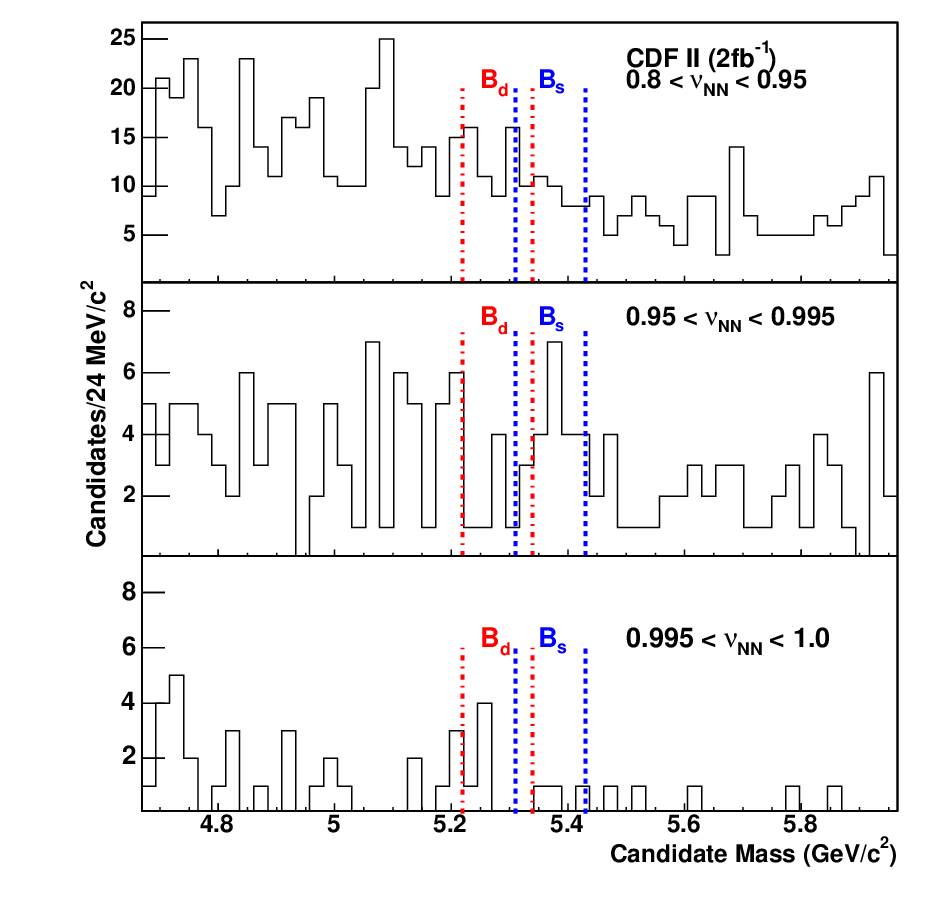
The FCNC decays $B^{0}_{s}(B^{0})\rightarrow\mu^{+}\mu^{-}$ occur in the standard model only through higher order diagrams. The expectations for the branching fractions are $BR(B^{0}_{s}\rightarrow\mu^{+}\mu^{-})=(2.42\pm 0.54)\times 10^{-9}$ and $BR(B^{0}\rightarrow\mu^{+}\mu^{-})=(1.0\pm 0.14)\times 10^{-10}$ [17] which are one order of magnitude smaller than the current experimental sensitivity. In SUSY models diagrams including sypersymmetric particles can increase these branching fractions at large $tan(\beta)$ [18], and also at small $tan(\beta)$ [19]. The new measurement uses 2 fb^-2 and the sensitivity is further improved by using an enhanced muon selection, and performing the search in a two dimensional grid in dimuon mass and neural network space. The discriminating variables used in the analysis include the measured proper decay time, $\lambda$, the proper decay time divided by the estimated uncertainty, $\lambda/\sigma_{\lambda}$, the 3D opening angle between the dimuon momentun and the displacement vector between the primary vertex and the dimuon vertex, $\Delta\Theta$, and the B-candidate track isolation, $I(B)$. To enhance signal and background separation a neural network discriminant is constructed, using all the discriminating variables except $m_{\mu\mu}$. The network is trained using MonteCarlo simulated $B^{0}_{(s)}$ events for signal and mass sidebands events for background. The mass search regions are $5.310<m_{\mu\mu}<5.430$ GeV/c² for the $B^{0}_{s}$ and $5.219<m_{\mu\mu}<5.339$ GeV/c² for the $B^{0}$, which approximately correspond to $\pm 2.5\sigma_{m}$ ($\sigma_{m}=24$ MeV/c²). The $B^{0}_{s}\rightarrow\mu^{+}\mu^{-}$ branching fraction is determined relative to the $B^{+}\rightarrow J/\psi K^{+}$ signal. Relative geometric acceptances and analysis efficiencies are estimated using MonteCarlo. The expected background is due to the contributions of the combinatorial continuum and from the $B^{0}_{(s)}\rightarrow h^{+}h^{{}^{\prime}-}$ decays.The contribution from the combinatorial is estimated by linearly extrapolating from the sideband region to the signal region. The contribution from $B^{0}_{(s)}\rightarrow h^{+}h^{{}^{\prime}-}$ decays is estimated to be one order of magnitude smaller than the conbinatorial background. Using an a priori optimization procedure, it was found that subdividing the signal region into several bins in mass and in the neural network variable improves the sensitivity of the analysis relative to using a single bin. The backgrounds, efficiencies and limits are computed in each bin separately. Figure 3 shows the $\mu^{+}\mu^{-}$ mass distribution for three different ranges of the neural network variable. We extract the following limits $BR(B^{0}_{s}\rightarrow\mu^{+}\mu^{-})<5.8(4.7)\times 10^{-8}$ at 95(90) % C.L. and $BR(B^{0}\rightarrow\mu^{+}\mu^{-})<1.8(1.5)\times 10^{-8}$ at 95(90) % C.L., which place further constraints on new-physics models [18][19].

CDF has measured the $B^{+}_{c}$ lifetime in 1 fb^-1 of inclusive $J/\psi\rightarrow\mu^{+}\mu^{-}$ data using the $B^{\pm}\rightarrow J/\psi l^{\pm}X$ decays, where $l$ can be an electron or a muon and $X$ are unmeasured particles. To measure the lifetime, we reconstruct a per event lifetime defined using variables measured in the transverse plane. Since not all the decay products of the $B_{c}$ decay are identified, we define a

from which we can obtain the true $B_{c}$ lifetime by defining a factor $K$, determined using MonteCarlo, where $ct=Kct^{*}$. The $B_{c}$ signal is reconstructed by selecting dimuon events with a di-muon mass falling within $\pm 50$ MeV/c² window around the $J/\psi$ mass, and requiring the presence of a third lepton forming a vertex with the $J/\psi$ candidate. Most $B_{c}$ signal is expected in the window with $4.0<m_{J/\psi l}<6.0$ GeV/c². The broad mass peak includes also significant amount of background, mainly due to events with a $J/\psi$ from $b\overline{b}$ and $c\overline{c}$ and an additional hadron which fakes a muon by punching through to the muon chambers, or an electron by leaving a signature in the calorimeter compatible with an electron, to events from the continuum background for $J/\psi$ with a third lepton, to $b\overline{b}$ events with a $J/\psi$ froma $b$-quark jet and a lepton from the other b, or events where conversions produce electrons which produce a $B_{c}$ candidate when paired to a $J/\psi$. Each of these background sources are estimated by using control samples and simulation. The fit of the $ct^{*}$ distributions is performed separately in the $J/\psi l$ and $J/\psi e$ decay modes, using likelihood functions (Figure 4 and 5). The combined result is $c\tau=142.5^{+15.8}_{-14.8}(stat.)\pm 5.5(syst.)$ $\mu$m, where the largest contributions to the systematic error is due to the resolution function and to the uncertainty on the silicon alignment.

A new CDF analysis has measured the $B^{0}_{s}$ lifetime using 1.3 fb^-1 of data reconstructed as $B^{0}_{s}\rightarrow D^{-}_{s}(\phi\pi^{-})\pi^{+}$ and $B^{0}_{s}\rightarrow D^{-}_{s}(\phi\pi^{-})\rho^{+}(\pi^{+}\pi^{0})$, where the $\pi^{0}$ is not reconstructed. The analysis reconstructs about 1100 fully reconstructed $B^{0}_{s}\rightarrow D^{-}_{s}(\phi\pi^{-})\pi^{+}$ candidates and a similar number of partially reconstructed $B^{0}_{s}\rightarrow D^{-}_{s}(\phi\pi^{-})\rho^{+}(\pi^{+}\pi^{0})$ decays. The increased statistics has an uncertainty due to the missing tracks or misassigned masses, but it can be properly accounted for and folded into the likelihood formulation. The lifetime fit of the $B^{0}_{s}$ meson is determined from two fits done sequentially. The first fit is of the reconstructed mass of the $B^{0}_{s}$ and it determines the relative fractions of the various decay modes and backgrounds. The second fit is of the proper decay time of the $B^{0}_{s}$ candidates and uses the fractions determined with the mass fit (Figure 6). The analisys determines $c\tau=455.0\pm 12.2(stat.)\pm 7.4(syst.)$, where the main systematics are due to the background model and to the uncertainty in the measurement of the fractions of the several contributions, to the uncertainty of the shape of the MonteCarlo $p_{T}(B^{0}_{s})$ distribution and to the silicon detectors alignment.

CDF has also performed analyses in the field of CP violation using hadronic decays reconstructed in 1 fb^-1 of data. A first analysis uses the $B^{-}\rightarrow D^{0}K^{-}$ modes, which allow a theoretically-clean extraction of the CKM angle $\gamma$ by a variety of methods, depending on the involved specific $D^{0}$ decay mode [20][21] [22][23]. These methods require no flavor tagging or time-dependent measurements and use only charged particles in the final state, which makes them well suited for a hadron collider environment. By using the data collected by the hadronic trigger we have reconstructed the modes where the $D^{0}$ decays to either $K^{-}\pi^{+}$ (flavor eigenstate) or $K^{-}K^{+}$, $\pi^{-}\pi^{+}$ (CP-even eigenstate). The relevant modes are separated from the larger $B^{-}\rightarrow D^{0}\pi^{-}$ modes by using a likelihood fit which exploits the kinematic differences among the decay modes and the particle identification information provided by the specific ionization in the drift chamber. The most relevant result of this analysis is the first measurement at a hadron collider of the direct CP asymmetry in the $B^{-}\rightarrow D^{0}_{CP+}K^{-}$ decay mode, $A_{CP+}=0.37\pm 0.14(stat.)\pm 0.04(syst.)$, which is in good agreement with the measurements performed at the $\Upsilon(4S)$ and has a comparable resolution. The analysis measures also other decay parameters useful to improve the determination of the CKM angle $\gamma$.

CDF has also performed a first measurement of CP-violating asymmetries and branching fractions of $\Lambda^{0}_{b}$ charmless two-body decays. These decays in a proton and a charged kaon or pion may show significant CP-violating asymmetries, of the order of 30 %. A measurement of these asymmetries may be useful to allow or rule out some extensions of the standard model [24][25]. The analysis uses the same general framework used for the measurement of two-body charmless decays of the B mesons, reported in [26]. An unbinned maximum likelihood fit, using kinematic information as well as particle identification information from the specific ionization measurement in the drift chamber, is used to measure the different components of the $\Lambda^{0}_{b}$ signal. These variables allow also to separate the $\Lambda^{0}_{b}$ from the $\overline{\Lambda}^{0}_{b}$ decays, thus allowing for a measurement of the direct CP asymmetry. The necessary corrections which take into account detector acceptance effects and trigger and offline selection efficiencies are determined from control samples and from simulated samples. Figure 7 reports the di-hadron mass distribution reconstructed in data in the $\Lambda^{0}_{b}$ window. We have measured $A_{CP}(\Lambda^{0}_{b}\rightarrow p\pi^{-})=0.03\pm 0.17(stat.)\pm 0.05(syst.)$ and $A_{CP}(\Lambda^{0}_{b}\rightarrow pK^{-})=0.37\pm 0.17(stat.)\pm 0.03(syst.)$

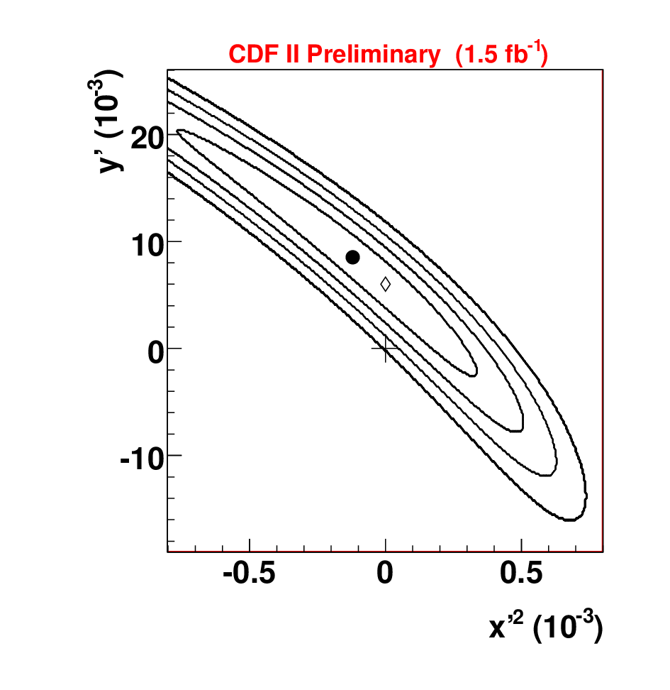
The recent evidence for $D^{0}$ mixing has been found in two different types of measurements. The BELLE Collaboration found direct evidence of a longer and shorter lived $D^{0}$ meson [27], the BaBar Collaboration found a difference in decay time distribution for $D^{0}\rightarrow K^{+}\pi^{-}$ compared to that for $D^{0}\rightarrow K^{-}\pi^{+}$ [28]. CDF has performed a measurement comparing the decay time distribution for $D^{0}\rightarrow K^{+}\pi^{-}$ compared to that for $D^{0}\rightarrow K^{-}\pi^{+}$. The ratio $R(t)$ of $K^{+}\pi^{-}$ to $K^{-}\pi^{+}$ can be expressed as a simple quadratic function of proper time $t$ under the assumption of CP conservation and small values for the parameters $x$ and $y$ [29], where the parameter $x$ is defined in terms of the mass difference $\Delta m$ between the heavy and light mass eigenstates and the parameter $y$ involves the width difference $\Delta\Gamma$ between these states. The CDF measurement uses 1.5 fb^-1 of data collected by the hadronic trigger. We reconstruct the Cabibbo-favored decay chain $D^{*+}\rightarrow D^{0}\pi^{+}$, with $D^{0}\rightarrow K^{-}\pi^{+}$ called “right sign” and the corresponding “wrong sign” and the selection cuts are chosen as to maximise the significance of the wrong sign signal. The ratio of wrong sign to right sign $D^{*}$ is determined by dividing the time distribution in bins. The distribution is fit to a parabola, related to the mixing parameters (Figure 8). The uncertainty on the mixing parameters includes effects from statistical fluctuations, uncertainties from the signal and background shapes and the corrections due to charm mesons from B decays. A Bayesian method is used to get the probability for different mixing parameters values. Contours containing the highest probability points are shown in Figure 9. The no-mixing point lies outside the contour equivalent to $3.8\sigma$ standard deviations, which is evidence of chamr mixing.

CDF has also searched for the rare $D^{0}\rightarrow\mu^{+}\mu^{-}$ decay, which is suppressed by the GIM mechanism in the standard model which predicts a branching fraction of the order of $10^{-13}$ [30], with possible enhancements of seven orders of magnitude in R-parity violating SUSY models. The CDF anaysis has been performed with 360 pb^-1 of hadronic data and follows the same strategy as in the previous CDF measurement [31]. The two-track candidates are reconstructed with the $\mu^{+}\mu^{-}$ mass hypothesis, and the $D^{*-}$ tag mass-difference is applied to reduce the combinatorial background. By using the well known $D^{0}\rightarrow\pi^{+}\pi^{-}$ decay mode as a normalisation mode, the analysis set the limit $BR(D^{0}\rightarrow\mu^{+}\mu^{-})<0.43(0.53)\times 10^{-6}$ at the 90(95) % C.L.

In this paper we have reviewed the current CDF hot topics in the fields of $b$ and $c$ physics. Most current CDF physics results are producd with 1-2 fb^-1. With the already collected 3.5 fb^-1 and the total 6 fb^-1 expected by the end of the year 2009, CDF expects to increase signficantly the number and the quality of the physics results in these sectors.

References

- [1] D. Acosta et al., the CDF Collaboration, Phys. Rev. D 75, 012010 (2007).
- [2] A. Sill et al., Nucl. Instrum. Meth. A530:1 (2004).
- [3] T. Affolder et al., Nucl. Instrum. Meth. A526:249 (2004).
- [4] D. Acosta et al., Nucl. Instrum. Meth. A518:605 (2004).
- [5] L. Balka et al., Nucl. Instrum. Meth. A267:272 (1988). M. Alborw. et al., Nucl. Instrum. Meth. A453:84 (2000).
- [6] G. Ascoli et al., Nucl. Instrum. Meth. A268:33 (1988).
- [7] E. J. Thomson et al., IEEE Trans. on Nucl. Sc. vol. 49, n. 3 (2002).
- [8] A. Abulencia et al., IEEE Trans. Nucl. Sci. 55, 126-132 (2008).
- [9] A. Bardi et al., Nucl. Instrum. Meth. A485:178 (2002).
- [10] W. Ashmanskas et al., Nucl. Instrum. Meth. A518: 532, (2004)
- [11] T. Aaltonen et al. (CDF Collaboration), Phys. Rev. Lett. 100, 121803 (2008).
- [12] V. M. Abazov et al. (D0 Collaboration), Phys. Rev. Lett. 98, 121801 (2007).
- [13] A. Zell et al., “SNNS, Stuttgart Neural Network Simulator, User Manual, Version 3.2” (University of Stuttgart, Stuttgart, Germany, 1994) (Computer Science Department, Report No. 6/94, 1994).
- [14] A. Abulencia at al. (CDF Collaboration) Phys. Rev. Lett 97, 062003 (2006).
- [15] A. Ali and F. Barreiro, Z. Phys. C 30, 635 (1986); M. Gronau, A. Nippe and J. L. Rosner, Phys. Rev. D 47, 1988 (1993); M. Gronau and J. L. Rosner, Phys Rev. D 49, 254 (1994).
- [16] G. J. Feldman and R. D. Cousins, Phys. Rev. D 57, 3873 (1998).
- [17] G. Buchalla and A. J. Buras, Nucl. Phys. B400, 225 (1993); A. J. Buras, Phys. Lett. B566, 115 (2003).
- [18] S. R. Choudhury and N. Gaur, Phys. Lett. B 451, 86 (1999).
- [19] R. Arnowitt et al., Phys. Lett. B 538, 121 (2002).
- [20] M. Gronau and D. Wyler, Phys. Lett. B 265, 172 (1991).
- [21] M. Gronau and D. London, Phys. Lett. B 253, 483 (1990).
- [22] A. Atwood, I. Dunietz and A. Soni, Phys. Rev. D 63, 036005 (2000).
- [23] D. Atwood, I. Duniets and A. Soni, Phys. Rev. Lett. 78, 3257 (1997).
- [24] R.Mohanta et al. Phys. Rev. D 63, 074001 (2001).
- [25] R. Mohanta et al. Phys. Rev. D 63, 056006 (2001).
- [26] A. Abulencia et al. Phys. Rev. Lett. 97, 211802 (2006).
- [27] M. Staric et al. (BELLE Collaboration), Phys. Rev. Lett 98, 211803 (2007).
- [28] B. Aubert et al. (BaBar Collaboration), Phys. Rev. Lett. 98, 211802 (2007).
- [29] B. Aubert et al. (BaBar Collaboration), Phys, Rev. Lett. 91, 171801 (2003).
- [30] G. Burdman et al., arXiv:hep-ph/0112235 v2 (March 2002).
- [31] A. Acosta et al., Phys. Rev. D 68, 091101 (2003).