Traffic of cytoskeletal motors with disordered attachment rates
Abstract
Motivated by experimental results on the interplay between molecular motors and tau proteins, we extend lattice-based models of intracellular transport to include a second species of particle which locally influences the motor-filament attachment rate. We consider various exactly solvable limits of a stochastic multi-particle model before focusing on the low-motor-density regime. Here, an approximate treatment based on the random walk behaviour of single motors gives good quantitative agreement with simulation results for the tau-dependence of the motor current. Finally, we discuss the possible physiological implications of our results.
pacs
05.40.-a, 87.16.A-, 87.16.Nn, 87.16.WdI Introduction
Active transport on a microscopic scale is one of the most important features of living organisms [1]. Transport of this kind is responsible for the functionality of eucaryotic cells and ultimately, via contraction of muscle cells, for the motion of organisms. Unsurprisingly, perturbations of the intracellular transport can lead to pathological conditions; for example, the role of molecular motors in sensory defects is discussed in [2]. Another example is Alzheimer’s disease in which the breakdown of axonal transport, taking place before plaque formation can be observed, has been reported for transgenic mice [3]. In particular, there is experimental evidence that an over-expression of the linker-protein tau may reduce the tubulin affinity of kinesin motors [4, 5]. Therefore the investigation of the basic mechanisms of intracellular transport is not merely of theoretical interest.
Studies of molecular motors discuss, e.g., the necessary prerequisites for the directed stochastic motion of single motors or the cooperative dynamics of many motor proteins attached to a single cargo [6, 7, 8, 9]. From a theoretical point of view these cases can be considered as single self-driven particles. Although the characterization of the individual motions is of high relevance for many biological and biophysical systems, often intracellular transport is carried out by several self-driven particles. Systems of this kind show generic many-particle behaviour [10]. Focusing on the many-particle features of intracellular transport, it is sufficient to consider an effective motion for the molecular motors on the filaments. Molecular motors move generically unidirectionally and stepwise [11]. The size of the steps is, in general, load dependent and given by multiples of the structural unit length of the filament. Another important feature of the motor dynamics is its stochastic nature, i.e., binding and unbinding as well as the movements on the filament are random events which are described by rates.
These properties of the dynamics suggest that intracellular transport can be described by models that are in close analogy to the asymmetric exclusion process (ASEP)—a one-dimensional lattice model for interacting self-driven particles [12]. Compared to the ASEP, one has to account for the finite “run length” of molecular motors, i.e., the absence of particle conservation on the track. Various models of this kind have been proposed, see e.g. [13, 14], which show particularly interesting many-particle effects on open lattices. The absorption and desorption of particles leads to the formation of localized high and low density domains. This modelling approach is very flexible and can be easily generalized, for example, in order to explain the results of in vitro experiments [10]. For recent reviews treating statistical mechanics descriptions of intracellular traffic, see e.g., [15, 16, 17].
In the present work we discuss the influence of a second type of particle which alters the attachment rates of the self-driven particles in different one-dimensional environments. The model under investigation aims to reproduce the generic features of the kinesin dynamics on microtubules for different concentrations of tau. In addition to shedding light on this specific biological situation our study contributes to the understanding of disorder in driven many-particle systems.
The rest of the paper is organized as follows. In Sec. II we review the lattice-based model for intracellular transport introduced by Klumpp and Lipowsky [18] and discuss simulation results obtained by generalizing it to include the effect of tau. Then, to gain further insight, we introduce in Sec. III a somewhat simplified model which retains the key features of the problem but is more amenable to analytical treatment; we also discuss some limits in which this model is exactly solvable. In Sec. IV we address the biologically important question of how the mean current and its fluctuations depend on the concentration of tau. A random walk treatment for single motors leads to predictions for the low-motor-density regime of the multi-particle model which are in good agreement with simulation. Finally, in Sec. V, we conclude by discussing the possible physiological relevance of our results and potential generalizations to more realistic models.
II From biology to simulation
In this section we outline how the complex biological system of interest can be represented by a lattice-based model amenable to simulation. Specifically, we build on the work of Klumpp and Lipowsky [18], generalizing their model to include tau proteins and presenting specimen simulation results. This is in the spirit of a now well-established approach to complex systems whereby one considers simple models in order to help understand phenomena and mechanisms which may also occur in more realistic situations. Indeed, we will pursue this approach further in the following section in which we discuss an even more simplified model allowing for analytical treatment.
II.1 Model of Klumpp and Lipowsky
As discussed in the introduction, motor proteins carry out directed walks (i.e., active transport) on the filaments of the cytoskeleton. In the context of neuronal transport, we are particularly interested in the motion of kinesin along axon microtubules (composed of repeating tubulin subunits) [19]. The stepwise structure of such movement naturally suggests using a one-dimensional (1D) lattice model with lattice-spacing equal to the step size [11]. We assume that the size of the kinesin molecules is comparable to this unit lattice spacing; the mutual exclusion of motors is then imposed by preventing double occupancy of any one site. An obvious starting point for modelling the dynamics is the prototypical asymmetric simple exclusion process in which particles hop to vacant nearest neighbours with some preferred direction (for a review of this exactly-solvable model, see [20]). In fact “backward” steps for kinesin are extremely rare so it suffices to consider the totally asymmetric version in which particles can only hop in one direction.
Since kinesin motors typically detach from the microtubule after a certain number of steps (“run length”) and diffuse in the surrounding medium before reattaching, one needs to extend the standard ASEP picture. A simple choice is to impose the same lattice structure and exclusion rules off the filament but allow the molecules to move symmetrically there. The association onto and dissociation from the track is governed by explicit rates (typically the dissociation rate is comparatively small so that a single motor can make many steps before detaching).
Klumpp and Lipowsky embed this lattice model in a cylindrical geometry with directed motion along a 1D track located at the symmetry axis of the cylinder and undirected motion (diffusion) elsewhere. Of course, this is a considerable simplification compared to a real nerve cell which contains a bundle of parallel microtubules. However, it is expected to reproduce qualitatively the main features of unidirectional transport (and could readily be computationally extended to the case of several parallel tracks). Another important question concerns the boundary conditions at the ends of the cylinder. In [18] both periodic and open boundary conditions are considered; in the former case, the current-density relation is obtained and, in the latter, the phase diagram.
II.2 Effect of adding tau
In this subsection we generalize the above-described model of Klumpp and Lipowsky to include the effect of tau proteins. The interested reader is referred to [21, 22] for details of the structure of tau and its interaction with tubulin. Here we merely note that tau molecules “decorate” the microtubule (indeed they are believed to play a role in stabilizing it) but do not undergo active transport along it. We can therefore incorporate them in our model by introducing a second species of particle which is allowed to diffuse in the bulk, and absorb/desorb with certain rates but not to move along the track itself. Figure 1 summarizes the various processes now incorporated in the model.

In the present work we restrict ourselves to periodic boundary conditions. Although one expects that real nerve cells are better described by open (or half-open) boundary conditions cf. [23], studying the simpler case of periodic boundary conditions already gives information about bulk effects. We further justify our choice by remarking that the finite run lengths of the molecular motors might be expected to reduce the dependence of currents on the filament boundary conditions.
To complete our description of the model we must specify the details of the tau interactions. Firstly we note that tau molecules are relatively small compared to the motor-cargo complex. Single motor in vitro experiments [5] also indicate that the presence of tau does not affect the speed of kinesins along microtubules or their run length (probably because kinesin and tau have different binding sites [22]) but does lead to a significant reduction in the attachment rate.
In the present simulation model, we therefore neglect tau-tau and tau-kinesin exclusion effects (i.e., each unit lattice step can contain one or more tau particles, regardless of the presence or absence of a kinesin motor). However, the crucial point is the effect of tau on the kinesin dynamics. In vivo experiments [4] are complicated by the fact that many motors can be attached to a single cargo but also suggest that one effect of tau is a decrease in the motor attachment rate (especially for kinesin). Hence, in the present model, when one or more tau molecules occupies a site on the track the rate for absorption of a kinesin is reduced.11 1 Note that some aspects of our model are similar spirit to the discussion of crowding by another molecular species which already appears in [24]. However, the specifics are rather different—in particular, in that work, there is exclusion of motors by the “obstacles” and the obstacles can also be actively unbound by processive motors.
The description above furnishes a model which retains the key features of the biological system but can be implemented simply in numerical simulation. In principle, one can try to match the parameters of the model (lattice spacing, rates, etc.) to those known from experiments in order to obtain quantitatively meaningful results. We carried out simulations using relative values for the kinesin rates based on data for the case without tau in [13].22 2 The rates are equivalent to probabilities per timestep; for comparison with real data, normalization of the timescale would then be achieved by associating the length of each timestep with a physical time unit. Specifically an unbound kinesin could hop to a neighbouring empty filament site with rate 0.0083 which was identical to the hop rate between a pair of empty bulk sites (i.e., the binding probability was one). The rate for a forward step on the filament was 0.0099 and the desorption rate from the filament to each of the four adjacent unbound lattice sites was . The tau molecules were (arbitrarily) set to diffuse twice as fast as the motors and had absorption and desorption rates, 0.03 and respectively, which are consistent with data from FRAP (Fluorescence Recovery After Photobleaching) experiments [25]. Note the high affinity of tau for the microtubule which leads to significant tau coverage on the filament even for low global densities.
In order to illustrate the possible effect of tau on kinesin binding and transport, we reduced the kinesin adsorption rate by a factor of one hundred in the presence of tau. This value arguably overestimates the impact of tau in real systems. (In [5] it was shown that the binding rates depend on the ratio between tau and kinesin concentration; for the highest concentration of tau used in that experiment the binding rates were reduced by a factor of five.) However, we expect a stronger influence of tau in living cells since the typical run length of the molecular motors must be shorter than in in vitro assays, due to the bidirectionality of the transport and the dynamics of the filament.
Figure 2 shows simulation results for the current along the track versus bound kinesin density for different values of global tau density.

One sees from these results that increasing the density of tau reduces the height of the maximum and shifts it to higher kinesin densities. The average current is reduced for low densities of kinesin but increased for high densities. Furthermore, the simulation results cannot be reproduced by a simple mean-field approximation which indicates the significance of correlation effects. Indeed explicit measurements of the kinesin pair-correlation functions show the existence of long-range correlations. To explore the tau-induced effects analytically, in the next section we present and discuss an even simpler model.
III Minimal model
In order to elucidate the mechanisms leading to the features observed in the simulations described above, we now introduce a simpler model which can be treated analytically in certain limits. Specifically, instead of the cylindrical geometry we consider a two-lane system (analogous to the “two-state approximation” of [18]) with somewhat simplified effective dynamics for the tau particles.
Note that this is now a stylized “toy” model designed to yield increased understanding but not quantitative agreement with experimental results. We further remark that simple two-lane models have previously been used as crude representations of vehicular traffic and are of more general interest in building up our knowledge of non-equilibrium statistical physics, see e.g., [26, 27, 28, 29]. In the following analysis we mainly use the language of physics (“lattice sites”, “particles”, etc.) whilst keeping in mind the original biological motivation. The physiological significance of our results will then be discussed in more detail in Sec. V.
III.1 Model definition
We consider a two-lane lattice gas model with periodic boundary conditions, as shown schematically in Fig. 3. Here the lower lane represents a microtubule (MT) filament and the upper one the surroundings. The model contains two species of particles representing kinesin motors (K) and tau proteins (). We denote the occupation number for K-particles on the th site in the lower or upper lanes by or respectively (where the letters denote “bound” and “unbound” in allusion to the biological context). The -particles are found only in the lower lane (see below) with occupation number . The total number of each kind of particle is conserved and a hard-core interaction prevents more than one of each species on a given site, i.e, the site occupation numbers can take only the values 0 or 1. The dynamics of the model (defined in continuous-time) are motivated by the biological picture, as will be explained below.

We first make some remarks on the behaviour of the -particles. After the discussion of Sec. II the exclusion condition may seem very unrealistic. However, for the kinesin transport the relevant question is whether a given location on the microtubule contains at least one tau molecule (in our simplified description the number of such molecules is irrelevant). It therefore seems reasonable to reduce the state-space and consider only “tau-occupied” and “tau-empty” sites, in other words the presence or absence of an effective -particle. Similarly, we argue that tau desorption, diffusion and absorption can be represented by an effective undirected motion along the track.33 3 Of course, this simplified representation would be inappropriate for addressing questions about the distribution and dynamics of the tau particles themselves. With respect to properties of the kinesin transport, the validity of the approach will later be further justified by the similarities between simulation results from this minimal model and from the full model of Sec. II. Hence, in our simplified model, the -particles undergo a symmetric exclusion process (SEP) in the lower lane. Specifically, a -particle at site in the lower lane hops randomly (after an exponentially distributed waiting time) to one of the nearest-neighbour sites or . The rate for each of these moves is if the destination site is vacant and zero otherwise. It is clear that the average occupation number in the steady state is site-independent. [Here, as throughout the paper, we use angular brackets to denote an average over stochastic histories.]
K-particles can occupy sites in both the lower lane and upper lane (corresponding to kinesin motors being bound or unbound respectively). Along the lower lane the dynamics is given by a totally asymmetric exclusion process with rate for rightward hops. Diffusion of motors in the surroundings of the filament, is represented by a symmetric exclusion process in the upper lane with rate . The key feature of the model (reflecting the underlying biology) is that the coupling of these two processes depends on the local density of -particles. Specifically, a K-particle in the upper lane hops to a K-vacant neighbouring site in the lower lane with rate if the destination site is not occupied by a and with a (reduced) rate if there is a there. In contrast, a K-particle in the lower lane moves to a vacant neighbouring site in the upper lane with rate , regardless of the presence or absence of .
To summarize, our model is defined by the possible moves (and corresponding rates) listed in Table 1.44 4 Note that we sometimes use the generic for statements which apply separately to all three inter-lane rates , , .
| Move | Rate | Biological interpretation |
|---|---|---|
| Effective diffusion of tau along MT | ||
| Directed motion of kinesin along MT | ||
| Diffusion of kinesin in surroundings | ||
| Detachment of kinesin from MT | ||
| Attachment of kinesin in absence of | ||
| Attachment of kinesin in presence of |
Even this simple model is difficult to treat analytically since the K-particles experience a dynamic disorder due to the interaction with . For reviews of earlier work on disorder in driven diffusive systems see, e.g., [30, 31]. For a disordered asymmetric exclusion process with non-conserving sites, Evans et al. [32] were able to solve the steady state exactly in two limits. In a similar spirit, we treat below some tractable limits of the present model as well as discussing more qualitatively the general case.
III.2 Tractable limits
For a fixed density of -particles, the behaviour of the system is characterized by plotting the stationary current along the lower lane against the density of K-particles. In this subsection we show how this “fundamental diagram” can be calculated exactly in certain limits and compare the -induced changes with the observations from the more realistic model in Sec. II.
III.2.1 Pure case
In the absence of (i.e., ), the model is exactly solvable as shown by Klumpp and Lipowsky [18]. The steady state is a product state with site-independent K densities in lower and upper lanes and . Since this stationary state has no correlations between sites, these densities obey the mean-field equation
| (1) |
which corresponds to the absence of a net current between the two lanes. Combined with the expression for the (known) total motor density
| (2) |
this yields a quadratic equation for which can be solved explicitly. The mean current along the track is then obtained as
| (3) |
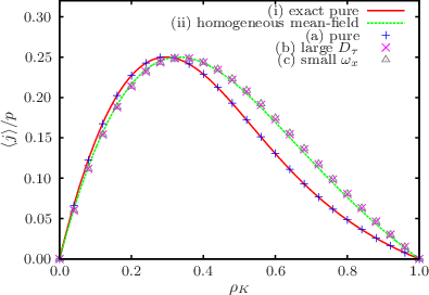
In Fig. 4 we plot against the total motor density ; note that in the pure case the shape of this “fundamental diagram” is completely determined by the ratio of absorption and desorption rates .
III.2.2 Fast diffusion of -particles
If the -particles diffuse infinitely fast relative to the movement of the K-particles then there is no possibility for correlations to build up in the system and the presence of the -particles merely alters the average absorption rate. Hence in the limit (with the other rates all finite), one expects that the stationary state is still described by the simple mean-field theory (i.e., with uncorrelated homogeneous site densities) with an effective absorption rate given by
| (4) |
This expectation is confirmed by the simulation results shown in Fig. 4. Notice that the effect of the introduction of (with ) is to shift the position of the maximum towards higher K-densities.
As an aside, we note that the same mean-field solution is found for any value of in the limit of vanishing coupling between the lanes, (i.e., , , ) with the ratios and constant. In this limit the time between each lane-changing event tends to infinity so that after each such event the K-density profiles in the lower and upper lane relax to the spatially-uncorrelated homogeneous case and we again recover the mean-field result with effective rate given by (4) (see again the simulation results in Fig. 4).
III.2.3 Slow diffusion of -particles
Let us now consider the quenched disorder limit, i.e., . In this case, the time between movement of -particles tends to infinity and between these events the system relaxes to a quasi-stationary state with site-dependent densities of K-particles. There is a growing body of literature discussing lattice gas models with quenched spatial disorder but analytical progress is difficult even for the usual single-lane ASEP (see, e.g., [33, 34, 35, 36, 37]). For our two-lane model, we focus here on two limiting cases where the analysis again becomes relatively straightforward; comparison with simulation is shown in Fig. 5.

Firstly, we consider taking followed by whilst holding the other ratios between rates constant. Here the density profile in the lower lane relaxes rapidly to stationarity between each hopping event in the upper lane. In other words, the profile in the lower lane is that of a homogeneous ASEP (constant density ) whereas the density in the upper lane is inhomogeneous and determined by the local absorption and desorption rates. Specifically, there are two distinct unbound densities and corresponding to the absence and presence of respectively. These densities must obey the relations
| (5) | |||||
| (6) |
and the equation for total K-particle density becomes
| (7) |
Substituting (5) and (6) into (7) gives
| (8) |
For fixed this is a cubic equation for ; numerical solution followed by substitution into (3) yields a current in good agreement with simulation.55 5 Even better agreement would presumably be obtained for smaller relative to but then longer simulation times would be required to reach the steady state.
Secondly we consider the case where and then (again with the other ratios between rates held constant). Here the density in the upper lane relaxes to that of a homogeneous SEP (constant density ) and the density in the lower lane is inhomogeneous with two possible values and given by the local absorption and desorption rates via
| (9) | |||||
| (10) |
These densities must satisfy
| (11) |
leading to
| (12) |
After solving this cubic equation for one can obtain the two bound densities via (9) and (10). The current along the lower lane is of order and its average value can be calculated by using the probabilities to find a -particle at either end of a given bond:
| (13) |
Of course, on very long timescales the positions of the -particles and hence the local densities of K-particles will change. However, the system will rapidly relax to a new quasi-stationary state which, on average, has the same K-current (as follows from conservation of -particle number). The prediction of (13) is again well-supported by simulation even for parameter values, which for computational efficiency, are still relatively far from the limiting case; see Fig. 5.
III.3 Intermediate parameters
All the limits treated in the previous subsection correspond to cases where in the (quasi-)stationary state there are no correlations between the occupations of different sites (i.e., they are situations which can be described by forms of mean-field theory). However, we emphasize that this is not expected to be the case for general choices of rates. In this subsection we present illustrative simulation results for intermediate parameters—see Fig. 6.

The relative values chosen are inspired by the biological context although we make no attempt to quantitatively match our simple model to real data. Specifically, the bulk diffusion and absorption rate are large compared to the hopping rate on the track but the desorption rate is small. The presence of tau strongly reduces the absorption probability () [5] while the effective diffusion rate for tau is rather small. The simulation data shown in Fig. 6 shows that, just as in the limiting cases discussed in III.2.2–III.2.3, there is a shift in the position of the maximum towards higher K-densities (compared to the pure case). However, significantly, there is also a decrease in the height of this maximum. We remark that a shift in the maximum, a reduction in its height and significant correlations were all observed in simulations of the more realistic model in Sec. II.
From a theoretical point of view, the shape of the fundamental diagram is interesting (in particular, the effect of tau on the position and height of the maximum). Physiologically however, one expects the number of kinesin motors to be approximately constant, and thus a more relevant question is the dependence of current on tau concentration at a fixed low density of motors. Of course, it is possible to analytically obtain this dependence in the tractable limits discussed above. For more “realistic” intermediate parameters, a good approximate description in the low K-density regime can be obtained by considering the random walk properties of single motors which is the approach we choose to pursue in the following section. To simplify the analysis while retaining the most important features we henceforth set and .66 6 We can appeal to physical intuition and simulation results (cf. Fig. 5–6) to support the assertion that, with respect to the current of -particles, there is no singular behaviour at this limit.
IV Tau-dependence of current
IV.1 Single-motor properties
In this subsection we show how the properties of a single motor (or equivalently an ensemble of non-interacting motors) can be analytically understood through a random walk picture. This facilitates an investigation of the effect of tau on the average velocity and diffusion constant of the motor (or equivalently the mean and variance of the current). Such a single-particle random walk approach (cf. [38, 13, 39]) is relevant for in vitro experiments involving individual motors but, as we shall see in IV.2, also gives valuable information about the low-motor-density limit of the interacting-motor problem.
IV.1.1 Probability distributions, large deviations
Let us start by considering a single motor moving in the quenched disordered landscape defined by Fig. 3 with and . We are interested in the distribution of the total number of steps made by a single motor in the lower lane over some time period (i.e., the integrated current in time ). Now it is obvious that, if the motor spends a fraction of its time in the lower lane, then has a Poisson distribution with mean , i.e.,
| (14) |
or equivalently the observed time-averaged current has the distribution
| (15) |
The full distribution of is then obtained by averaging over all possible values of , i.e.,
| (16) |
where is the distribution of the fraction of time (from a total ) spent in the lower lane. Our central task is thus to calculate this distribution and hence obtain the distribution of . We note that is expected to have a large deviation form
| (17) |
and that knowledge of the large deviation function gives the asymptotic behaviour of all moments of the distribution.
Before showing how to obtain approximately in the disordered case, we first digress to discuss the pure result corresponding to . In this case, the upper and lower lanes form an effective two-state Markovian system with rates and for transitions between the states. It can then be shown exactly that the distribution of the total fractional time in the lower (bound) state is given by [40]
| (18) |
where is the Dirac delta function, and are Bessel functions, and are the probabilities to find the motor in the bound and unbound states respectively and
| (19) |
Furthermore, it is trivial to show that
| (20) |
The expression (18) can then be substituted into (16) and numerical evaluation of the resulting integral agrees with the current distribution obtained by simulation (not shown). In the long-time limit (18) reduces to a Gaussian [41].
IV.1.2 Disordered model as trapping problem
In the disordered case (non-zero density of tau) the upper and lower lanes no longer form an effective two-state Markovian system (the average rate for escape from the upper lane is dependent on the occupation time, since for longer times the particle is more likely to be found trapped in long tau-decorated regions). However, for a two-state non-Markovian system, it can be shown [42] that the asymptotic distribution of occupation times is still Gaussian with the fraction of time in the lower lane having mean
| (21) |
and variance given by where
| (22) |
Here () and () are the mean and variance of the sojourn time distribution in the upper (lower) lane. Since the rate for exiting the lower lane is always we have
| (23) |
and the only remaining difficulty is to calculate the equivalent quantities for a sojourn in the upper lane. Obviously, , and hence and are functions of but for simplicity we suppress this dependence notationally.
Now, focusing in on the upper lane, we see that a K-particle performs an ordinary random walk (with hopping rate ) in regions of sites occupied by tau. When it reaches a site without tau, it has a probability to be “trapped” and move to the lower lane. For several decades such one-dimensional trapping problems have been extensively analysed in the literature (see, e.g., [43, 44, 45] and references therein). In particular it can be shown (see, e.g., [46]) that the tail of the sojourn time distribution has a stretched exponential form due to the survival of particles in arbitrarily large trap-free regions. However, we are interested in the mean and variance which are not much influenced by the tail of the distribution. Here we show how, within certain approximations, these quantities can be calculated directly. Our approach is in the spirit of a continuous time-version of the method given in [47].
First we consider two traps separated by a “line segment” of length as shown in Fig. 7.

In other words, we have a tau-free site at followed by sites occupied by tau, followed by another tau-free site at . The time to reach one of the traps at either end starting from position is a random variable ; it can be shown by standard arguments [48] that its mean is given by
| (24) |
Note that this expression is invariant under the transformation as expected from the symmetric nature of the diffusion. We now make the important assumption that the distribution of entry points into the upper lane has a uniform distribution. This is expected to be a good approximation when the typical run length in the lower lane is large compared to the spacing of traps, i.e., when
| (25) |
Using , without subscript, to denote the time to absorption from a random initial position we then obtain
| (26) | ||||
| (27) |
Following [48], one can also write down expressions (see appendix) for the mean square first passage times and . Combined with a known distribution of traps (i.e., the distribution of lengths ), this is sufficient to obtain explicit expressions for the first two sojourn time moments in the case where the trapping probability is unity (i.e., ). However, for imperfect trapping one must allow for the possibility that the particle is not absorbed on its first visit to the trap. We now discuss two possible approximations which allow further analytical progress:
- 1.
In the “reflecting trap” or “decoupled-ring approximation” [43, 49] it is assumed that a particle which is not absorbed by a trap is always reflected back into the same trap-free line segment from which it came.77 7 A particle which enters the upper lane at a trap site is randomly assigned to the line segment to the left or the right. This simplifies the analysis by decoupling the tau segments between traps but at the expense of introducing an uncontrolled approximation. The approach is clearly exact in the case of perfect traps (i.e., in our model for ) but has also been shown to give good results for trapping probabilities smaller than unity [49].
- 2.
Another approach is to place each particle which escapes from a trap site on to the first site (i.e., ) in a line segment with length randomly drawn from the distribution of all possible lengths. Again this approximation is exact for . Furthermore, we might also expect it to be exact in the limit of zero-trapping probability () since in this case each particle explores the full distribution of tau line segments.
Whereas the first approximation treats the line segments as unconnected, the second assumes they are all interconnected, in the sense that a particle can escape from a trap into any line-segment (rather than just neighbouring segments as happens in reality). For intermediate trapping probabilities, we might expect the true distribution of first passage times to fall somewhere in between the predictions of these two limiting cases. The analytical approach proceeds in a similar way for both approximations; we give here the details for approximation 7, indicating only briefly the modifications necessary for approximation 2.
Let us start by considering a particle which enters the upper lane at a random position in a tau segment of length . The total sojourn time spent by the particle in the upper lane is a random variable given by the following sum
| (28) |
Here is the number of times the particle is reflected from the trap, is the time to reach the trap for the first time (from a random initial position), is the time spent at the trapping site on the th visit and is the time to return to the trap after escaping for the th time. Under approximation 1, the particle is always reflected back into the same line segment and . Averaging over stochastic histories then yields
| (29) |
where we have used the independence of the various random variables in order to factorize the expectation values.
Noting that the number of reflections has a geometric distribution given by
| (30) |
we immediately find
| (31) |
Furthermore the time spent at the trap is exponentially distributed with mean
| (32) |
Together with (24) and (27), this allows a complete determination of .
Next we note that the probability of entering the upper lane in a given line segment (i.e., a sequence of consecutive sites occupied by tau) is proportional to its length. Hence for a uniform distribution of -particles we should average over the distribution
| (33) |
The resulting infinite sum
| (34) |
contains summands proportional to with and evaluates to
| (35) |
The only difference in approximation 2 is that the lengths appearing in (28) are drawn from the distribution . After averaging over this distribution as well as the initial distribution one finds
| (36) |
In similar fashion one can obtain an expression for from (28). The resulting calculations are straightforward but tedious and are outlined for convenience in the appendix. Using approximation 7 one eventually obtains
| (37) |
Results (35) and (37) together with (21)–(23) finally determine the parameters of the asymptotic Gaussian form of .
IV.1.3 Results for velocity and diffusion coefficient
After the effort involved in finding the long-time behaviour of , it is comparatively straightforward to evaluate the integral (16)—one simply uses Stirling’s approximation for the factorials in the Poisson distribution and then employs a saddle-point treatment. This finally yields the large deviation function of the observed average current along the lower lane
| (38) |
where is the positive solution of the quadratic equation
| (39) |
The large deviation function gives knowledge of all cumulants of . In particular, we easily obtain the mean velocity
| (40) | ||||
| (41) |
and diffusion constant
| (42) | ||||
| (43) |
In fact, this is simply the expected result for the variance of a compound process. However, we emphasize that the large deviation expression (38) also gives complete information about the asymptotic behaviour of higher moments.
Using (21) and (22) for the bound-state occupation probability and its variance, we obtain explicit expressions for velocity and diffusion. Specifically, the observed average motor velocity along the lower lane in the presence of a quenched distribution of is given by (under approximation 1)
| (44) |
In Fig. 8 we compare the analytical predictions of both approximate schemes with simulation results for the mean velocity of a single motor.

We find that both approximations reproduce well the decrease of the average velocity with increasing tau concentration and that, as anticipated, the simulation results lie between the two curves.
Similarly the analytically-calculated diffusion constant compares well with simulation, as shown in Fig. 9.

In particular, we see that although the system is relatively robust to low concentrations of tau, for high concentrations there is a dramatic increase in the variance which could be physiologically significant.
In fact, it is perhaps more illuminating to consider the diffusion constant divided by the square of the velocity as shown in Fig. 10.

This defines a crossover timescale . For times less than , diffusive fluctuations dominate whereas for larger times the directed motion is dominant.
IV.2 Low motor density
The single motor calculations of the previous subsection can be used to give approximate results for the low-motor-density limit of the full model. The key observation is that, for realistic parameters, the total unbound density is much smaller than the total bound density (except for very close to unity). It is thus reasonable to neglect the exclusion interaction both in the upper lane and also for inter-lane moves. In other words we have an asymmetric exclusion process on the filament coupled to random walks (without exclusion) in the surroundings.
In this approximation one then assumes a homogeneous bound density given by
| (45) |
In other words a proportion of the total K-particles are expected to be in the lower lane (where is the bound-state occupation probability calculated for the single motor case). Assuming no correlations between the bound densities on neighbouring sites, the associated mean particle current is given by
| (46) |
As seen in Fig. 11,

this approach is a considerable improvement over the simple mean-field (i.e., neglecting all correlations and simply replacing by the effective absorption rate given by (4)) since it implicitly takes account of correlations between tau and unbound motor density. However, it still assumes an uncorrelated uniform density of bound motors (only expected to be a good approximation when many hops along the filament take place between absorption/desorption events). To test this assumption we plot, in Fig. 12,

averaged density profiles for the rate parameters used in Fig. 11 with . In fact there is significant spatial dependence in the bound density but the relative variation is much less than in the unbound density (where we find peaks corresponding to the trapping of particles in tau-occupied regions). As a quantitative comparison we remark that for the scenario shown in Fig. 12 the standard deviation of the lower-lane densities is approximately 0.14 of their mean (over 1000 lattice sites) whereas the equivalent ratio for the upper lane is about 0.84. For larger the run length of the molecular motors increases relative to the trap spacing so that the bound density becomes much more homogeneous while the unbound density is essentially unchanged (not shown).
Based on the single motor results we also expect high concentrations of tau to significantly increase the variance of the bound K-particle current. Indeed, this is observed in simulations as shown in Fig. 13.

For low tau-densities we see a plateau where the variance is dominated by that of the ordinary single-lane exclusion process, which can be calculated exactly [50, 12]. At a high tau concentration, a peak appears resulting from the inter-lane fluctuations (just as in the single motor case). It seems difficult to obtain the shape of this peak analytically since fluctuations along the lower lane and fluctuations between the lanes are not independent.
V Discussion
This work is concerned with the stochastic modelling of molecular-motor traffic inside cells. In particular, we were motivated by experimental observations of the influence of the linker protein tau on transport in axons [4, 5]. These experiments suggest that the primary effect of tau proteins is to reduce significantly the binding-affinity of the motor proteins rather than to alter their dynamics on the microtubules.
In order to model this situation, we extended an earlier lattice-based approach due to Klumpp and Lipowsky [18]. Specifically, whereas the original model contained only a single species of particles (representing kinesin motors), we introduced a second type of particle to represent the tau proteins. Following Klumpp and Lipowsky we modelled the axon in a simplified fashion using a one-dimensional track embedded in a cylindrical geometry. The dynamics of the model was defined to reflect the picture suggested by experiment so that the local presence of tau reduces the rate for kinesin particles to attach at a potential binding site but does not affect the rates for movement along the track.
Simulation results for this model show that for a wide range of parameters, the presence of tau causes only a marginal reduction in the maximum transport along the axonal filament. (This finding is consistent with the very recent results of [51].) However the position of the maximum is shifted to higher kinesin densities and for a given density of motor proteins one may observe a vigorous alteration of the flow. This result indicates that an overexpression of tau proteins may perturb the intracellular transport significantly. The central aim of the present work was to characterize and understand this disruption within simple models and thus gain tentative insight into possible mechanisms in the real biological context. (We have not attempted to make quantitative predictions and further work would be needed to determine to what extent our observations are seen in real physiological conditions.)
In this spirit, in order to analyse in more detail the origin of the transport disruption we further simplified the modelling approach by introducing a two-lane model, which is analytically treatable for selected, but generical, limiting cases. For the case of the pure model, i.e., the case without “-particles”, it is known that the stationary distribution is given by a product measure [18]. However, with the introduction of -particles, mean-field properties are only found in certain limits. For example, the case of fast diffusion of -particles can be described by introducing effective binding rates for the kinesin-particles.
A qualitatively different behaviour is observed if we consider slow diffusion of -particles. This corresponds to quenched disorder on the track leading to non-trivial density profiles of the “K-particles” which represent the motors. For arbitrary model parameters this limit is difficult to analyse. However, there are two limiting choices of motor rates which still yield a product measure for the motor distribution—these choices correspond to a space-dependent distribution of particles in one lane and a homogeneous distribution in the other. In these cases one observes that the position of the maximal current can be significantly changed by the -particles. A shift of the maximum to higher K-densities (for fixed -densities) is also a feature of simulation results for more general parameters. However, when correlations cannot be neglected one also sees a decrease in the height of the maximum. In these respects the simplified two-lane model reproduces to a large extent the properties of the full model.
In the context of the biological system, it is instructive to analyse the features of the model for a fixed density of motor proteins and different concentrations of tau-proteins. Within the two-lane setup we were able to obtain analytical results for the random walk behaviour of a single K-particle moving among a fixed background of -particles. This approach also gives approximate information about the low-motor-density limit of the simplified model. The calculations and supporting simulations demonstrate that for a wide range of -densities (with fixed motor density), the current on the filament remains unchanged. At high -concentrations, however, one observes a drastic decrease of the system’s capacity in a rather small interval of -densities. In addition, the fluctuations of the current show a pronounced maximum, such that the crossover-times, which characterize the transition from diffusive to directed motion diverge.
It should be emphasized that these results were obtained in the context of a simplified “toy” model and caution must be applied in drawing conclusions about real physiological systems. This is particularly true because we assumed throughout a strong reduction of the kinesin binding-rates, compared to the experimentally observed values (although this would be partly compensated by shorter run lengths in bidirectional transport). With this caveat in mind, the model results do indicate one possible mechanism for tau-induced transport disruption in neural diseases. On one hand, the robustness of the transport capacity for a wide range of tau-densities indicates that the system is stable against small fluctuations of the tau-concentration. Bearing in mind that tau proteins stabilize the network of microtubule filaments, it is expected that the transport capacities of nerve cells are only marginally influenced by the tau-concentration for non-pathological conditions. On the other hand, for low motor densities, a more extreme overexpression of tau can drastically reduce the transport properties of the cell and may trigger a cascade of events leading to a loss of functionality—see, e.g., [52] for alternative mechanisms of such cascades.
To conclude, we have presented a model approach to intracellular transport, which supports the possible importance of tau proteins for neural diseases. In future work the present approach should be extended, e.g., the structure of the nerve cell should be described in more detail, in order to obtain a more quantitative description of the relevant processes.
Acknowledgements.
We thank the DFG Research Training Group GRK 1276 for financial support.Appendix A Mean square sojourn time in unbound state
Here we summarize the intermediate steps leading to the result (37) for the mean square sojourn time in the upper lane.
Starting from (28) one obtains (under approximation 1)
| (47) |
In addition to quantities already introduced, we need the following averages
| (48) | ||||
| (49) | ||||
| (50) | ||||
| (51) |
(with the latter two obtained following [48]). Finally, averaging over the distribution of line-segment lengths yields
| (52) | ||||
| (53) | ||||
| (54) | ||||
| (55) |
The analogous calculation under approximation 2 gives instead
| (56) |
References
- [1] B. Alberts, B. Bray, J. Lewis, M. Raff, K. Roberts, and J. D. Watson, Molecular Biology of the Cell (Taylor and Francis, 2002), 3rd ed.
- [2] K. B. Avraham, in Molecular Motors, edited by M. Schliwa (Wiley-VCH, Weinheim, 2003), chap. 21, pp. 511–537.
- [3] G. B. Stokin, C. Lillo, T. L. Falzon, R. G. Brusch, E. Rockenstein, S. L. Mount, R. Raman, P. Davies, E. Masliah, D. S. Williams, et al., Science 307, 1282 (2005).
- [4] B. Trinczek, A. Ebneth, E. Mandelkow, and E. Mandelkow, J. Cell Sci. 112, 2355 (1999).
- [5] A. Seitz, H. Kojima, K. Oiwa, E.-M. Mandelkow, Y.-H. Song, and E. Mandelkow, The EMBO Journal 21, 4896 (2002).
- [6] F. Julicher, A. Ajdari, and J. Prost, Rev. of Mod. Phys. 69, 1269 (1997).
- [7] R. Mallik, B. C. Carter, S. A. Lex, S. J. King, and S. P. Gross, Nature 427, 649 (2004).
- [8] M. P. Singh, R. Mallik, S. P. Gross, and C. C. Yu, Proc. Natl. Acad. Sci. 102, 12059 (2005).
- [9] S. Klumpp and R. Lipowsky, Proc. Natl. Acad. Sci. 102, 17284 (2005).
- [10] K. Nishinari, Y. Okada, A. Schadschneider, and D. Chowdhury, Phys. Rev. Lett. 95, 118101 (2005).
- [11] M. Schliwa and G. Woehlke, Nature 422, 759 (2003).
- [12] B. Derrida and J. L. Lebowitz, Phys. Rev. Lett. 80, 209 (1998).
- [13] R. Lipowsky, S. Klumpp, and T. M. Nieuwenhuizen, Phys. Rev. Lett. 87, 108101 (2001).
- [14] A. Parmeggiani, T. Franosch, and E. Frey, Phys. Rev. Lett. 90, 086601 (2003).
- [15] H. Hinsch, R. Kouyos, and E. Frey, in Traffic and Granular Flow ’05, edited by A. Schadschneider, T. Pöschel, R. Kühne, M. Schreckenberg, and D. Wolf (Springer, Berlin Heidelberg, 2007), pp. 205–222.
- [16] D. Chowdhury, A. Schadschneider, and K. Nishinari, in Traffic and Granular Flow ’05, edited by A. Schadschneider, T. Pöschel, R. Kühne, M. Schreckenberg, and D. Wolf (Springer, Berlin Heidelberg, 2007), pp. 223–238.
- [17] S. Klumpp, M. J. I. Müller, and R. Lipowsky, in Traffic and Granular Flow ’05, edited by A. Schadschneider, T. Pöschel, R. Kühne, M. Schreckenberg, and D. Wolf (Springer, Berlin Heidelberg, 2007), pp. 251–262.
- [18] S. Klumpp and R. Lipowsky, J. Stat. Phys. 113, 233 (2003).
- [19] S. Gunawardena and L. S. B. Goldstein, J. Neurobiol. 58, 258 (2004).
- [20] B. Derrida, Phys. Rep. 301, 65 (1998).
- [21] O. Schweers, E. Schonbrunn-Hanebeck, A. Marx, and E. Mandelkow, J. Biol. Chem 269, 24290 (1994).
- [22] R. A. Santarella, G. Skiniotis, K. N. Goldie, P. Tittmann, H. Gross, E.-M. Mandelkow, E. Mandelkow, and A. Hoenge, J. Mol. Biol. 339, 539 (2004).
- [23] M. J. I. Müller, S. Klumpp, and R. Lipowsky, J. Phys.: Condens. Matter 17, S3839 (2005).
- [24] R. Lipowsky, Y. Chai, S. Klumpp, S. Liepelt, and M. J. Müller, Physica A 372, 34 (2006).
- [25] A. Samsonov, J.-Z. Yu, M. Rasenick, and S. V. Popov, J. Cell. Sci. 117, 6129 (2004).
- [26] V. Popkov and I. Peschel, Phys. Rev. E 64, 026126 (2001).
- [27] R. J. Harris and R. B. Stinchcombe, Physica A 354, 582 (2005).
- [28] E. Pronina and A. B. Kolomeisky, Physica A 372, 12 (2006).
- [29] H. Hinsch and E. Frey, Phys. Rev. Lett. 97, 095701 (2006).
- [30] R. B. Stinchcombe, J. Phys.: Condens. Matter 14, 1473 (2002).
- [31] M. Barma, Physica A 372, 22 (2006).
- [32] M. R. Evans, T. Hanney, and Y. Kafri, Phys. Rev. E. 70, 066124 (2004).
- [33] G. Tripathy and M. Barma, Phys. Rev. E 58, 1911 (1998).
- [34] J. Krug, Braz. J. Phys. 30, 97 (2000).
- [35] K. M. Kolwankar and A. Punnoose, Phys. Rev. E 61, 2453 (2000).
- [36] R. J. Harris and R. B. Stinchcombe, Phys. Rev. E 70, 016108 (2004).
- [37] R. Juhász, L. Santen, and F. Iglói, Phy. Rev. Lett. 94, 010601 (2005).
- [38] A. Ajdari, Europhys. Lett. 31, 69 (1995).
- [39] T. M. Nieuwenhuizen, S. Klumpp, and R. Lipowsky, Europhys. Lett. 58, 468 (2002).
- [40] A. M. Berezhkovskii, A. Szabo, and G. H. Weiss, J. Chem. Phys. 110, 9145 (1999).
- [41] E. Geva and J. L. Skinner, Chem. Phys. Lett. 288, 9145 (1998).
- [42] M. Boguñá, A. M. Berezhkovskii, and G. H. Weiss, Physica A 282, 475 (2000).
- [43] G. H. Weiss and S. Havlin, J. Chem. Phys. 83, 5670 (1985).
- [44] C. Van den Broeck and M. Bouten, J. Stat. Phys. 45, 1031 (1986).
- [45] J. W. Haus and K. W. Kehr, Phys. Rep. 150, 263 (1987).
- [46] T. M. Nieuwenhuizen and H. Brand, J. Stat. Phys. 59, 53 (1990).
- [47] M. D. Hatlee and J. J. Kozak, Phys. Rev. B 23, 1713 (1981).
- [48] G. H. Weiss, J. Stat. Phys. 24, 587 (1981).
- [49] T. Aspelmeier, J. Magnin, W. Graupner, and U. C. Täuber, Eur. Phys. J. B 28, 441 (2002).
- [50] B. Derrida and M. R. Evans, J. Phys. I (Paris) 3, 311 (1993).
- [51] Y. Chai, R. Lipowsky, and S. Klumpp, J. Stat. Phys. 135, 241 (2009).
- [52] O. A. Shemesh, H. Erez, I. Ginzburg, and M. E. Spira, Traffic 9, 458 (2008).