Signal propagation in time-dependent spin transport

Time-dependent spin transport in magnetic multilayers with current perpendicular to the plane (CPP) is studied because of its significance in physics and promising applications in spintronics devices. [1, 2] Most theoretical investigations are based on a diffusion equation for the spin accumulation or magnetization.[3, 4, 5, 6] These theories show that if one drives a spin-polarized current through an interface from a magnetic to a non-magnetic metallic layer, the spin propagates by “diffusing” into the nonmagnetic layers. If one considers time-dependent spin transport, such as spin transfer torque switching, [3, 5] alternating current (AC) [4], or magnetization switching, [6] where a time-dependent signal is encoded in the spin orientation, one faces a difficulty of the diffusion equation in that no propagation velocity for the spin signal in the nonmagnetic layer can be defined. Or, stated differently, the diffusion equation yields an infinite propagation velocity for the spin signal in the metal, because the signal will appear everywhere as soon as the source is switched on. [3] In this paper, we show how a physical propagation velocity for spin signals in the CPP configuration can be determined by deriving and analyzing macroscopic dynamical equations for spin transport.

It is an interesting connection that a problem analogous to that of an infinite signal propagation velocity in the spin diffusion equation exists for the heat diffusion equation, which yields an infinite heat-conduction velocity. This difficulty was resolved by recognizing that the theoretical description of heat transport needs to be generalized by substituting the Maxwell-Cattaneo equation [7, 8] for Fourier’s law. In this way, one obtains the physical picture that heat conduction is characterized by a wave-diffusion duality. Formally, the heat diffusion equation needs to be replaced by an equation that is essentially a telegraph equation. [9, 10] As we show in this paper, a similar modification of the spin-diffusion equation is necessary in the case of spin transport.

We base our derivation of the macroscopic equations for spin transport through multilayers on the theory developed for steady-state spin transport across magnetic multilayers by Valet and Fert. [11] Instead of using the time-independent Boltzmann equation as in Ref. 11, we treat time-dependent spin transport starting from the dynamical Boltzmann equation, which allows us to derive macroscopic equations and to generalize the spin-diffusion equation.

This paper is organized as follows. The macroscopic dynamical equations are derived in the Sec. II of our paper. Since the central equations (18) and (19), can also be cast in a form that resembles telegraph equations, we discuss qualitative aspects of dynamical spin transport in Sec. III using these telegraph equations. In Sec. IV, we analyze two concrete examples of time-dependent spin transport numerically, and the main conclusions are summarized in Sec. V.

In this section, the model of Valet and Fert [11] for spin-dependent transport of conduction electrons through metallic multilayers will be extended to take into account the time-dependence of spin transport. The electron distribution function $f_{s}(z,\mathbf{v},t)$ satisfies the linearized Boltzmann equation

where $-e$ and $\varepsilon(v)=mv^{2}/2$ denote, respectively, the charge and kinetic energy of the electrons, and $E(z,t)=-\partial{V}(z,t)/\partial{z}$ is the local electric field.[12] $P_{s}(z,\varepsilon)$ and $P_{\mathrm{sf}}(z,\varepsilon)$ are the spin conserving and spin-flip transition probabilities, respectively. Following Ref. 11, we assume $f_{s}(z,\mathbf{v},t)$ to be the sum of the Fermi-Dirac distribution $f^{0}(v)$ and small perturbations:

where $\mu^{0}=mv_{\mathrm{F}}^{2}/2$ and $\mu_{s}(z,t)$ are the equilibrium and nonequilibrium chemical potentials, respectively. Due to the cylindrical symmetry of the system around the $z$ axis, $g_{s}(z,\mathbf{v},t)$ can be expanded in Legendre polynomials of $\cos\theta$, where $\theta$ is the angle between $\mathbf{v}$ and the $z$ axis, as

Here, the zero-order (isotropic) term is absent because $(\partial{f}^{0}/\partial\varepsilon)g_{s}(z,\mathbf{v},t)$ was defined by Eq. (2) as the anisotropic part of the electron distribution perturbation. Using Eq. (3), we obtain

where $\bar{\mu}_{s}(z,t)=\mu_{s}(z,t)-eV(z,t)$ is the electrochemical potential for electrons with spin $s$. The derivation of this equation is detailed in Appendix A.2. Note that $\mathbf{v}$ in Eq. (4) has been restricted to the Fermi velocity $v_{\mathrm{F}}$, i.e., $\left|\mathbf{v}\right|=v_{\rm{F}}$ and $v_{\rm{z}}=v_{\rm{F}}\cos\theta$.

With the relaxation times $\tau_{s}$ and $\tau_{\mathrm{sf}}$ (see Eqs. (41) and (42) in Appendix A.2), the local electron mean free path $\lambda_{s}$, diffusion constant $D_{s}$, and spin diffusion length $l_{s}$ can be defined, respectively, as $\lambda_{s}=v_{\mathrm{F}}\tau^{\prime}_{s}$, $D_{s}=v_{\mathrm{F}}\lambda_{s}/3$, and $l_{s}=(D_{s}\tau_{\mathrm{sf}})^{1/2}$, where the momentum relaxation time $\tau^{\prime}_{s}$ is defined by

The appropriate “average” spin-diffusion length $l_{\mathrm{sf}}$ can be defined as $(1/l_{\mathrm{sf}})^{2}=(1/l_{+})^{2}+(1/l_{-})^{2}$. Throughout the paper, subscripts $+$ and $-$ stand for the absolute spin directions “up” and “down”, respectively, whereas subscripts $\uparrow$ and $\downarrow$ stand for the majority and minority spin directions, respectively.

Using the method of Appendix B in Ref. 11, we express the time-dependent current density for spin $s$ as

where $\kappa=\sigma_{s}/(e\lambda_{s})$. Note that $\kappa$ is independent of $s$ and of the material in the Valet-Fert model. The conductivity $\sigma_{s}$ can be written as $\sigma_{s}=e^{2}n_{s}\tau^{\prime}_{s}/m$, where $n_{s}=4\pi(mv_{\mathrm{F}}/h)^{3}/3$ is the number of electrons with spin $s$. It is easy to see that $\sigma_{s}$ satisfies Einstein’s relation $\sigma_{s}=e^{2}N_{s}D_{s}$, where

is the density of states for spin $s$ at the Fermi level $\mu^{0}$, and $N_{+}=N_{-}$.

Substituting Eqs. (3) and (6) into Eq. (4), we obtain

In steady state, $J_{s}(z,t)$ and $\bar{\mu}_{s}(z,t)$ become time-independent and then Eqs. (8) and (9) reduce to the Eqs. (10) and (11) in Ref. 11, respectively.

Equations (8) and (9) will be transformed to more directly usable forms next. Without loss of generality, the magnetization of the ferromagnet is set to be “up”. Then, the majority (minority) spins, which are antiparallel (parallel) to the local magnetization (electron magnetic moment is $\bm{\mu}=-(e/m)\mathbf{s}$) and denoted by subscript $\uparrow$ ($\downarrow$), point to the absolute spin direction “down” (“up”) denoted by subscript $-$ ($+$). In terms of $J_{\rm{m}}(z,t)=J_{+}(z,t)-J_{-}(z,t)$ and $\mu_{\rm{m}}(z,t)=\mu_{+}(z,t)-\mu_{-}(z,t)$, Eqs. (8) and (9) can be written as

where

can be regarded as the spin relaxation time.[13] The “average” diffusion constant $\bar{D}$ is defined as $\bar{D}=c^{2}\tau$, with the wavefront velocity $c$ defined by

The “average” momentum relaxation time $\tau$ is

and we have the identity $l_{\mathrm{sf}}=c\sqrt{\tau{T}_{1}}$. In Eq. (11), $\tilde{\beta}=(\tau^{\prime}_{-}-\tau^{\prime}_{+})/(\tau^{\prime}_{-}+\tau^{\prime}_{+})$ equals $\beta$ and $0$ for the ferromagnetic and nonmagnetic layers, respectively. The bulk spin asymmetry coefficient $\beta$ in the ferromagnetic layer is defined by $\rho_{\uparrow(\downarrow)}=1/\sigma_{\uparrow(\downarrow)}=2\rho_{\mathrm{F}}^{\ast}\left[1-(+)\beta\right]$, where $\rho_{\mathrm{F}}^{\ast}$ is the total resistivity of the ferromagnetic layer. In the nonmagnetic layer, we have $\rho_{\uparrow(\downarrow)}=2\rho_{\mathrm{N}}^{\ast}$, where $\rho_{\mathrm{N}}^{\ast}$ is the total resistivity of the nonmagnetic layer.

In Eq. (11), $J(z,t)$ stands for the total current density $J(z,t)=J_{+}(z,t)+J_{-}(z,t)$. By introducing $\mu(z,t)=\left[\mu_{+}(z,t)+\mu_{-}(z,t)\right]/2$, we can also derive equations for the charge dynamics

To describe spin accumulation by spin density instead of the chemical potential, it is necessary to transform Eqs. (10) and (11) using the following identity (Eq. (47) in Appendix A.3)

where $n_{\mathrm{m}}(z,t)=n_{+}(z,t)-n_{-}(z,t)$ is the spin density and $n_{s}(z,t)$ the nonequilibrium charge density for spin $s$. Using Eq. (17), we can rewrite Eqs. (10) and (11) as

To proceed further, we need the following identity (Eq. (48) in Appendix A.3)

where $n(z,t)=n_{+}(z,t)+n_{-}(z,t)$ is total nonequilibrium charge density and $n_{s}^{0}$ the equilibrium charge density for spin $s$. Using Eq. (20), we can rewrite Eqs. (15) and (16) as

In general, Eqs. (18) and (19) should be solved together with Eqs. (21), (22), and Poisson’s equation. However, in metals and degenerate semiconductors, the accumulation of charge occurs on a much smaller length scale and varies much faster than that of spin. [3, 4, 5, 6] Thus as an approximation, it is assumed that the charge accumulation described by $n(z,t)$ can always reach its steady state instantaneously when spin transport is considered. This means that we always set $\partial{n}(z,t)/\partial{t}=0$, which leads to $\partial{J}(z,t)/\partial{z}=0$ according to Eq. (21). Therefore, the current density $J(z,t)$ in Eqs. (11) and (19) becomes independent of $z$ and can be written as $J(t)$ instead.

In order to see the physical significance of the dynamics described by Eqs. (18) and (19) and to compare it with the spin diffusion equation used in Refs. 3, 4, 5, 6, we combine Eqs. (18) and (19) to yield the following equations

Because of the formal similarity of each of Eqs. (23) and (24) with the telegraph equation, we will refer to them as telegraph equations in the following.

Each of the telegraph equations contains a second-order time derivative, which is absent in the spin diffusion equation. This term originates from the time derivative of the spin current in Eq. (19), which is also absent in the corresponding equation for the spin current in spin diffusion theory; see, for instance, Eq. (8) of Ref. 3. This additional term shows that it takes a finite time for the spin current to adjust to the gradient of the spin accumulation. [9, 14] The second-order time and space derivatives lead to a wave character of dynamical spin transport in addition to its diffusion character described by the first-order time and second-order space derivatives. Thus, these equations show that time-dependent spin transport should be understood using a wave-diffusion duality picture. The occurrence of spin accumulation waves enables one to determine a well-defined propagation velocity $c$ for the signal in time-dependent spin transport. Although the spin diffusion equation does not yield spin accumulation waves and thus a finite signal propagation velocity, it can be regarded as an approximation of the wave-diffusion duality of the time-dependent spin transport in the long-time limit.

In the following, the telegraph equation of the nonmagnetic layer will be analyzed in detail. Here, we have $\tau=\tau^{\prime}_{s}$ and $\tilde{\beta}=0$. Thus, Eqs. (23) and (24) have the same structure and we discuss only Eq. (23) without loss of generality. We seek a damped and dispersive wave solution to Eq. (23) of the form

At this stage, we can set either $\omega=\omega_{\mathrm{r}}+i\omega_{\mathrm{i}}$ or $k=k_{\mathrm{r}}+ik_{\mathrm{i}}$. The complex $\omega$ and $k$ will yield damping factors in time and space, respectively. Since we are more interested in the damping length (or the dynamical spin diffusion length), we will follow the method of Ref. 15 and assume $k=k_{\mathrm{r}}+ik_{\mathrm{i}}$. Substituting Eq. (25) into Eq. (23), we get the dispersion relation

where $\alpha=1/\tau^{\prime}_{s}+1/T_{1}$ and $\xi=1/(\tau^{\prime}_{s}T_{1})$. Separating the real and imaginary parts of Eq. (26), we obtain

The wavelength, defined as $2\pi/|k_{\mathrm{r}}|$, can be written as

where $\lambda_{s,\mathrm{z}}=c\tau^{\prime}_{s}$ is the $z$ component of the electron mean free path. Moreover, we have introduced dimensionless quantities

The damping length, defined as $l_{\mathrm{d}}=1/|k_{\mathrm{i}}|$, can be written as

Note that $l_{\mathrm{d}}$ can also be regarded as the dynamical spin diffusion length. When $\tilde{\omega}\rightarrow 0$ or $\infty$, the damping length $l_{\mathrm{d}}$ will approach $l_{\mathrm{sf}}$ or $2l_{\mathrm{sf}}\sqrt{\tau^{\prime}_{s}T_{1}}/(\tau^{\prime}_{s}+T_{1})$, respectively.

Figure 1 shows the variation of $l_{\mathrm{d}}/\lambda_{s,\mathrm{z}}$ and $\lambda/\lambda_{s,\mathrm{z}}$ with $\omega\tau^{\prime}_{s}$ for three different values of $\eta$. Note that the curves of $\lambda/\lambda_{s,\mathrm{z}}$ for different $\eta$ are very close to each other in the frequency range shown in the figure. The damping length $l_{\mathrm{d}}$ decreases with frequency, which is analogous to the skin effect of the electromagnetic wave propagating in metal. The intersection of $l_{\mathrm{d}}/\lambda_{s,\mathrm{z}}$ and $\lambda/\lambda_{s,\mathrm{z}}$ indicates the critical angular frequency $\omega_{\mathrm{c}}$, which separates the wave-like region from the diffusion dominated regime, because the wave character becomes significant only if the damping length exceeds the wavelength. Stated differently, the wave character is significant if the typical time scale $\tau_{\mathrm{sig}}$ of the time-dependent process is smaller than the critical period $T_{\mathrm{c}}=2\pi/\omega_{\mathrm{c}}$. On the contrary, the diffusion character is dominant if $\tau_{\mathrm{sig}}>{T}_{\mathrm{c}}$, and the spin-diffusion picture becomes a good approximation of the wave-diffusion duality in the limit $\tau_{\mathrm{sig}}\gg{T}_{\mathrm{c}}$.

An explicit expression for the critical angular frequency $\omega_{\mathrm{c}}$ is obtained by combining $\lambda=l_{\mathrm{d}}$ with Eq. (27)

where $\gamma=\pi-1/(4\pi)\approx 3.06$. Then, we have $\omega_{\mathrm{c}}\tau^{\prime}_{s}=3.06+3.4\eta$ approximately.

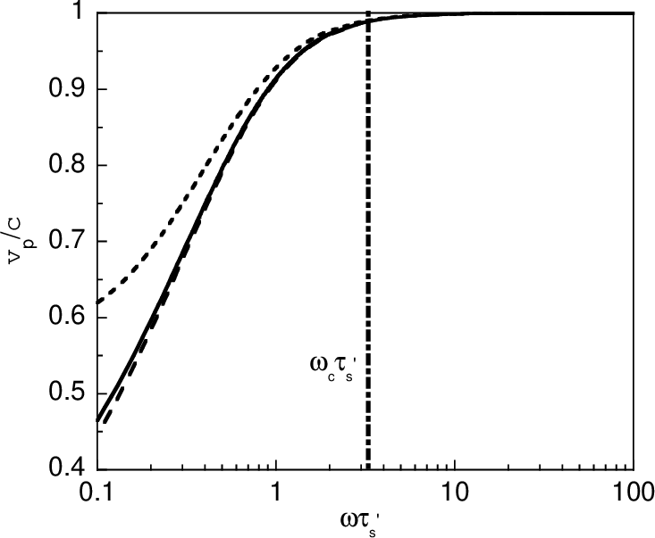
The phase velocity, defined as $v_{\mathrm{p}}=\omega/|k_{\mathrm{r}}|$, of the spin accumulation wave can be written as

When $\tilde{\omega}\rightarrow 0$ or $\infty$, the phase velocity $v_{\mathrm{p}}$ will approach $2c/(\eta^{1/2}+\eta^{-1/2})$ or $c$, respectively. When $\eta=1$, the phase velocity becomes equal to $c$ for all frequencies. Furthermore, the group velocity can be defined as $v_{\mathrm{g}}=d\omega/dk_{\mathrm{r}}$ and calculated from Eq. (26).

Figure 2 shows the phase velocity $v_{\mathrm{p}}$ as functions of $\tilde{\omega}$ for $\eta=0.1$, $0.02$, and $0.01$. The phase velocity is approximately equal to the wavefront velocity $c$ when the wave character is significant ($\omega>\omega_{\mathrm{c}}$). In this case, the phase velocity provides a good description of the wave-like dynamics. On the contrary, when the wave character is insignificant ($\omega<\omega_{\mathrm{c}}$), the wave amplitude is damped strongly and the phase velocity is not meaningful any more. In this region, the propagation velocity is the wavefront velocity $c$, albeit only on the length scale of a damping length.

In the special case where $\eta=1$ ($\tau^{\prime}_{s}=T_{1}$), we have $|k_{\mathrm{r}}|=w/c$ and $|k_{\mathrm{i}}|=1/l_{\mathrm{sf}}$. This means that the spin accumulation wave becomes a non-dispersive but dissipative wave with the constant phase (and group) velocity $c$ and penetration depth $l_{\mathrm{sf}}$. However, this case is likely not realized because $T_{1}$ is usually much larger than $\tau^{\prime}_{s}$ and Valet-Fert theory is justified to be valid only when $(\tau^{\prime}_{s}/2{T}_{1})^{1/2}\ll 1$.

In this section, the general analysis of the telegraph equations for spin-transport is augmented by numerical solutions for two illustrative examples of signal propagation using spin polarized currents through a ferromagnet/metal junction: (i) injection of an alternating current, and (ii) instantaneous magnetization switching. The results are obtained by numerically solving the system of Eqs. (10) and (11). Our numerical method is outlined in Appendix A.4. These equations are equivalent to the telegraph equations Eqs. (23) and (24), which have been discussed in the previous section, but are easier to solve. Alternatively, we could solve the equation system consisting of Eqs. (18) and (19), in which the spin accumulation is described by the spin density. However, it is more convenient to work with the electrochemical potential than the spin density when we deal with the boundary conditions.[19]

We choose a ferromagnet/metal junction consisting of Co and Cu as the material system in both of the scenarios. The interface of the junction is placed at $z=0$ and the Co (Cu) occupies the half-space $z>0$ ($z<0$). The positive direction of the current is parallel to the positive direction of the $z$ axis. For simplicity, the interface resistance of the junction will be neglected. Then, the electrochemical potential and the current density are continuous across the interface. Consequently, the spin transport across two layers can be described by one common equation system with different material parameters for the two layers.

The material parameters used in our numerical calculation are shown in Table 1. All other parameters can be obtained from the values in Tab. 1. In particular, the wavefront velocity is calculated to be $c=910$ nm/ps from Eq. (13). In the nonmagnetic layer, $\eta=\tau^{\prime}_{s}/T_{1}=0.02$. The wavelength $\lambda$ and damping length $l_{\mathrm{d}}$ are shown as the solid curves in Fig. 1. The critical period $T_{\mathrm{c}}$ can be estimated to be $2\tau^{\prime}_{s}\simeq 0.14$ ps from Eq. (31), and the phase velocity is plotted in Fig. 2.

We studied signal propagation in time-dependent spin transport through magnetic multilayers using an extension of the Valet-Fert theory to time-dependent phenomena. We established that time-dependent spin transport has a wave character in addition to its diffusive character, which enabled us to determine the finite propagation velocity of signals in spin transport, such as AC spin injection and magnetization switching. The propagation velocity is the wavefront velocity $c=v_{\mathrm{F}}/\sqrt{3}$. The wave character is significant if the signal time scale $\tau_{\mathrm{sig}}$ is smaller than a critical time $T_{\mathrm{c}}$. When the wave character is significant ($\tau_{\mathrm{sig}}<T_{\mathrm{c}}$), the time-dependent spin transport should be modeled by the dynamical equations introduced in this paper, or, equivalently, the telegraph equations. However, pure diffusive spin transport can be regarded as an approximation of the wave-diffusion duality for slow switching times ($\tau_{\mathrm{sig}}\gg{T}_{\mathrm{c}}$). In this limit, the spin diffusion equation can be used to study the time-dependence of spin transport approximately, but it incorrectly yields an infinite signal-propagation velocity.

References

- [1] I. Žutić, J. Fabian, and S. D. Sarma, Rev. Mod. Phys. 76, 323 (2004).
- [2] J. Fabian, A. Matos-Abiague, C. Ertler, P. Stano, and I. Žutić, Acta Phys. Slovaca 57, 565 (2007).
- [3] S. Zhang and P. M. Levy, Phys. Rev. B 65, 052409 (2002).
- [4] E. I. Rashba, Appl. Phys. Lett. 80, 2329 (2002).
- [5] J. Zhang and P. M. Levy, Phys. Rev. B 71, 184417 (2005).
- [6] Ł. Cywiński, H. Dery, and L. J. Sham, Appl. Phys. Lett. 89, 042105 (2006).
- [7] J. C. Maxwell, Phil. Trans. Roy. Soc. 157, 49 (1867).
- [8] G. Cattaneo, Atti. Sem. Mat. Fis. Univ. Modena 3, 83 (1948).
- [9] D. D. Joseph and L. Preziosi, Rev. Mod. Phys. 61, 41 (1989).
- [10] J. A. Scales and R. Snieder, Nature 401, 739 (1999).
- [11] T. Valet and A. Fert, Phys. Rev. B 48, 7099 (1993).
- [12] In general, the dynamical electric field is related to the scalar potential and vector potential by , However, if the magnetic field can be neglected for transport problems, one can find a gauge transformation that yields , cf.Refs. 3, 4, 5, 6.
- [13] A. Fert and S.-F. Lee, Phys. Rev. B 53, 6554 (1996).
- [14] M. Chester, Phys. Rev. 131, 2013 (1963).
- [15] A. M. Kadin, L. N. Smith, and W. J. Skocpol, J. Low Temp. Phys. 38, 497 (1980).
- [16] N. W. Ashcroft and N. D. Mermin, Solid State Physics (Brooks/Cole, Belmont, CA, 1976).
- [17] Q. Yang, P. Holody, S.-F. Lee, L. L. Henry, R. Loloee, P. A. Schroeder, J. W. P. Pratt, and J. Bass, Phys. Rev. Lett. 72, 3274 (1994).
- [18] L. Piraux, S. Dubois, A. Fert, and L. Belliard, Eur. Phys. J. B. 4, 413 (1998).
- [19] S. Hershfield and H. L. Zhao, Phys. Rev. B 56, 3296 (1997).
- [20] J. Masoliver and G. H. Weiss, Eur. J. Phys. 17, 190 (1996).
- [21] W. F. Ames, Numerical Methods for Partial Differential Equations (Academic Press, San Diego, California, 1992), 3rd ed., see Sec. 4-15.