跳到论文正文
W Papers独立论文阅读器 arXiv:0806.3833 论文正文 计算阅读时间 · 0%
引用这篇论文根据当前论文元数据生成,正式投稿前建议核对。


License: arXiv.org perpetual non-exclusive license
arXiv:0806.3833v1 [math.MG] 24 Jun 2008

Approximation of conformal mappings by circle patterns

Ulrike Bücking ††thanks: Partially supported by the DFG Research Unit “Polyhedral Surfaces” and by the DFG Research Center Matheon “Mathematics for key technologies”
Abstract

A circle pattern is a configuration of circles in the plane whose combinatorics is given by a planar graph GG such that to each vertex of GG there corresponds a circle. If two vertices are connected by an edge in GG then the corresponding circles intersect with an intersection angle in (0,π)(0,\pi) and these intersection points can be associated to the dual graph G∗G^{*}.

Two sequences of circle patterns are employed to approximate a given conformal map gg and its first derivative. For the domain of gg we use embedded circle patterns where all circles have the same radius εn>0\varepsilon_{n}>0 for a sequence εn→0\varepsilon_{n}\to 0 and where the intersection angles are uniformly bounded. The image circle patterns have the same combinatorics and intersection angles and are determined from boundary conditions (radii or angles) according to the values of g′g^{\prime} (|g′||g^{\prime}| or arg⁡g′\arg g^{\prime}). The error is of order 1/−log⁡εn1/\sqrt{-\log\varepsilon_{n}}. For quasicrystallic circle patterns the convergence result is strengthened to C∞C^{\infty}-convergence on compact subsets and an error of order εn\varepsilon_{n}.

1 Introduction

Conformal mappings constitute an important class in the field of complex analysis. They may be characterized by the fact that infinitesimal circles are mapped to infinitesimal circles. Suitable discrete analogs are of actual interest in the area of discrete differential geometry and its applications, see [BSSZ08].

Bill Thurston first introduced in his talk [Thu85] the idea to use finite circles, in particular circle packings, to define a discrete conformal mapping. Remember that an embedded planar circle packing is a configuration of closed disks with disjoint interiors in the plane ℂ\mathds{C}. Connecting the centers of touching disks by straight lines yields the tangency graph. Let 𝒞1{\mathscr{C}}_{1} and 𝒞2{\mathscr{C}}_{2} be two circle packings whose tangency graphs are combinatorially the same. Then there is a mapping g𝒞:𝒞1→𝒞2g_{\mathscr{C}}:{\mathscr{C}}_{1}\to{\mathscr{C}}_{2} which maps the centers of circles of 𝒞1{\mathscr{C}}_{1} to the corresponding centers of circles of 𝒞2{\mathscr{C}}_{2} and is an affine map on each triangular region corresponding to three mutually tangent circles. Various connections between circle packings and classical complex analysis have already been studied. A beautiful introduction and surway is presented by Stephenson in [Ste05]. In particular, several results concerning convergence, i.e. quantitative approximation of conformal mappings by g𝒞g_{\mathscr{C}}, have been obtained, see [RS87, CR92, HS96, HS98].

The class of circle patterns generalizes circle packings as for each circle packing there is an associated orthogonal circle pattern. Simply add a circle for each triangular face which passes through the three touching points. To define a circle pattern we use a planar graph as combinatorial data. The circles correspond to vertices and the edges specify which circles should intersect. The intersection angles are given using a labelling on the edges. Thus an edge corresponds to a kite of two intersecting circles as in Figure 1 (right). Moreover, for interior vertices the kites corresponding to the incident edges have disjoint interiors and their union is homeomorphic to a closed disk. Similarly as for circle packings, there are results on existence, rigidity, and construction of special circle pattern. See for example [Riv94, Sch97, AB00, BS04, BH03], where some of the references use a generalized notion of circle patterns.

Given two circle patterns 𝒞1{\mathscr{C}}_{1} and 𝒞2{\mathscr{C}}_{2} with the same combinatorics and intersection angles, define a mapping g𝒞:𝒞1→𝒞2g_{\mathscr{C}}:{\mathscr{C}}_{1}\to{\mathscr{C}}_{2} similarly as for circle packings. Namely, take g𝒞g_{\mathscr{C}} to map the centers of circles and the intersection points of 𝒞1{\mathscr{C}}_{1} corresponding to vertices and faces of GG to the corresponding centers of circles and intersection points of 𝒞2{\mathscr{C}}_{2} and extend it to an affine map on each kite.

For a given conformal map gg we use an analytic approach and specify suitable boundary values for the radius or the angle function according to |g′||g^{\prime}| or to arg⁡g′\arg g^{\prime} respectively in order to define the (approximating) mappings g𝒞g_{\mathscr{C}}. Generalizing ideas of Schramm’s convergence proof in [Sch97] we obtain convergence in C1C^{1} on compact sets if we take for 𝒞1(n){\mathscr{C}}_{1}^{(n)} a sequence of isoradial circle patterns (i.e. all radii are equal) with decreasing radii εn→0\varepsilon_{n}\to 0 which approximate the domain of gg. Furthermore, we assume that the intersection angles are uniformly bounded away from 00 and π\pi. Note in particular that the combinatorics of the circle pattern 𝒞1(n){\mathscr{C}}_{1}^{(n)} may be irregular or change within the sequence. Thus our convergence results applies to a considerably broader class of circle patterns as the known results of Schramm [Sch97], Matthes [Mat05], or Lan and Dai [LD07] for orthogonal circle patterns with square grid combinatorics.

The main idea of the proof is to consider a “nonlinear discrete Laplace equation” for the radius function. This equation turns out to be a (good) approximation of a known linear Laplace equation and can be used in the case of isoradial circle patterns to compare discrete and smooth solutions of the corresponding elliptic problems, that is the logarithm of the radii of 𝒞2(n){\mathscr{C}}_{2}^{(n)} and log⁡|g′|=Re​(log⁡g′)\log|g^{\prime}|=\text{Re}(\log g^{\prime}). Also, we obtain an a priori estimation of the approximation error of order 1/log⁡(1/εn)1/\sqrt{\log(1/\varepsilon_{n})}.

If the circle patterns 𝒞1(n){\mathscr{C}}_{1}^{(n)} additionally have only a uniformly bounded number of different edge directions, then the corresponding kite patterns are quasicrystallic rhombic embeddings and the circle patterns 𝒞1(n){\mathscr{C}}_{1}^{(n)} are called quasicrystallic [BMS05]. For such embeddings we generalize an asymptotic development given by Kenyon in [Ken02] of a discrete Green’s function. Also, using similar ideas as Duffin in [Duf53], we generalize theorems of discrete potential theory concerning the regularity of solutions of a discrete Laplace equation. We then use these results together with the C1C^{1}-convergence for isoradial circle patterns and prove C∞C^{\infty}-convergence on compact sets for a class of quasicrystallic circle patterns. In this case the approximation error is of order εn\varepsilon_{n} (or εn2\varepsilon_{n}^{2} for square grid or hexagonal combinatorics and regular intersection angles). The proof generalizes a method used by He and Schramm in [HS98].

The article is organized as follows: First we introduce and remind the terminology and some results on circle patterns in Section 2, focusing in particular on the radius and the angle function. In Section 3 we formulate and prove the theorems on C1C^{1}-convergence for isoradial circle patterns. After a brief review on quasicrystallic circle patterns in Section 4 we state and prove in Section 5 the theorem on C∞C^{\infty}-convergence. The necessary results on discrete potential theory are presented in Appendix A. An extended and more details version of the results can be found in [Büc07].

The author would like to thank Alexander I. Bobenko, Boris Springborn, and Yuri Suris for various discussions and helpful advice.

2 Circle patterns

To define circle patterns we use combinatorial data and intersection angles.

The combinatorics are specified by a b-quad-graph 𝒟\mathscr{D}, that is a strongly regular cell decomposition of a domain in ℂ\mathds{C} possibly with boundary such that all 2-cells (faces) are embedded and counterclockwise oriented. Furthermore all faces of 𝒟\mathscr{D} are quadrilaterals, that is there are exactly four edges incident to each face, and the 1-skeleton of 𝒟\mathscr{D} is a bipartite graph. We always assume that the vertices of 𝒟\mathscr{D} are colored white and black. To these two sets of vertices we associate two planar graphs GG and G∗G^{*} as follows. The vertices V⁡(G)V(G) are all white vertices of V⁡(𝒟)V(\mathscr{D}). The edges E⁡(G)E(G) correspond to faces of 𝒟\mathscr{D}, that is two vertices of GG are connected by an edge if and only if they are incident to the same face of 𝒟\mathscr{D}. The dual graph G∗G^{*} is constructed analogously by taking for V⁡(G∗)V(G^{*}) all black vertices of V⁡(𝒟)V(\mathscr{D}). 𝒟\mathscr{D} is called simply connected if it is the cell decomposition of a simply connected domain of ℂ\mathds{C} and if every closed chain of faces is null homotopic in 𝒟\mathscr{D}.

For the intersection angles, we use a labelling α:F⁡(𝒟)→(0,π)\alpha:F({\mathscr{D}})\to(0,\pi) of the faces of 𝒟\mathscr{D}. By abuse of notation, α\alpha can also be understood as a function defined on E⁡(G)E(G) or on E⁡(G∗)E(G^{*}). The labelling α\alpha is called admissible if it satisfies the following condition at all interior black vertices v∈Vi​n​t​(G∗)v\in V_{int}(G^{*}):

∑f​ incident to ​vα⁡(f)=2​π.\sum_{f\text{ incident to }v}\alpha(f)=2\pi. (1)
Refer to caption
α
Figure 1: Left: An example of a b-quad-graph 𝒟\mathscr{D} (black edges and bicolored vertices) and its associated graph GG (dashed edges and white vertices). Right: The exterior intersection angle α\alpha of two intersecting circles and the associated kite built from centers and intersection points.
Definition 2.1.

Let 𝒟\mathscr{D} be a b-quad-graph and let α:E⁡(G)→(0,π)\alpha:E(G)\to(0,\pi) be an admissible labelling. An (immersed planar) circle pattern for 𝒟\mathscr{D} (or GG) and α\alpha are an indexed collection 𝒞={Cz:z∈V⁡(G)}{\mathscr{C}}=\{C_{z}:z\in V(G)\} of circles in ℂ\mathds{C} and an indexed collection 𝒦={Ke:e∈E⁡(G)}={Kf:f∈F⁡(𝒟)}{\mathscr{K}}=\{K_{e}:e\in E(G)\}=\{K_{f}:f\in F({\mathscr{D}})\} of closed kites, which all carry the same orientation, such that the following conditions hold.

  1. (1)

    If z1,z2∈V⁡(G)z_{1},z_{2}\in V(G) are incident vertices in GG, the corresponding circles Cz1,Cz2C_{z_{1}},C_{z_{2}} intersect with exterior intersection angle α⁡([z1,z2])\alpha([z_{1},z_{2}]). Furthermore, the kite K[z1,z2]K_{[z_{1},z_{2}]} is bounded by the centers of the circles Cz1,Cz2C_{z_{1}},C_{z_{2}}, the two intersection points, and the corresponding edges, as in Figure 1 (right). The intersection points are associated to black vertices of V⁡(𝒟)V(\mathscr{D}) or to vertices of V⁡(G∗)V(G^{*}).

  2. (2)

    If two faces are incident in 𝒟\mathscr{D}, then the corresponding kites have one edge in common.

  3. (3)

    Let f1,…,fn∈F⁡(𝒟)f_{1},\dots,f_{n}\in F({\mathscr{D}}) be the faces incident to an interior vertex v∈Vi​n​t​(𝒟)v\in V_{int}({\mathscr{D}}). Then the kites Kf1,…,KfnK_{f_{1}},\dots,K_{f_{n}} have mutually disjoint interiors. Their union Kf1∪⋯∪KfnK_{f_{1}}\cup\dots\cup K_{f_{n}} is homeomorphic to a closed disc and contains the point p⁡(v)p(v) corresponding to vv in its interior.

The circle pattern is called embedded if all kites of 𝒦\mathscr{K} have mutually disjoint interiors. It is called isoradial if all circles of 𝒞\mathscr{C} have the same radius.

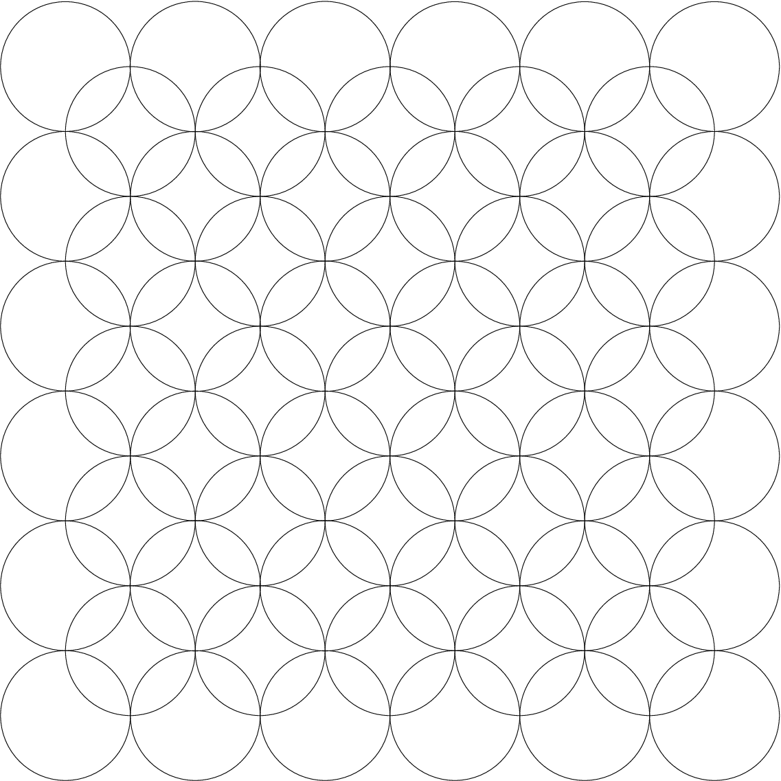
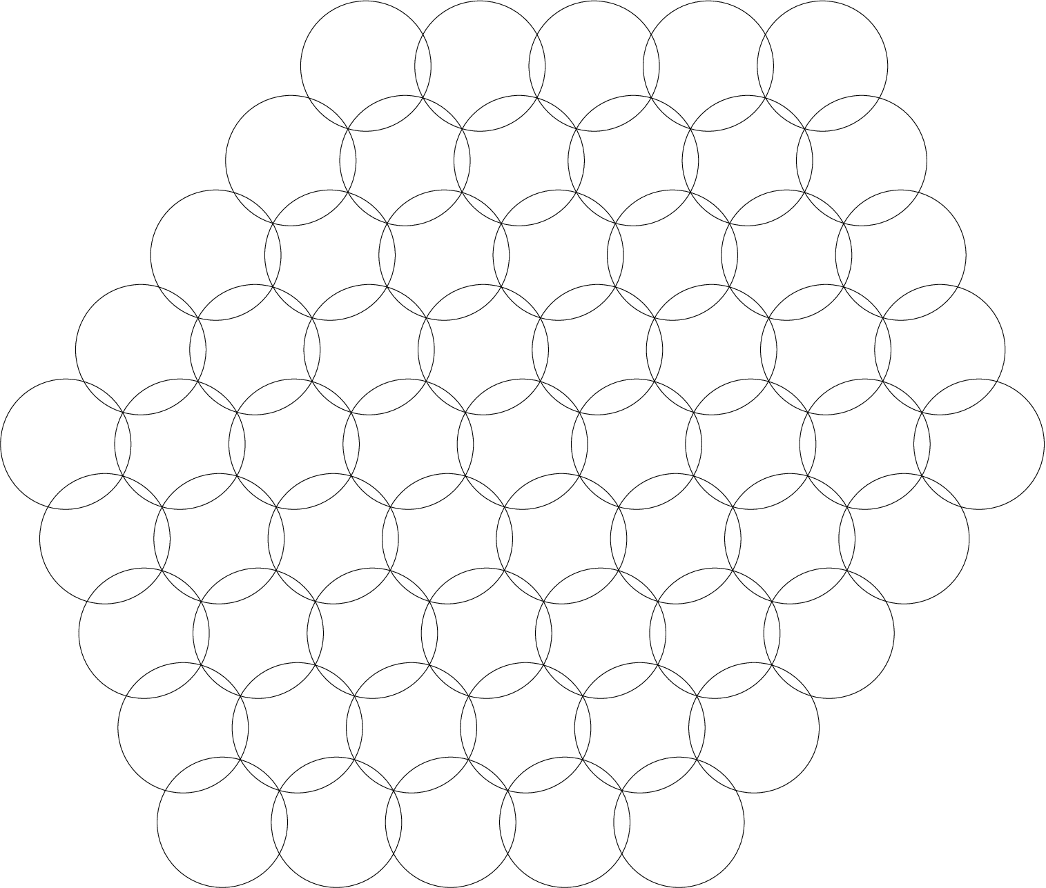
Note that we associate a circle pattern 𝒞\mathscr{C} to an immersion of the kite pattern 𝒦\mathscr{K} corresponding to 𝒟{\mathscr{D}} where the edges incident to the same white vertex are of equal length. The kites can also be reconstructed from the set of circles using the combinatorics of GG. Note further, that there are in general additional intersection points of circles which are not associated to black vertices of V⁡(𝒟)V({\mathscr{D}}). Some examples are shown in Figure 2.
Refer to caption
(a) A regular square grid circle pattern.
Refer to caption
(b) A regular hexagonal circle pattern.
Refer to caption
Refer to caption
(c) A rhombic embedding (a part of a Penrose tiling) and a corresponding isoradial circle pattern.
Figure 2: Examples of isoradial circle patterns.

There are also other definitions for circle patterns, for example associated to a Delaunay decomposition of a domain in ℂ\mathds{C}. This is a cell decomposition such that the boundary of each face is a polygon with straight edges which is inscribed in a circular disk, and these disks have no vertices in their interior. The corresponding circle pattern can be associated to the graph G∗G^{*}. The Poincaré-dual decomposition of a Delaunay decomposition with the centers of the circles as vertices and straight edges is a Dirichlet decomposition (or Voronoi diagram) and corresponds to the graph GG.

Furthermore the definition of circle patterns can be extended allowing cone-like singularities in the vertices; see [BS04] and the references therein.

2.1 The radius function

Our study of a planar circle pattern 𝒞{\mathscr{C}} is based on characterizations and properties of its radius function r𝒞=rr_{\mathscr{C}}=r which assigns to every vertex z∈V⁡(G)z\in V(G) the radius r𝒞​(z)=r​(z)r_{\mathscr{C}}(z)=r(z) of the corresponding circle CzC_{z}. The index 𝒞\mathscr{C} will be dropped whenever there is no confusion likely.

The following proposition specifies a necessary and sufficient condition for a radius function to originate from a planar circle pattern, see [BS04] for a proof. For the special case of orthogonal circle patterns with the combinatorics of the square grid, there are also other characterizations, see for example [Sch97].

Proposition 2.2.

Let GG be a graph constructed from a b-quad-graph 𝒟\mathscr{D} and let α\alpha be an admissible labelling.

Suppose that 𝒞{\mathscr{C}} is a planar circle pattern for 𝒟{\mathscr{D}} and α\alpha with radius function r=r𝒞r=r_{\mathscr{C}}. Then for every interior vertex z0∈Vi​n​t​(G)z_{0}\in V_{int}(G) we have

(∑[z,z0]∈E⁡(G)fα⁡([z,z0])​(log⁡r⁡(z)−log⁡r⁡(z0)))−π=0,\Biggl(\sum_{[z,z_{0}]\in E(G)}f_{\alpha([z,z_{0}])}(\log r(z)-\log r(z_{0}))\Biggr)-\pi=0, (2)

where

fθ​(x):=12​i​log⁡1−ex−i​θ1−ex+i​θ,f_{\theta}(x):=\frac{1}{2i}\log\frac{1-e^{x-i\theta}}{1-e^{x+i\theta}},

and the branch of the logarithm is chosen such that 0<fθ​(x)<π0<f_{\theta}(x)<\pi.

Conversely, suppose that 𝒟\mathscr{D} is simply connected and that r:V⁡(G)→(0,∞)r:V(G)\to(0,\infty) satisfies (2) for every z∈Vi​n​t​(G)z\in V_{int}(G). Then there is a planar circle pattern for GG and α\alpha whose radius function coincides with rr. This pattern is unique up to isometries of ℂ\mathds{C}.

Note that 2​fα⁡([z,z0])​(log⁡r⁡(z)−log⁡r⁡(z0))2f_{\alpha([z,z_{0}])}(\log r(z)-\log r(z_{0})) is the angle at z0z_{0} of the kite with edge lengths r⁡(z)r(z) and r⁡(z0)r(z_{0}) and angle α⁡([z,z0])\alpha([z,z_{0}]), as in Figure 1 (right). Equation (2) is the closing condition for the chain of kites corresponding to the edges incident to z0z_{0} which is condition (3) of Definition 2.1.

For further use we mention some properties of fθf_{\theta}, see for example [Spr03].

Lemma 2.3.
  1. (1)

    The derivative of fθf_{\theta} is fθ′​(x)=sin⁡θ2​(cosh⁡x−cos⁡θ)>0f_{\theta}^{\prime}(x)=\frac{\sin\theta}{2(\cosh x-\cos\theta)}>0. So fθf_{\theta} is strictly increasing.

  2. (2)

    The function fθf_{\theta} satisfies the functional equation fθ​(x)+fθ​(−x)=π−θf_{\theta}(x)+f_{\theta}(-x)=\pi-\theta.

  3. (3)

    For 0<y<π−θ0<y<\pi-\theta the inverse function of fθf_{\theta} is fθ−1​(y)=log⁡sin⁡ysin⁡(y+θ)f_{\theta}^{-1}(y)=\log\frac{\sin y}{\sin(y+\theta)}.

Remark 2.4.

Equation (2) can be interpreted as a nonlinear Laplace equation for the radius function and is related to a linear discrete Laplacian which is common in the linear theory of discrete holomorphic functions; see for example [Duf68, Mer01, BMS05] for more details. This can be seen as follows.

Let GG be a planar graph and let α\alpha be an admissible labelling. Assume there is a smooth one parameter family of planar circle patterns 𝒞ε{\mathscr{C}}_{\varepsilon} for GG and α\alpha with radius function rεr_{\varepsilon} for ε∈(−1,1)\varepsilon\in(-1,1). Then for every interior vertex z0z_{0} with incident vertices z1,…,zmz_{1},\dots,z_{m} and all ε∈(−1,1)\varepsilon\in(-1,1) Proposition 2.2 implies that

∑j=1m2​fα⁡([zj,z0])​(log⁡rε​(zj)−log⁡rε​(z0))=2​π.\sum_{j=1}^{m}2f_{\alpha([z_{j},z_{0}])}(\log r_{\varepsilon}(z_{j})-\log r_{\varepsilon}(z_{0}))=2\pi.

Differentiating this equation with respect to ε\varepsilon at ε=0\varepsilon=0, we obtain

∑j=1m2​fα⁡([zj,z0])′​(log⁡r0​(zj)−log⁡r0​(z0))​(v⁡(zj)−v⁡(z0))=0,\sum_{j=1}^{m}2f_{\alpha([z_{j},z_{0}])}^{\prime}(\log r_{0}(z_{j})-\log r_{0}(z_{0}))(v(z_{j})-v(z_{0}))=0, (3)

where v(z)=dd​εlogrε(z)|ε=0v(z)=\frac{d}{d\varepsilon}\log r_{\varepsilon}(z)\rvert_{\varepsilon=0}. Thus vv satisfies a linear discrete Laplace equation with positive weights. Lemma 2.3 and a simple calculation show that

2​fα⁡([z1,z2])′​(log⁡r0​(z1)−log⁡r0​(z2))=|p⁡(v1)−p⁡(v2)p⁡(z1)−p⁡(z2)|.2f_{\alpha([z_{1},z_{2}])}^{\prime}(\log r_{0}(z_{1})-\log r_{0}(z_{2}))=\left|\frac{p(v_{1})-p(v_{2})}{p(z_{1})-p(z_{2})}\right|. (4)

Here z1,z2∈V⁡(G)z_{1},z_{2}\in V(G) are two incident vertices which correspond to the centers of circles p⁡(z1),p⁡(z2)p(z_{1}),p(z_{2}) of the circle pattern 𝒞0{\mathscr{C}}_{0}. The two other corner points of the same kite are denoted by p⁡(v1),p⁡(v2)p(v_{1}),p(v_{2}).

In analogy to smooth harmonic functions, the radius function of a planar circle pattern satisfies a maximum principle and a Dirichlet principle.

Lemma 2.5 (Maximum Principle).

Let GG be a finite graph associated to a b-quad-graph as above with some admissible labelling α\alpha. Suppose 𝒞{\mathscr{C}} and 𝒞∗{\mathscr{C}}^{*} are two planar circle patterns for GG and α\alpha with radius functions r𝒞,r𝒞∗:V⁡(G)→(0,∞)r_{\mathscr{C}},r_{{\mathscr{C}}^{*}}:V(G)\to(0,\infty). Then the maximum and minimum of the quotient r𝒞/r𝒞∗r_{\mathscr{C}}/r_{{\mathscr{C}}^{*}} is attained at the boundary.

A proof can be found in [He99, Lemma 2.1]. If there exists an isoradial planar circle pattern for GG and α\alpha, the usual maximum principle for the radius function follows by taking r𝒞∗≡1r_{{\mathscr{C}}^{*}}\equiv 1.

Theorem 2.6 (Dirichlet Principle).

Let 𝒟\mathscr{D} be a finite simply connected b-quad-graph with associated graph GG and let α\alpha be an admissible labelling.

Let r:V∂​(G)→(0,∞)r:V_{\partial}(G)\to(0,\infty) be some positive function on the boundary vertices of GG. Then rr can be extended to V⁡(G)V(G) in such a way that equation (2) holds at every interior vertex z∈Vi​n​t​(G)z\in V_{int}(G) if and only if there exists any circle pattern for GG and α\alpha. If it exists, the extension is unique.

By lack of a good reference we include a proof.

Proof.

The only if part follows directly from the second part of Proposition 2.2.

To show the if part, assume that there exists a circle pattern for GG and α\alpha with radius function R:V⁡(G)→(0,∞)R:V(G)\to(0,\infty). A function κ:V⁡(G)→(0,∞)\kappa:V(G)\to(0,\infty) which satisfies the inequality

(∑[z,z0]∈E⁡(G)fα⁡([z,z0])​(log⁡κ⁡(z)−log⁡κ⁡(z0)))−π≥0\left(\sum_{[z,z_{0}]\in E(G)}f_{\alpha([z,z_{0}])}(\log\kappa(z)-\log\kappa(z_{0}))\right)-\pi\geq 0 (5)

at every interior vertex z∈Vi​n​t​(G)z\in V_{int}(G) will be called subharmonic in G. Let bb be the minimum of the quotient r/Rr/R on V∂​(G)V_{\partial}(G) and let κ1\kappa_{1} be equal to rr on V∂​(G)V_{\partial}(G) and to b​RbR on Vi​n​t​(G)V_{int}(G). Then κ1\kappa_{1} is clearly subharmonic. The maximum of κ1/R\kappa_{1}/R is attained at the boundary, which is a simple generalization of the Maximum Principle 2.5. Let r∗r^{*} be the supremum of all subharmonic functions on GG that coincide with rr on V∂​(G)V_{\partial}(G). Thus r∗r^{*} is bounded from above by the maximum of r/Rr/R on V∂​(G)V_{\partial}(G) which is finite. One easily checks that r∗r^{*} satisfies condition (2).

The uniqueness claim follows directly from the Maximum Principle 2.5. ∎

2.2 The angle function and relations to the radius function

Similarly as for polar coordinates of the complex plane, a suitably defined angle function can be interpreted as a “dual” to the radius function. We focus on connections between these functions and on a characterization for angle functions of circle patterns similar to Proposition 2.2.

Let GG be a finite graph associated to a b-quad-graph 𝒟\mathscr{D} and let α\alpha be an admissible labelling. Denote by E→​(𝒟)\vec{E}(\mathscr{D}) the set of oriented edges, where each edge of E⁡(𝒟)E(\mathscr{D}) is replaced by two oriented edges of opposite orientation. Let 𝒞{\mathscr{C}} be a planar circle pattern for 𝒟\mathscr{D} and α\alpha. Define an angle function φ𝒞=φ\varphi_{\mathscr{C}}=\varphi on E→​(𝒟)\vec{E}(\mathscr{D}) as follows. Denote by p⁡(w)p(w) the point of 𝒞\mathscr{C} corresponding to the vertex w∈V⁡(𝒟)w\in V(\mathscr{D}). For e→=z​v→∈E→​(𝒟)\vec{e}=\overrightarrow{zv}\in\vec{E}(\mathscr{D}) set φ⁡(e→)=arg⁡(p⁡(v)−p⁡(z))\varphi(\vec{e})=\arg(p(v)-p(z)) to be the argument of p⁡(v)−p⁡(z)p(v)-p(z), that is the angle between the positively oriented real axis and the vector p⁡(v)−p⁡(z)p(v)-p(z). As this argument is only unique up to addition of multiples of 2​π2\pi, we will mostly consider φ∈ℝ/(2​π​ℤ)\varphi\in\mathds{R}/(2\pi\mathds{Z}). But note that ei​φ​(e→)e^{i\varphi(\vec{e})} is well defined. Furthermore

φ⁡(e→)−φ⁡(−e→)=π(mod2​π).\varphi(\vec{e})-\varphi(-\vec{e})=\pi\pmod{2\pi}. (6)

Our choice of the angle function leads to the following connections between radius function rr and angle function φ\varphi for a planar circle pattern for 𝒟\mathscr{D} and α\alpha.

Let f∈F⁡(𝒟)f\in F({\mathscr{D}}) be a face of 𝒟{\mathscr{D}}. Without loss of generality, we assume that the notation for the vertices and edges of ff is taken from Figure 3 (left). More precisely, the white vertices z−z_{-} and z+z_{+} of ff and the black vertices v−v_{-} and v+v_{+} are labelled such that the points z−,v−,z+,v+z_{-},v_{-},z_{+},v_{+} appear in this cyclical order using the counterclockwise orientation of ff. Furthermore the edges are labelled such that e→1=z−​v+→\vec{e}_{1}=\overrightarrow{z_{-}v_{+}}, e→2=z−​v−→\vec{e}_{2}=\overrightarrow{z_{-}v_{-}}, −e→3=v−​z+→-\vec{e}_{3}=\overrightarrow{v_{-}z_{+}}, −e→4=v+​z+→-\vec{e}_{4}=\overrightarrow{v_{+}z_{+}}. Then the following equations hold.

φ⁡(e→1)−φ⁡(−e→3)\displaystyle\varphi(\vec{e}_{1})-\varphi(-\vec{e}_{3}) =α⁡(f)−π+2​fα⁡(f)​(log⁡r⁡(z+)−log⁡r⁡(z−))\displaystyle=\alpha(f)-\pi+2f_{\alpha(f)}(\log r(z_{+})-\log r(z_{-})) (mod2​π)\displaystyle\pmod{2\pi} (7)
φ⁡(−e→4)−φ⁡(e→2)\displaystyle\varphi(-\vec{e}_{4})-\varphi(\vec{e}_{2}) =α⁡(f)−π+2​fα⁡(f)​(log⁡r⁡(z+)−log⁡r⁡(z−))\displaystyle=\alpha(f)-\pi+2f_{\alpha(f)}(\log r(z_{+})-\log r(z_{-})) (mod2​π)\displaystyle\pmod{2\pi} (8)
φ⁡(e→1)−φ⁡(e→2)\displaystyle\varphi(\vec{e}_{1})-\varphi(\vec{e}_{2}) =2​fα⁡(f)​(log⁡r⁡(z+)−log⁡r⁡(z−))\displaystyle=2f_{\alpha(f)}(\log r(z_{+})-\log r(z_{-})) (mod2​π)\displaystyle\pmod{2\pi} (9)
φ⁡(−e→4)−φ⁡(−e→3)\displaystyle\varphi(-\vec{e}_{4})-\varphi(-\vec{e}_{3}) =−2​fα⁡(f)​(log⁡r⁡(z−)−log⁡r⁡(z+))\displaystyle=-2f_{\alpha(f)}(\log r(z_{-})-\log r(z_{+})) (mod2​π)\displaystyle\pmod{2\pi} (10)
φ⁡(−e→3)−φ⁡(e→2)\displaystyle\varphi(-\vec{e}_{3})-\varphi(\vec{e}_{2}) =π−α⁡(f)\displaystyle=\pi-\alpha(f) (mod2​π)\displaystyle\pmod{2\pi} (11)
φ⁡(−e→4)−φ⁡(e→1)\displaystyle\varphi(-\vec{e}_{4})-\varphi(\vec{e}_{1}) =α⁡(f)−π\displaystyle=\alpha(f)-\pi (mod2​π)\displaystyle\pmod{2\pi} (12)

Additionally, the angle function φ\varphi satisfies the following

Lemma 2.7 (Monotonicity condition).

Let z∈V⁡(G)z\in V(G) be a white vertex and let e1,…,ene_{1},\dots,e_{n} be the sequence of all incident edges in E⁡(𝒟)E(\mathscr{D}) which are cyclically ordered respecting the counterclockwise orientation of the circle CzC_{z}. Then the values of φ∈ℝ\varphi\in\mathds{R} can be changed by suitably adding multiples of 2​π2\pi such that φ⁡(e→j)\varphi(\vec{e}_{j}) is an increasing function of the index jj and if zz is an interior vertex, then also φ⁡(e→j)−φ⁡(e→1)<2​π\varphi(\vec{e}_{j})-\varphi(\vec{e}_{1})<2\pi for all j=1,…,nj=1,\dots,n.

α α β - β + z - z + v - v + → e 1 → e 2 - → e 4 - → e 3
α 1 α n ⁢ 2 β 1 r 2 ⁢ 2 β 2 r 1 ⁢ … …
Figure 3: Left: A face of 𝒟\mathscr{D} with oriented edges. Right: An interior intersection point with its neighboring faces.

The following theorem is useful to compare two circle patterns with the same combinatorics and intersection angles.

Theorem 2.8.

Let 𝒟\mathscr{D} be a b-quad-graph and let α\alpha be an admissible labelling.

Let 𝒞{\mathscr{C}} and 𝒞^\hat{\mathscr{C}} be two planar circle patterns for 𝒟\mathscr{D} and α\alpha with radius functions r𝒞=rr_{{\mathscr{C}}}=r and r𝒞^=r^r_{\hat{\mathscr{C}}}=\hat{r} and angle functions φ𝒞=φ\varphi_{\mathscr{C}}=\varphi and φ𝒞^=φ^\varphi_{\hat{\mathscr{C}}}=\hat{\varphi} respectively. Then the difference φ^−φ\hat{\varphi}-\varphi gives rise to a function δ:V⁡(G∗)→ℝ\delta:V(G^{*})\to\mathds{R} such that the following condition holds on every face f∈F⁡(𝒟)f\in F(\mathscr{D}).

2​fα⁡(f)​(log⁡(w⁡(z+)w⁡(z−))+log⁡(r⁡(z+)r⁡(z−)))−2​fα⁡(f)​(log⁡(r⁡(z+)r⁡(z−)))=δ⁡(v+)−δ⁡(v−)2f_{\alpha(f)}\left(\log\left({\textstyle\frac{w(z_{+})}{w(z_{-})}}\right)+\log\left({\textstyle\frac{r(z_{+})}{r(z_{-})}}\right)\right)-2f_{\alpha(f)}\left(\log\left({\textstyle\frac{r(z_{+})}{r(z_{-})}}\right)\right)=\delta(v_{+})-\delta(v_{-}) (13)

Here we have defined w:V⁡(G)→ℝw:V(G)\to\mathds{R}, w​(z)=r^​(z)/r​(z)w(z)=\hat{r}(z)/r(z) and the notation is taken from Figure 3 (left) as above.

Conversely, assume that 𝒞{\mathscr{C}} is a planar circle pattern for 𝒟\mathscr{D} and α\alpha with radius functions r𝒞=rr_{{\mathscr{C}}}=r and angle function φ𝒞=φ\varphi_{\mathscr{C}}=\varphi. Let δ:V⁡(G∗)→ℝ\delta:V(G^{*})\to\mathds{R} and w:V⁡(G)→ℝ+w:V(G)\to\mathds{R}_{+} be two functions which satisfy equation (13) for every face f∈F⁡(𝒟)f\in F(\mathscr{D}). Then (r​w)(rw) and (φ+δ)(\varphi+\delta) are the radius and angle function of a planar circle pattern for 𝒟\mathscr{D} and α\alpha. This circle pattern is unique up to translation.

Proof.

If 𝒞{\mathscr{C}} and 𝒞^\hat{\mathscr{C}} are two planar circle patterns for 𝒟\mathscr{D} and α\alpha, equations (6), (11), and (12) imply that the difference φ^−φ\hat{\varphi}-\varphi is constant for all edges incident to any fixed black vertex v∈V⁡(G∗)v\in V(G^{*}). Therefore δ(mod2​π)\delta\pmod{2\pi} is well defined on the intersection points and encodes the relative rotation of the star of edges at vv. Also equation (13) holds modulo 2​π2\pi.

To obtain a function δ\delta with values in ℝ\mathds{R}, fix δ⁡(v0)∈[0,2​π)\delta(v_{0})\in[0,2\pi) for one arbitrary vertex v0∈V⁡(G∗)v_{0}\in V(G^{*}) (for each connected component of G∗G^{*}). Define the values of δ\delta for all incident vertices in G∗G^{*} by equation (13). Continue this construction until a value has been assigned to all vertices. This proceedure leads to a well-defined function, as by Proposition 2.2 the sum of the left hand side of equation (13) is zero for simple closed paths in E⁡(G∗)E(G^{*}) around a white vertex.

To prove the converse claim, observe that if rr is a radius function, equation (13) implies that (w​r)(wr) fullfills equation (2). By Proposition 2.2 there is a circle pattern with radius function (w​r)(wr). Adjust the rotational freedom at one edge according to (φ+δ)(\varphi+\delta). Equation (13) implies that (φ+δ)(\varphi+\delta) is indeed the angle function of this circle pattern. ∎

The preceeding theorem motivates the definition of a comparison function for two circle patterns with the same combinatorics and intersection angles.

Let GG be a graph associated to a b-quad-graph 𝒟\mathscr{D} and let α\alpha be an admissible labelling. Suppose that 𝒞1{\mathscr{C}}_{1} and 𝒞2{\mathscr{C}}_{2} are planar circle patterns for 𝒟{\mathscr{D}} and α\alpha with radius functions r𝒞1r_{{\mathscr{C}}_{1}} and r𝒞2r_{{\mathscr{C}}_{2}} and angle functions φ𝒞1\varphi_{{\mathscr{C}}_{1}} and φ𝒞2\varphi_{{\mathscr{C}}_{2}} respectively. Let δ:V⁡(G∗)→ℝ\delta:V(G^{*})\to\mathds{R} be a function corresponding to φ𝒞2−φ𝒞1\varphi_{{\mathscr{C}}_{2}}-\varphi_{{\mathscr{C}}_{1}} as in Lemma 2.8. Define a comparison function w:V⁡(𝒟)→ℂw:V({\mathscr{D}})\to\mathds{C} by

{w⁡(y)=r𝒞2​(y)/r𝒞1​(y)for ​y∈V⁡(G),w⁡(x)=ei​δ​(x)∈𝕊1for ​x∈V⁡(G∗).\begin{cases}w(y)=r_{{\mathscr{C}}_{2}}(y)/r_{{\mathscr{C}}_{1}}(y)&\text{for }y\in V(G),\\ w(x)=\text{e}^{i\delta(x)}\in\mathds{S}^{1}&\text{for }x\in V(G^{*}).\end{cases} (14)

Note that w⁡(y)w(y) is the scaling factor of the circle corresponding to y∈V⁡(G)y\in V(G) when changing from the circle pattern 𝒞1{\mathscr{C}}_{1} to 𝒞2{\mathscr{C}}_{2}. w⁡(x)w(x) gives the rotation of the edge-star at x∈V⁡(G∗)x\in V(G^{*}). Furthermore, ww satisfies the following Hirota Equation for all faces f∈F⁡(𝒟)f\in F({\mathscr{D}}).

w⁡(x0)​w​(y0)​a0−w⁡(x1)​w​(y0)​a1−w⁡(x1)​w​(y1)​a0+w⁡(x0)​w​(y1)​a1=0w(x_{0})w(y_{0})a_{0}-w(x_{1})w(y_{0})a_{1}-w(x_{1})w(y_{1})a_{0}+w(x_{0})w(y_{1})a_{1}=0 (15)

Here x0,x1∈V⁡(G∗)x_{0},x_{1}\in V(G^{*}) and y0,y1∈V⁡(G)y_{0},y_{1}\in V(G) are the black and white vertices incident to ff and a0=x0−y0a_{0}=x_{0}-y_{0} and a1=x1−y0a_{1}=x_{1}-y_{0} are the directed edges. Equation (15) is the closing condition for the kite of 𝒞2{\mathscr{C}}_{2} which corresponds to the face ff.

Angle functions associated to planar circle patterns can be characterized in a similar way as radius functions are qualified in Proposition 2.2.

Proposition 2.9.

Let 𝒟\mathscr{D} be a b-quad-graph with associated graphs GG and G∗G^{*} and let α\alpha be an admissible labelling.

Suppose 𝒞{\mathscr{C}} is a planar circle pattern for 𝒟\mathscr{D} and α\alpha with angle function φ=φ𝒞\varphi=\varphi_{\mathscr{C}}. Then φ\varphi satisfies equations (6), (11), (12), the Monotonicity condition 2.7 at every white vertex of 𝒟\mathscr{D}, and the following two conditions.

  1. (i)

    Let ff be a face of 𝒟\mathscr{D} and let e1e_{1} and e2e_{2} be two edges incident to ff and to the same white vertex and assume that e1e_{1} and e2e_{2} are enumerated in clockwise order as in Figure 3 (left). Define an angle β∈(0,π)\beta\in(0,\pi) by

    2​β=φ⁡(e1→)−φ⁡(e2→)(mod2​π),2\beta=\varphi(\vec{e_{1}})-\varphi(\vec{e_{2}})\pmod{2\pi},

    where the orientation of the edges is chosen such that the vectors point from a white vertex to a black vertex, as in Figure 4 (left). Then

    β+α⁡(f)<π.\beta+\alpha(f)<\pi. (16)
  2. (ii)

    For an interior black vertex v∈Vi​n​t​(G∗)v\in V_{int}(G^{*}), denote by e1,…,en,en+1=e1e_{1},\dots,e_{n},e_{n+1}=e_{1} all incident edges of 𝒟\mathscr{D} in counterclockwise order and by fjf_{j} the face of 𝒟\mathscr{D} incident to eje_{j} and ej+1e_{j+1}. Denote by ej∗e_{j}^{*} (j=1,…,nj=1,\dots,n) the edge incident to eje_{j} and fjf_{j} which is not incident to vv. For j=1,…,nj=1,\dots,n define as above βj∈(0,π)\beta_{j}\in(0,\pi) by 2​βj=φ⁡(ej→)−φ⁡(ej→∗)(mod2​π)2\beta_{j}=\varphi(\vec{e_{j}})-\varphi(\vec{e_{j}}^{*})\pmod{2\pi}, where we choose the same orientation of the edges from white to black vertices as above. Then

    ∑j=1nfα⁡(fj)−1​(βj)=0.\displaystyle\sum_{j=1}^{n}f_{\alpha(f_{j})}^{-1}(\beta_{j})=0. (17)

Conversely, suppose that 𝒟\mathscr{D} is simply connected and that φ:E→​(𝒟)→ℝ/(2​π​ℤ)\varphi:\vec{E}({\mathscr{D}})\to\mathds{R}/(2\pi\mathds{Z}) satisfies equations (6), (11), (12), the Monotonicity condition 2.7, condition (16) at every white vertex of 𝒟\mathscr{D}, and condition (17) at every interior black vertex. Then there is a planar circle pattern for 𝒟\mathscr{D} and α\alpha with angle function φ\varphi. This pattern is unique up to scaling and translation.

Proof.

For a given planar circle pattern equations (7)–(12) and Lemma 2.7 hold. To show (16), consider a kite corresponding to a face of 𝒟\mathscr{D} as in Figure 3 (left). Note that β−=2​β\beta_{-}=2\beta by equation (9), β−+β++2​α=2​π\beta_{-}+\beta_{+}+2\alpha=2\pi, and β−,β+,α>0\beta_{-},\beta_{+},\alpha>0. Using notation of Figure 3 (right) we also deduce that fαj−1​(βj)=log⁡rj+1−log⁡rjf_{\alpha_{j}}^{-1}(\beta_{j})=\log r_{j+1}-\log r_{j} for j=1,…,nj=1,\dots,n, where we identify r1=rn+1r_{1}=r_{n+1}. Now (17) follows immediately.

In order to prove the converse claim, we construct a radius function r:V⁡(G)→(0,∞)r:V(G)\to(0,\infty) and build a circle pattern corresponding to rr and φ\varphi.

Let z∈V⁡(G)z\in V(G) be an interior white vertex. Set r⁡(z)=1r(z)=1. Consider a neighboring white vertex z′∈V⁡(G)z^{\prime}\in V(G) and the face f∈F⁡(𝒟)f\in F(\mathscr{D}) incident to zz and z′z^{\prime}. Denote the black vertices of 𝒟\mathscr{D} incident to zz and ff by v1v_{1}, v2v_{2} such that v1v_{1}, zz, v2v_{2}, z′z^{\prime} appear in counterclockwise order along the boundary of ff. Define ψ−∈(0,2​π)\psi_{-}\in(0,2\pi) by ψ−=φ⁡(z​v1→)−φ⁡(z​v2→)(mod2​π)\psi_{-}=\varphi(\overrightarrow{zv_{1}})-\varphi(\overrightarrow{zv_{2}})\pmod{2\pi}. Condition (16) implies that r⁡(z′):=r⁡(z)​exp​(fα⁡(f)−1​(ψ−/2))r(z^{\prime}):=r(z)\text{exp}(f_{\alpha(f)}^{-1}(\psi_{-}/2)) is well defined and positive. We proceed in this way until a radius has been assigned to all white vertices. Condition (17) guarantees that these assignments do not lead to different values when turning around a black vertex (see Figure 3 (right) with ψ=2​β\psi=2\beta). Thus rr is uniquely determined up to the choice of the initial radius, which corresponds to a global scaling. For each face f∈F⁡(𝒟)f\in F(\mathscr{D}) construct a kite with lengths r⁡(z+),r⁡(z−)r(z_{+}),r(z_{-}) of the edges incident to the white vertices z+,z−z_{+},z_{-} of ff respectively and angle α=α⁡(f)\alpha=\alpha(f). Lay out one kite fixing the rotational freedom according to φ\varphi. Successively add all other kites, respecting the combinatorics of 𝒟\mathscr{D}. By construction and assumptions, at every interior vertex the angles of the kites having this vertex in common add up to 2​π2\pi. Thus we obtain a circle pattern with angle function φ\varphi. ∎

3 C1C^{1}-convergence with Dirichlet or Neumann
boundary conditions

In this section we state and prove our main results on convergence for isoradial circle patterns. We begin with Dirichlet boundary conditions, that is we first focus on the radius function with given boundary values.

Theorem 3.1.

Let D⊂ℂD\subset\mathds{C} be a simply connected bounded domain, and let W⊂ℂW\subset\mathds{C} be open such that WW contains the closure D¯\overline{D} of DD. Let g:W→ℂg:W\to\mathds{C} be a locally injective holomorphic function. Assume, for convenience, that 0∈D0\in D.

For n∈ℕn\in\mathds{N} let 𝒟n{\mathscr{D}}_{n} be a b-quad-graph with associated graphs GnG_{n} and Gn∗G_{n}^{*} and let αn\alpha_{n} be an admissible labelling. We assume that 𝒟n{\mathscr{D}}_{n} is simply connected and that αn\alpha_{n} is uniformly bounded such that for all n∈ℕn\in\mathds{N} and all faces f∈F⁡(𝒟n)f\in F({\mathscr{D}}_{n})

|αn​(f)−π/2|<C|\alpha_{n}(f)-\pi/2|<C (18)

with some constant 0<C<π/20<C<\pi/2 independent of nn.

Let εn∈(0,∞)\varepsilon_{n}\in(0,\infty) be a sequence of positive numbers such that εn→0\varepsilon_{n}\to 0 for n→∞n\to\infty. For each n∈ℕn\in\mathds{N}, assume that there is an isoradial circle pattern for GnG_{n} and αn\alpha_{n}, where all circles have the same radius εn\varepsilon_{n}. Assume further that all centers of circles lie in the domain DD and that any point x∈D¯x\in\overline{D} which is not contained in any of the disks bounded by the circles of the pattern has a distance less than C^​εn\hat{C}\varepsilon_{n} to the nearest center of a circle and to the boundary ∂D\partial D, where C^>0\hat{C}>0 is some constant independent of nn. Denote by Rn≡εnR_{n}\equiv\varepsilon_{n} and ϕn\phi_{n} the radius and the angle function of the above circle pattern for GnG_{n} and αn\alpha_{n}. By abuse of notation, we do not distinguish between the realization of the circle pattern, that is the centers of circles znz_{n}, the intersection points vnv_{n}, and the edges connecting corresponding points in 𝒟n{\mathscr{D}}_{n} or GnG_{n}, and the abstract b-quad-graph 𝒟n{\mathscr{D}}_{n} and the graphs GnG_{n} and Gn∗G_{n}^{*}. Also, the index nn will be dropped from the notation of the vertices and the edges.

Define another radius function on GnG_{n} as follows. At boundary vertices z∈V∂​(Gn)z\in V_{\partial}(G_{n}) set

rn​(z)=Rn​(z)​|g′​(z)|.r_{n}(z)=R_{n}(z)\left|g^{\prime}(z)\right|. (19)

Using Theorem 2.6 extend rnr_{n} to a solution of the Dirichlet problem on GnG_{n}. Let z0∈V⁡(Gn)z_{0}\in V(G_{n}) be such that the disk bounded by the circle Cz0C_{z_{0}} contains 00 and let e=[z0,v0]∈E⁡(𝒟n)e=[z_{0},v_{0}]\in E({\mathscr{D}}_{n}) be one of the edges incident to z0z_{0} such that ϕn​(e→)∈[0,2​π)\phi_{n}(\vec{e})\in[0,2\pi) is minimal.

Let φn\varphi_{n} be the angle function corresponding to rnr_{n} that satisfies

φn​(e→)=arg⁡(g′​(v0))+ϕn​(e→).\varphi_{n}(\vec{e})=\arg\left(g^{\prime}(v_{0})\right)+\phi_{n}(\vec{e}). (20)

Let 𝒞n{\mathscr{C}}_{n} be the planar circle pattern with radius function rnr_{n} and angle function φn\varphi_{n}. Suppose that 𝒞n{\mathscr{C}}_{n} is normalized by a translation such that

pn​(v0)=g⁡(v0),p_{n}(v_{0})=g(v_{0}), (21)

where pn​(v)p_{n}(v) denotes the intersection point corresponding to v∈V⁡(Gn∗)v\in V(G_{n}^{*}). For z∈Dz\in D set

gn​(z)=pn​(w)andqn​(z)=rn​(v)Rn​(v)​ei⁡(φn​(v​w→)−ϕn​(v​w→)),g_{n}(z)=p_{n}(w)\hskip 10.00002pt\text{and}\hskip 10.00002ptq_{n}(z)=\frac{r_{n}(v)}{R_{n}(v)}e^{i(\varphi_{n}(\overrightarrow{vw})-\phi_{n}(\overrightarrow{vw}))},

where ww is a vertex of V⁡(Gn∗)V(G_{n}^{*}) closest to zz and vv is a vertex of V⁡(Gn)V(G_{n}) closest to zz such that [v,w]∈E⁡(𝒟n)[v,w]\in E({\mathscr{D}}_{n}).

Then qn→g′q_{n}\to g^{\prime} and gn→gg_{n}\to g uniformly on compact subsets in DD as n→∞n\to\infty.

Remark 3.2.

The proof of Theorem 3.1 actually shows the following a priori estimations for the approximating functions qnq_{n} and gng_{n}.

‖qn−g′‖V⁡(Gn)∩K≤C1​(−log2⁡εn)−12​ and ​‖gn−g‖V⁡(Gn)∩K≤C2​(−log2⁡εn)−12\|q_{n}-g^{\prime}\|_{V(G_{n})\cap K}\leq C_{1}(-\log_{2}\varepsilon_{n})^{-\frac{1}{2}}\ \text{ and }\ \|g_{n}-g\|_{V(G_{n})\cap K}\leq C_{2}(-\log_{2}\varepsilon_{n})^{-\frac{1}{2}}

for all compact sets K⊂DK\subset D, where the constants C1,C2C_{1},C_{2} depend on KK, gg, DD, and on the constants of Theorem 3.1.

We begin with an a priori estimation for the quotients of the radius functions.

Lemma 3.3.

For z∈V⁡(Gn)z\in V(G_{n}) set

hn​(z)=log⁡|g′​(z)|,\displaystyle h_{n}(z)=\log\left|g^{\prime}(z)\right|,
tn​(z)=log⁡(rn​(z)/Rn​(z))=log⁡(rn​(z)/εn).\displaystyle t_{n}(z)=\log(r_{n}(z)/R_{n}(z))=\log(r_{n}(z)/\varepsilon_{n}).

Then

hn​(z)−tn​(z)=𝒪⁡(εn).h_{n}(z)-t_{n}(z)={\cal O}(\varepsilon_{n}).

Here and below the notation s1=𝒪⁡(s2)s_{1}={\cal O}(s_{2}) means that there is a constant CC which may depend on W,D,gW,D,g, but not on nn and zz, such that |s1|≤C​s2|s_{1}|\leq Cs_{2} wherever s1s_{1} is defined. A direct consequence of Lemma 3.3 is

rn​(z)=Rn​(z)​|g′​(z)|+𝒪⁡(εn2).r_{n}(z)=R_{n}(z)\left|g^{\prime}(z)\right|+{\cal O}(\varepsilon_{n}^{2}). (22)

Our proof uses ideas of Schramm’s proof of the corresponding Lemma in [Sch97].

Proof.

Consider the function

p⁡(z)=tn​(z)−hn​(z)+β​|z|2,p(z)=t_{n}(z)-h_{n}(z)+\beta|z|^{2},

where β∈(0,1)\beta\in(0,1) is some function of εn\varepsilon_{n}. We want to choose β\beta such that pp will have no maximum in Vi​n​t​(Gn)V_{int}(G_{n}).

Suppose that pp has a maximum at z∈Vi​n​t​(Gn)z\in V_{int}(G_{n}). Denote by z1,…,zmz_{1},\dots,z_{m} the incident vertices of zz in GnG_{n} in counterclockwise order. Then we have

tn​(zj)−tn​(z)≤xjt_{n}(z_{j})-t_{n}(z)\leq x_{j} (23)

for j=1,…,mj=1,\dots,m where

xj=hn​(zj)−hn​(z)−β​|zj|2+β​|z|2.x_{j}=h_{n}(z_{j})-h_{n}(z)-\beta|z_{j}|^{2}+\beta|z|^{2}. (24)

Since z∈Vi​n​t​(Gn)z\in V_{int}(G_{n}), we have |z|=𝒪⁡(1)|z|={\cal O}(1) and by assumption z−zj=𝒪⁡(εn)z-z_{j}={\cal O}(\varepsilon_{n}). With β∈(0,1)\beta\in(0,1) this leads to β​|zj|2−β​|z|2=𝒪⁡(εn)\beta|z_{j}|^{2}-\beta|z|^{2}={\cal O}(\varepsilon_{n}). Using this estimate and the smoothness of Re​(log⁡g′)\text{Re}(\log g^{\prime}), we get xj=𝒪⁡(εn)x_{j}={\cal O}(\varepsilon_{n}).

From (23), the definition of tn​(z)=log⁡(rn​(z)/Rn​(z))=log⁡rn​(z)−log⁡εnt_{n}(z)=\log(r_{n}(z)/R_{n}(z))=\log r_{n}(z)-\log\varepsilon_{n} and the monotonicity of the sum in equation (2) (see Lemma 2.3 (i)), we get

0=(∑j=1mfα⁡(z,zj)​(log⁡rn​(zj)−log⁡rn​(z)⏟=tn​(zj)−tn​(z)))−π≤(∑j=1mfα⁡(z,zj)​(xj))−π.\displaystyle 0=\left(\sum_{j=1}^{m}f_{\alpha(z,z_{j})}(\underbrace{\log r_{n}(z_{j})-\log r_{n}(z)}_{=t_{n}(z_{j})-t_{n}(z)})\right)-\pi\leq\left(\sum_{j=1}^{m}f_{\alpha(z,z_{j})}\left(x_{j}\right)\right)-\pi. (25)

Remembering xj=𝒪⁡(εn)x_{j}={\cal O}(\varepsilon_{n}), we can consider a Taylor expansion of the right hand side of inequality (25) about 00 in order to make an 𝒪⁡(εn3){\cal O}(\varepsilon_{n}^{3})-analysis.

α j α j z z j v - j 1 v j a j a - j 1 a - j 1 a j
Figure 4: A rhombic face of 𝒟n{\mathscr{D}}_{n} with oriented edges.

Consider the chain of faces fjf_{j} of 𝒟n{\mathscr{D}}_{n} (j=1,…,mj=1,\dots,m) which are incident to zz and zjz_{j}. The enumeration of the vertices zjz_{j} (and hence of the faces fjf_{j}) and of the black vertices v1,…,vmv_{1},\dots,v_{m} incident to these faces can be chosen such that fjf_{j} is incident to vj−1v_{j-1} and vjv_{j} for j=1,…,mj=1,\dots,m, where v0=vmv_{0}=v_{m}. Furthermore, using this enumeration i⁡(zj−z)i(z_{j}-z) and (vj−vj−1)(v_{j}-v_{j-1}) are parallel, see Figure 4. As each face fjf_{j} of an isoradial circle pattern is a rhombus we can write, using the notation of Figure 4,

zj−z=aj−1+ajandvj−vj−1=aj−aj−1.\displaystyle z_{j}-z=a_{j-1}+a_{j}\hskip 20.00003pt\text{and}\hskip 20.00003ptv_{j}-v_{j-1}=a_{j}-a_{j-1}. (26)

Denoting αj=α⁡([z,zj])\alpha_{j}=\alpha([z,z_{j}]), lj=|zj−z|=2​εn​sin⁡(αj/2)l_{j}=|z_{j}-z|=2\varepsilon_{n}\sin(\alpha_{j}/2), and l^j=|vj−vj−1|=2​εn​cos⁡(αj/2)\hat{l}_{j}=|v_{j}-v_{j-1}|=2\varepsilon_{n}\cos(\alpha_{j}/2), we easily obtain by simple calculations that

fαj​(0)=(π−αj)/2,fαj′​(0)=l^j/(2​lj),fαj′′​(0)=0.\displaystyle f_{\alpha_{j}}(0)=(\pi-\alpha_{j})/2,\hskip 10.00002ptf_{\alpha_{j}}^{\prime}(0)=\hat{l}_{j}/(2l_{j}),\hskip 10.00002ptf_{\alpha_{j}}^{\prime\prime}(0)=0.

Taking into account that equation (2) holds with Rn≡εnR_{n}\equiv\varepsilon_{n} and using the uniform boundedness (18) of the labelling α\alpha, inequality (25) yields

0≤∑j=1mfαj′​(0)​xj+𝒪⁡(εn3).0\leq\sum_{j=1}^{m}f_{\alpha_{j}}^{\prime}(0)x_{j}+{\cal O}(\varepsilon_{n}^{3}). (27)

To evaluate this sum, expand

hn​(zj)−hn​(z)=Re​(log⁡g′​(zj)−log⁡g′​(z))=Re​(a⁡(zj−z)+b​(zj−z)2)+𝒪⁡(εn3)\displaystyle h_{n}(z_{j})-h_{n}(z)=\text{Re}(\log g^{\prime}(z_{j})-\log g^{\prime}(z))=\text{Re}(a(z_{j}-z)+b(z_{j}-z)^{2})+{\cal O}(\varepsilon_{n}^{3})
and ​xj=hn​(zj)−hn​(z)−β​|zj|2+β​|z|2=Re​(a⁡(zj−z)+b​(zj−z)2−2​β​z¯​(zj−z))−β​lj2+𝒪⁡(εn3).\displaystyle\begin{split}\text{and }\ x_{j}&=h_{n}(z_{j})-h_{n}(z)-\beta|z_{j}|^{2}+\beta|z|^{2}\\ &=\text{Re}(a(z_{j}-z)+b(z_{j}-z)^{2}-2\beta\bar{z}(z_{j}-z))-\beta l_{j}^{2}+{\cal O}(\varepsilon_{n}^{3}).\end{split}

Noting that fαj′​(0)​(zj−z)=(vj−vj−1)/(2​i)f_{\alpha_{j}}^{\prime}(0)(z_{j}-z)=(v_{j}-v_{j-1})/(2i) we get

∑j=1mfαj′​(0)​xj\displaystyle\sum_{j=1}^{m}f_{\alpha_{j}}^{\prime}(0)x_{j} =Re​(a−2​β​z¯2​i​∑j=1m(vj−vj−1)⏟=0+b2​i​∑j=1m(vj−vj−1)​(zj−z)⏟=(26)(aj−aj−1)​(aj+aj−1)⏟=0)\displaystyle=\text{Re}\Biggl(\frac{a-2\beta\bar{z}}{2i}\underbrace{\sum_{j=1}^{m}(v_{j}-v_{j-1})}_{=0}+\frac{b}{2i}\underbrace{\sum_{j=1}^{m}\underbrace{(v_{j}-v_{j-1})(z_{j}-z)}_{\stackrel{{\scriptstyle\eqref{eqzva}}}{{=}}(a_{j}-a_{j-1})(a_{j}+a_{j-1})}}_{=0}\Biggr)
−β∑j=1mlj​l^j2+𝒪(εn3).\displaystyle\,\hskip 10.00002pt-\beta\sum_{j=1}^{m}\frac{l_{j}\hat{l}_{j}}{2}+{\cal O}(\varepsilon_{n}^{3}).

Thus from inequality (27), remembering lj=2​εn​sin⁡(αj/2)l_{j}=2\varepsilon_{n}\sin(\alpha_{j}/2) and l^j=2​εn​cos⁡(αj/2)\hat{l}_{j}=2\varepsilon_{n}\cos(\alpha_{j}/2), we arrive at

0≤−βεn2∑j=1msin(αj/2)cos(αj/2)+𝒪(εn3)⇔β∑j=1msin(αj)≤𝒪(εn).0\leq-\beta\varepsilon_{n}^{2}\sum_{j=1}^{m}\sin(\alpha_{j}/2)\cos(\alpha_{j}/2)+{\cal O}(\varepsilon_{n}^{3})\hskip 10.00002pt\iff\hskip 10.00002pt\beta\sum_{j=1}^{m}\sin(\alpha_{j})\leq{\cal O}(\varepsilon_{n}).

Note that εn2​∑j=1msin⁡(αj)>π​εn2\varepsilon_{n}^{2}\sum_{j=1}^{m}\sin(\alpha_{j})>\pi\varepsilon_{n}^{2} is the area of the rhombic faces incident to the vertex zz. Thus we conclude that β=𝒪⁡(εn)\beta={\cal O}(\varepsilon_{n}). This means, that if we choose β=C​εn\beta=C\varepsilon_{n} with C>0C>0 a sufficiently large constant and if εn\varepsilon_{n} is small enough such that C​εn<1C\varepsilon_{n}<1, then pp will have no maximum in Vi​n​t​(Gn)V_{int}(G_{n}). In that case, as we have p⁡(z)=β​|z|2=𝒪⁡(εn)p(z)=\beta|z|^{2}={\cal O}(\varepsilon_{n}) on V∂​(Gn)V_{\partial}(G_{n}), we deduce that p⁡(z)≤𝒪⁡(εn)p(z)\leq{\cal O}(\varepsilon_{n}) in V⁡(Gn)V(G_{n}) and thus

tn​(z)−hn​(z)≤𝒪⁡(εn)for ​z∈V⁡(Gn).t_{n}(z)-h_{n}(z)\leq{\cal O}(\varepsilon_{n})\hskip 20.00003pt\text{for }z\in V(G_{n}). (28)

The proof for the reverse inequality is almost the same. The only modifications needed are reversing the sign of β\beta and a few inequalities. ∎

Remark 3.4.

The statement of Lemma 3.3 can be improved to

hn​(z)−tn​(z)=𝒪⁡(εn2)h_{n}(z)-t_{n}(z)={\cal O}(\varepsilon_{n}^{2}) (29)

in the case of a ’very regular’ isoradial circle pattern. These are isoradial circle patterns such that for every oriented edge ej1=zj1−z∈E→​(G)e_{j_{1}}=z_{j_{1}}-z\in\vec{E}(G) incident to an interior vertex z∈Vi​n​t​(G)z\in V_{int}(G) there is another parallel edge ej2=zj2−z∈E→​(G)e_{j_{2}}=z_{j_{2}}-z\in\vec{E}(G) with opposite direction incident to zz, that is ej2=−ej1e_{j_{2}}=-e_{j_{1}}. Furthermore, the corresponding intersection angles agree: α⁡([z,zj1])=α⁡([z,zj2])\alpha([z,z_{j_{1}}])=\alpha([z,z_{j_{2}}]). This additional regularity property holds for example for an orthogonal circle pattern with the combinatorics of a part of the square grid, see Figure 2(a).

The proof of estimation (29) follows the same reasonings as above, but makes an 𝒪⁡(εn4){\cal O}(\varepsilon_{n}^{4})-analysis. The additional regularity implies that all terms of order εn3\varepsilon_{n}^{3} vanish.

Definition 3.5.

For a function η:V⁡(G)→ℝ\eta:V(G)\to\mathds{R} define a discrete Laplacian by

Δ​η​(z)=∑[z,zj]∈E⁡(G)2​fα⁡([z,zj])′​(0)​(η⁡(zj)−η⁡(z)).\Delta\eta(z)=\sum_{[z,z_{j}]\in E(G)}2f^{\prime}_{\alpha([z,z_{j}])}(0)(\eta(z_{j})-\eta(z)). (30)

As fα⁡([z1,z2])′​(0)>0f^{\prime}_{\alpha([z_{1},z_{2}])}(0)>0 one immediately has the following

Lemma 3.6 (Maximum Principle).

If Δ​η≥0\Delta\eta\geq 0 on Vi​n​t​(G)V_{int}(G) then the maximum of η\eta is attained at the boundary V∂​(G)V_{\partial}(G).

The proof of Lemma 3.3 actually shows, that tn−hnt_{n}-h_{n} is almost harmonic. More precisely, we have Δ⁡(tn−hn)=𝒪⁡(εn3)\Delta(t_{n}-h_{n})={\cal O}(\varepsilon_{n}^{3}). Adding a suitable subharmonic function β​|z|2\beta|z|^{2} with β>0\beta>0 big enough, we deduce that the resulting function pp is subharmonic, that is Δ​p≥0\Delta p\geq 0, such that pp attains its maximum at the boundary. This is also important for our proof of the following lemma.

Lemma 3.7.

Let tnt_{n} and hnh_{n} be defined as in Lemma 3.3. Let K⊂DK\subset D be a compact subset in DD. Then the following estimation holds for every interior vertex z∈Vi​n​t​(Gn)∩Kz\in V_{int}(G_{n})\cap K such that all its incident vertices z1,…,zlz_{1},\dots,z_{l} are also in Vi​n​t​(Gn)∩KV_{int}(G_{n})\cap K:

tn​(zj)−hn​(zj)−(tn​(z)−hn​(z))=𝒪⁡(εn​(−log⁡εn)−12).t_{n}(z_{j})-h_{n}(z_{j})-(t_{n}(z)-h_{n}(z))={\cal O}(\varepsilon_{n}(-\log\varepsilon_{n})^{-\frac{1}{2}}). (31)

for j=1,…,lj=1,\dots,l. The constant in the 𝒪{\cal O}-notation may depend on KK, but not on nn or zz.

The proof of Lemma 3.7 uses the following estimation for superharmonic functions, which is a version of Corollary 3.1 of [SC97]; see also [SC97, Remark 3.2 and Lemma 2.1].

Proposition 3.8 ([SC97]).

Let GG be an undirected connected graph without loops and let c:E⁡(G)→ℝ+c:E(G)\to\mathds{R}^{+} be a positive weight function on the edges. Denote c⁡(e)=c⁡(x,y)c(e)=c(x,y) for an edge e=[x,y]∈E⁡(G)e=[x,y]\in E(G) and assume that

m=max⁡∑[x,z]∈E⁡(G)[x,y]∈E⁡(G)⁡c⁡(x,z)c⁡(x,y)<∞.m=\max_{[x,y]\in E(G)}\sum_{[x,z]\in E(G)}\frac{c(x,z)}{c(x,y)}<\infty.

Denote by d⁡(x,y)d(x,y) the combinatorial distance between two vertices x,y∈V⁡(G)x,y\in V(G) in the graph GG. Let Bx​(ϱ)={y∈V⁡(G):d⁡(x,y)≤ϱ}B_{x}(\varrho)=\{y\in V(G):d(x,y)\leq\varrho\} be the combinatorial ball of radius ϱ>0\varrho>0 around the vertex x∈V⁡(G)x\in V(G). Fix x∈V⁡(G)x\in V(G) and R≥4R\geq 4 and set

AR=sup1≤ϱ≤Rϱ−2​Wx​(ϱ),whereWx​(ϱ)=∑z∈Bx​(ϱ),y∈V⁡(G)d⁡(x,z)<d⁡(x,y)c⁡(z,y).A_{R}=\sup_{1\leq\varrho\leq R}\varrho^{-2}W_{x}(\varrho),\hskip 20.00003pt\text{where}\hskip 20.00003ptW_{x}(\varrho)=\sum_{\begin{subarray}{c}z\in B_{x}(\varrho),\ y\in V(G)\\ d(x,z)<d(x,y)\end{subarray}}c(z,y).

Let uu be a positive superharmonic function in Bx​(R+1)B_{x}(R+1), that is

∑[z,w]∈E⁡(G)c⁡(z,w)​(u⁡(z)−u⁡(w))≤0\sum_{[z,w]\in E(G)}c(z,w)(u(z)-u(w))\leq 0

for all w∈Bx​(R+1)w\in B_{x}(R+1). Let yy be incident to xx in GG. Then

|u⁡(x)u⁡(y)−1|≤4​m2​ARc⁡(x,y)​log2​R.\left|\frac{u(x)}{u(y)}-1\right|\leq\frac{4m^{2}\sqrt{A_{R}}}{\sqrt{c(x,y)\log_{2}R}}.
Proof of Lemma 3.7.

Lemma 3.3 implies that tn​(zj)−tn​(z)=𝒪⁡(εn)t_{n}(z_{j})-t_{n}(z)={\cal O}(\varepsilon_{n}) for all incident vertices z,zj∈V⁡(Gn)z,z_{j}\in V(G_{n}) since hn=log⁡|g′|h_{n}=\log|g^{\prime}| is a C∞C^{\infty}-function. Consider a Taylor expansion about 00 of

0=(∑j=1mfα⁡(z,zj)​(tn​(zj)−tn​(z)))−π.0=\Biggl(\sum_{j=1}^{m}f_{\alpha(z,z_{j})}(t_{n}(z_{j})-t_{n}(z))\Biggr)-\pi.

Similar reasonings as in the proof of Lemma 3.3 imply that Δ​tn​(z)=𝒪⁡(εn3)\Delta t_{n}(z)={\cal O}(\varepsilon_{n}^{3}). Let p=tn−hn+β​|z|2p=t_{n}-h_{n}+\beta|z|^{2} with β∈(0,1)\beta\in(0,1). Choosing β=C​εn\beta=C\varepsilon_{n} with a sufficiently large constant C>0C>0 and εn\varepsilon_{n} small enough we deduce similarly as in the proof of Lemma 3.3 that Δ​p​(z)≥0\Delta p(z)\geq 0 for all interior vertices z∈Vi​n​t​(Gn)z\in V_{int}(G_{n}). Now define the positive function p^=εn+‖p‖−p\hat{p}=\varepsilon_{n}+\|p\|-p. Then Δ​p^​(z)≤0\Delta\hat{p}(z)\leq 0 for all z∈Vi​n​t​(Gn)z\in V_{int}(G_{n}). The proof of Lemma 3.3 shows that there is a constant C1C_{1}, depending only on gg, DD, and the labelling α\alpha, such that ‖p‖≤C1​εn\|p\|\leq C_{1}\varepsilon_{n}. Thus ‖p^‖≤C2​εn\|\hat{p}\|\leq C_{2}\varepsilon_{n} with C2=2​C1+1C_{2}=2C_{1}+1.

To finish to proof, we apply Proposition 3.8 to the superharmonic function p^\hat{p}. Remember that GnG_{n} is a connected graph without loops and c⁡(e):=2​fα⁡(e)′​(0)>0c(e):=2f_{\alpha(e)}^{\prime}(0)>0 defines a positive weight function on the edges. The bound (18) on the labelling α\alpha implies that

m=max⁡∑[x,z]∈E⁡(Gn)[x,y]∈E⁡(Gn)⁡c⁡(x,z)c⁡(x,y)<2​ππ/2−C​cot⁡(π/4−C/2)cot⁡(π/4+C/2)=:C3<∞.m=\max_{[x,y]\in E(G_{n})}\sum_{[x,z]\in E(G_{n})}\frac{c(x,z)}{c(x,y)}<\frac{2\pi}{\pi/2-C}\frac{\cot(\pi/4-C/2)}{\cot(\pi/4+C/2)}=:C_{3}<\infty.

Let x∈Vi​n​t​(Gn)x\in V_{int}(G_{n}). Note that

Wx​(ϱ)=∑z∈Bx​(ϱ),y∈V⁡(Gn)d⁡(x,z)<d⁡(x,y)c⁡(z,y)≤(maxe∈E⁡(Gn)⁡c⁡(e))​|Fw​(x,ϱ)|,W_{x}(\varrho)=\sum_{\begin{subarray}{c}z\in B_{x}(\varrho),\;y\in V(G_{n})\\ d(x,z)<d(x,y)\end{subarray}}c(z,y)\leq\left(\max_{e\in E(G_{n})}c(e)\right)|F_{w}(x,\varrho)|,

where Fw​(x,ϱ)F_{w}(x,\varrho) is the set of all faces of 𝒟n{\mathscr{D}}_{n} with one white vertex z∈Bx​(ϱ)z\in B_{x}(\varrho) and |Fw​(x,ϱ)||F_{w}(x,\varrho)| denotes the number of faces of Fw​(x,ϱ)F_{w}(x,\varrho). Now, maxe∈E⁡(Gn)⁡c⁡(e)<cot⁡(π/4−C/2)/2\max_{e\in E(G_{n})}c(e)<\cot(\pi/4-C/2)/2 and

Fw​(x,ϱ)⊂Dx​((ϱ+1)​2​εn)={w∈ℂ:|w−x|≤(ϱ+1)​2​εn},F_{w}(x,\varrho)\subset D_{x}((\varrho+1)2\varepsilon_{n})=\{w\in\mathds{C}:|w-x|\leq(\varrho+1)2\varepsilon_{n}\},

as the edge lengths in GnG_{n} are smaller than 2​εn2\varepsilon_{n}. Remember that F⁡(f)=εn2​sin⁡α⁡(f)>εn2​sin⁡(π/2−C)F(f)=\varepsilon_{n}^{2}\sin\alpha(f)>\varepsilon_{n}^{2}\sin(\pi/2-C) is the area of the face f∈F⁡(𝒟n)f\in F({\mathscr{D}}_{n}). Thus

|Fw​(x,ϱ)|<π​((ϱ+1)​2​εn)2εn2​sin⁡(π/2−C)≤16​π​ϱ2sin⁡(π/2−C)=:ϱ2​C4|F_{w}(x,\varrho)|<\frac{\pi((\varrho+1)2\varepsilon_{n})^{2}}{\varepsilon_{n}^{2}\sin(\pi/2-C)}\leq\frac{16\pi\varrho^{2}}{\sin(\pi/2-C)}=:\varrho^{2}C_{4}

for all ϱ≥1\varrho\geq 1. Therefore we obtain AR=sup1≤ϱ≤Rϱ−2​Wx​(ϱ)<C4A_{R}=\sup_{1\leq\varrho\leq R}\varrho^{-2}W_{x}(\varrho)<C_{4}, where the upper bound C4C_{4} is independent of R≥4R\geq 4 and n∈ℕn\in\mathds{N}.

Let K⊂DK\subset D be compact. Denote by 𝕖\mathbb{e} the Euclidean distance (between a point and a compact set or between closed sets of ℝ2≅ℂ\mathds{R}^{2}\cong\mathds{C}). Let z∈V⁡(Gn)∩Kz\in V(G_{n})\cap K and set (R+1)=d⁡(z,V∂​(Gn))(R+1)=d(z,V_{\partial}(G_{n})) to be the combinatorial distance from zz to the boundary of GnG_{n}. Let zj∈V⁡(Gn)z_{j}\in V(G_{n}) be incident to zz. As the labelling α\alpha is bounded, εn→0\varepsilon_{n}\to 0, and 𝒟n{\mathscr{D}}_{n} approximates DD, we deduce that R≥εn−1​C5≥4R\geq\varepsilon_{n}^{-1}C_{5}\geq 4 if n≥n0n\geq n_{0} is large enough. Thus for all n≥n0n\geq n_{0} and all z∈V⁡(Gn)∩Kz\in V(G_{n})\cap K

1/log2⁡R≤1/log2⁡C5−log2⁡εn≤2/−log2⁡εn1/\sqrt{\log_{2}R}\leq 1/\sqrt{\log_{2}C_{5}-\log_{2}\varepsilon_{n}}\leq\sqrt{2}/\sqrt{-\log_{2}\varepsilon_{n}}

holds by our assumptions. Proposition 3.8 implies that

|p^​(z)p^​(zj)−1|≤4​C32​C4​2−c⁡(z,zj)​log2​εn\left|\frac{\hat{p}(z)}{\hat{p}(z_{j})}-1\right|\leq\frac{4C_{3}^{2}\sqrt{C_{4}}\sqrt{2}}{\sqrt{-c(z,z_{j})\log_{2}\varepsilon_{n}}}

for all incident vertices z,zj∈V⁡(Gn)∩Kz,z_{j}\in V(G_{n})\cap K and n≥n0n\geq n_{0}. As c⁡(z,zj)≤cot⁡(π/4−C/2)/2c(z,z_{j})\leq\cot(\pi/4-C/2)/2 and ‖p^‖≤C2​εn\|\hat{p}\|\leq C_{2}\varepsilon_{n} we finally arrive at the desired estimation

|tn​(zj)−hn​(zj)−(tn​(z)−hn​(z))|=|p^​(z)−p^​(zj)|≤C6​εn​(−log2⁡εn)−12|t_{n}(z_{j})-h_{n}(z_{j})-(t_{n}(z)-h_{n}(z))|=|\hat{p}(z)-\hat{p}(z_{j})|\leq C_{6}\varepsilon_{n}(-\log_{2}\varepsilon_{n})^{-\frac{1}{2}}

for all incident vertices z,zj∈V⁡(Gn)∩Kz,z_{j}\in V(G_{n})\cap K and n≥n0n\geq n_{0}, where the constant C6C_{6} depends on C2,…,C5C_{2},\dots,C_{5}, that is only on gg, DD, CC, C^\hat{C}, and KK. ∎

Lemma 3.9.

Let e→=u​v→∈E→​(𝒟n)\vec{e}=\overrightarrow{uv}\in\vec{E}({\mathscr{D}}_{n}) be a directed edge with u∈V⁡(Gn)u\in V(G_{n}) and v∈V⁡(Gn∗)v\in V(G_{n}^{*}). Denote by δn​(e)\delta_{n}({e}) the combinatorial distance in 𝒟n{\mathscr{D}}_{n} from e=[u,v]e=[u,v] to [z0,v0][z_{0},v_{0}], that is the least integer kk such that there is a sequence of edges {[z0,v0]=e1,e2,…,ek=e}⊂E⁡(𝒟n)\{[z_{0},v_{0}]=e_{1},e_{2},\dots,e_{k}=e\}\subset E({\mathscr{D}}_{n}) such that the edges em+1e_{m+1} and eme_{m} are incident to the same face in 𝒟n{\mathscr{D}}_{n} for m=1,…,k−1m=1,\dots,k-1. Then

φn​(e→)=arg⁡g′​(v)+ϕn​(e→)+δn​(e)​𝒪​(εn​(−log2⁡εn)−12).\varphi_{n}(\vec{e})=\arg g^{\prime}(v)+\phi_{n}(\vec{e})+\delta_{n}({e}){\cal O}(\varepsilon_{n}(-\log_{2}\varepsilon_{n})^{-\frac{1}{2}}). (32)

The constant in the notation 𝒪⁡(εn​(−log2⁡εn)−12){\cal O}(\varepsilon_{n}(-\log_{2}\varepsilon_{n})^{-\frac{1}{2}}) may depend on the distance of vv to the boundary ∂D\partial D.

Note that if ∂D\partial D is smooth, then δn​(e)=𝒪⁡(εn−1)\delta_{n}({e})={\cal O}(\varepsilon_{n}^{-1}). In general we have δn​(e)=𝒪⁡(εn−1)\delta_{n}({e})={\cal O}(\varepsilon_{n}^{-1}) on compact subsets K⊂DK\subset D, where the constant in the notation 𝒪⁡(εn−1){\cal O}(\varepsilon_{n}^{-1}) may depend on KK. In any case, on compact subsets of DD we have

φn​(e→)=arg⁡g′​(v)+ϕn​(e→)+𝒪⁡((−log2⁡εn)−12).\varphi_{n}(\vec{e})=\arg g^{\prime}(v)+\phi_{n}(\vec{e})+{\cal O}((-\log_{2}\varepsilon_{n})^{-\frac{1}{2}}). (33)
Proof.

Using the notation of Figure 3 (left), equation (31) implies

fα​(log⁡rn​(z+)−log⁡rn​(z−))=fα​(tn​(z+)−tn​(z−))=fα​(0)+fα′​(0)​(log⁡|g′​(z+)|−log⁡|g′​(z−)|)+𝒪⁡(εn​(−log2⁡εn)−12).f_{\alpha}(\log r_{n}(z_{+})-\log r_{n}(z_{-}))=f_{\alpha}(t_{n}(z_{+})-t_{n}(z_{-}))\\ =f_{\alpha}(0)+f_{\alpha}^{\prime}(0)(\log|g^{\prime}(z_{+})|-\log|g^{\prime}(z_{-})|)+{\cal O}(\varepsilon_{n}(-\log_{2}\varepsilon_{n})^{-\frac{1}{2}}).

As in Lemma 3.3 we have 2​fα′​(0)=|v+−v−||z+−z−|=v+−v−i⁡(z+−z−)2f_{\alpha}^{\prime}(0)=\frac{|v_{+}-v_{-}|}{|z_{+}-z_{-}|}=\frac{v_{+}-v_{-}}{i(z_{+}-z_{-})} with the same notation which yields

2​fα′​(0)​(log⁡|g′​(z+)|−log⁡|g′​(z−)|)=v+−v−i⁡(z+−z−)​Re​(a⁡(z+−z−))+𝒪⁡(εn​(−log2⁡εn)−12)=Im​(a⁡(v+−v−))+𝒪⁡(εn​(−log2⁡εn)−12)=arg⁡g′​(v+)−arg⁡g′​(v−)+𝒪⁡(εn​(−log2⁡εn)−12),2f_{\alpha}^{\prime}(0)(\log|g^{\prime}(z_{+})|-\log|g^{\prime}(z_{-})|)\\ =\frac{v_{+}-v_{-}}{i(z_{+}-z_{-})}\text{Re}(a(z_{+}-z_{-}))+{\cal O}(\varepsilon_{n}(-\log_{2}\varepsilon_{n})^{-\frac{1}{2}})\\ =\text{Im}(a(v_{+}-v_{-}))+{\cal O}(\varepsilon_{n}(-\log_{2}\varepsilon_{n})^{-\frac{1}{2}})\\ =\arg g^{\prime}(v_{+})-\arg g^{\prime}(v_{-})+{\cal O}(\varepsilon_{n}(-\log_{2}\varepsilon_{n})^{-\frac{1}{2}}),

where a=g′′​((z++z−)/2)g′​((z++z−)/2)=g′′​((v++v−)/2)g′​((v++v−)/2)a=\frac{g^{\prime\prime}((z_{+}+z_{-})/2)}{g^{\prime}((z_{+}+z_{-})/2)}=\frac{g^{\prime\prime}((v_{+}+v_{-})/2)}{g^{\prime}((v_{+}+v_{-})/2)}.

By Lemma 2.7 we can choose the angle functions ϕn\phi_{n} and φn\varphi_{n} on any minimal sequence of edges {[z0,v0]=e1,e2,…,ek=e}⊂E⁡(𝒟n)\{[z_{0},v_{0}]=e_{1},e_{2},\dots,e_{k}=e\}\subset E({\mathscr{D}}_{n}) such that equations (7)–(12) are satisfied without the (mod2​π)\!\!\pmod{2\pi}-term. Using the above considerations of 2​fα​(log⁡rn​(z+)−log⁡rn​(z−))2f_{\alpha}(\log r_{n}(z_{+})-\log r_{n}(z_{-})) and the normalization of φn\varphi_{n}, we arrive at equation (32). ∎

Proof of Theorem 3.1.

Consider a compact subset KK of DD. Let z∈V⁡(Gn)∩Kz\in V(G_{n})\cap K and v∈V⁡(Gn∗)∩Kv\in V(G^{*}_{n})\cap K be vertices which are incident in 𝒟n{\mathscr{D}}_{n}, that is [z,v]∈E⁡(𝒟n)[z,v]\in E({\mathscr{D}}_{n}). Then Lemmas 3.3 and 3.9 imply that

log⁡g′​(z)\displaystyle\log g^{\prime}(z) =log⁡|g′​(z)|+i​arg⁡g′​(z)\displaystyle=\log|g^{\prime}(z)|+i\arg g^{\prime}(z)
=log⁡(rn​(z)/Rn​(z))+i⁡(φn​(z​v→)−ϕn​(z​v→))+𝒪⁡((−log2⁡εn)−12).\displaystyle=\log(r_{n}(z)/R_{n}(z))+i(\varphi_{n}(\overrightarrow{zv})-\phi_{n}(\overrightarrow{zv}))+{\cal O}((-\log_{2}\varepsilon_{n})^{-\frac{1}{2}}).

As g′g^{\prime} and thus the quotient rn/Rnr_{n}/R_{n} is uniformly bounded, we obtain

g′​(z)=rn​(z)Rn​(z)​ei⁡(φn​(z​v→)−ϕn​(z​v→))⏟=qn​(z)+𝒪⁡((−log2⁡εn)−12).g^{\prime}(z)=\underbrace{\frac{r_{n}(z)}{R_{n}(z)}e^{i(\varphi_{n}(\overrightarrow{zv})-\phi_{n}(\overrightarrow{zv}))}}_{=q_{n}(z)}+{\cal O}((-\log_{2}\varepsilon_{n})^{-\frac{1}{2}}). (34)

This implies the uniform convergence on compact subsets of DD of qnq_{n} to g′g^{\prime}.

Convergence of gng_{n} is now proven by using suitable integrations of g′g^{\prime} and qnq_{n}. Let w∈V⁡(Gn∗)w\in V(G_{n}^{*}) and consider a shortest path γ\gamma in Gn∗{G}_{n}^{*} from v0v_{0} to ww with vertices {v0=w1,w2,…,wk=w}⊂V⁡(Gn∗)\{v_{0}=w_{1},w_{2},\dots,w_{k}=w\}\subset V({G}_{n}^{*}). Then

g⁡(w)\displaystyle g(w) =g⁡(v0)+∫γg′​(ζ)​𝑑ζ=g⁡(v0)+∑j=1k−1g′​(wj+1)​(wj+1−wj)+𝒪⁡(εn)\displaystyle=g(v_{0})+\int_{\gamma}g^{\prime}(\zeta)d\zeta=g(v_{0})+\sum_{j=1}^{k-1}g^{\prime}(w_{j+1})(w_{j+1}-w_{j})+{\cal O}(\varepsilon_{n})
=g⁡(v0)+∑j=1k−1qn​(wj+1)​(wj+1−wj)+𝒪⁡((−log2⁡εn)−12),\displaystyle=g(v_{0})+\sum_{j=1}^{k-1}q_{n}(w_{j+1})(w_{j+1}-w_{j})+{\cal O}((-\log_{2}\varepsilon_{n})^{-\frac{1}{2}}),

because g′​(wj)−qn​(wj)=𝒪⁡((−log2⁡εn)−12)g^{\prime}(w_{j})-q_{n}(w_{j})={\cal O}((-\log_{2}\varepsilon_{n})^{-\frac{1}{2}}), wj+1−wj=𝒪⁡(εn)w_{j+1}-w_{j}={\cal O}(\varepsilon_{n}) and k=𝒪⁡(εn−1)k={\cal O}(\varepsilon_{n}^{-1}) on compact sets. Thus it only remains to show that

pn​(w)=g⁡(v0)+∑j=1k−1qn​(wj+1)​(wj+1−wj)+𝒪⁡((−log2⁡εn)−12).p_{n}(w)=g(v_{0})+\sum_{j=1}^{k-1}q_{n}(w_{j+1})(w_{j+1}-w_{j})+{\cal O}((-\log_{2}\varepsilon_{n})^{-\frac{1}{2}}). (35)

Remembering

qn​(v+)\displaystyle q_{n}(v_{+}) =rn​(z+)Rn​(z+)​ei⁡(φn​(wj+1​z+→)−ϕn​(wj+1​z+→))+𝒪⁡((−log2⁡εn)−12),\displaystyle=\frac{r_{n}(z_{+})}{R_{n}(z_{+})}\text{e}^{i(\varphi_{n}(\overrightarrow{w_{j+1}z_{+}})-\phi_{n}(\overrightarrow{w_{j+1}z_{+}}))}+{\cal O}((-\log_{2}\varepsilon_{n})^{-\frac{1}{2}}),
(wj+1−wj)\displaystyle(w_{j+1}-w_{j}) =2​Rn​(z+)​cos⁡(α⁡([wj+1,wj])/2)​ei⁡(ϕn​(wj+1​z+→)−(π/2−α⁡([wj+1,wj])/2)),\displaystyle=2R_{n}(z_{+})\cos(\alpha([w_{j+1},w_{j}])/2)\text{e}^{i(\phi_{n}(\overrightarrow{w_{j+1}z_{+}})-(\pi/2-\alpha([w_{j+1},w_{j}])/2))},

we can conclude that

qn​(wj+1)​(wj+1−wj)\displaystyle q_{n}(w_{j+1})(w_{j+1}-w_{j}) =pn​(wj+1)−pn​(wj)+𝒪⁡(εn​(−log2⁡εn)−12),\displaystyle=p_{n}(w_{j+1})-p_{n}(w_{j})+{\cal O}(\varepsilon_{n}(-\log_{2}\varepsilon_{n})^{-\frac{1}{2}}),

where z−,z+∈V⁡(G)z_{-},z_{+}\in V(G) are incident to wj+1w_{j+1} and wjw_{j} and we have used the notations are as in Figure 3 (left) with wj=v−w_{j}=v_{-} and wj+1=v+w_{j+1}=v_{+}. As we have normalized g⁡(v0)=p⁡(v0)g(v_{0})=p(v_{0}), this proves equation (35) and therefore the uniform convergence of pnp_{n} to gg on compact subsets of DD. ∎

Remark 3.10.

Theorem 3.1 may easily be generalized in the following ways. First, we may consider ’nearly isoradial’ circle patterns which satisfy Rn​(z)=𝒪⁡(εn)R_{n}(z)={\cal O}(\varepsilon_{n}) for all vertices z∈V⁡(Gn)z\in V(G_{n}) and Rn​(z1)/Rn​(z2)=1+𝒪⁡(εn3)R_{n}(z_{1})/R_{n}(z_{2})=1+{\cal O}(\varepsilon_{n}^{3}) for all edges [z1,z2]∈E⁡(Gn)[z_{1},z_{2}]\in E(G_{n}).

Second, we may omit the assumption that the whole domain DD is approximated by the rhombic embeddings 𝒟n{\mathscr{D}}_{n}. Then the convergence claims remain true for compact subsets of any open domain D′⊂DD^{\prime}\subset D which is covered or approximated by the rhombic embeddings and contains v0v_{0}.

Using the angle function instead of the radius function, we obtain the following analog of Theorem 3.1 for Neumann boundary conditions.

Theorem 3.11.

Under the same assumptions as in Theorem 3.1 and with the same notation, assume further that εn\varepsilon_{n} is sufficiently small such that for all n∈ℕn\in\mathds{N}

supv∈Dmaxθ∈[0,2​π]⁡|arg⁡g′​(v+2​εn​ei​θ)−arg⁡g′​(v)|<π2−C<mine∈E⁡(Gn)⁡(π−α⁡(e)).\sup_{v\in D}\max_{\theta\in[0,2\pi]}|\arg g^{\prime}(v+2\varepsilon_{n}\text{e}^{i\theta})-\arg g^{\prime}(v)|<\frac{\pi}{2}-C<\min_{e\in E(G_{n})}(\pi-\alpha(e)). (36)

Define an angle function on the oriented boundary edges by

φn​(e→)=ϕn​(e→)+arg⁡g′​(v),\varphi_{n}(\vec{e})=\phi_{n}(\vec{e})+\arg g^{\prime}(v),

where e→=z​v→∈E→​(𝒟n)\vec{e}=\overrightarrow{zv}\in\vec{E}({\mathscr{D}}_{n}) and v∈V⁡(Gn∗)v\in V(G_{n}^{*}). Then there is a circle pattern 𝒞n{\mathscr{C}}_{n} for GnG_{n} and αn\alpha_{n} with radius function rnr_{n} and angle function φn\varphi_{n} with these boundary values.

Suppose that this circle pattern is normalized such that

rn​(z0)=Rn​(z0)​|g′​(z0)|,r_{n}(z_{0})=R_{n}(z_{0})|g^{\prime}(z_{0})|,

where z0∈V⁡(Gn)z_{0}\in V(G_{n}) is chosen such that the disk bounded by the circle Cz0C_{z_{0}} contains 00. Suppose further that 𝒞n{\mathscr{C}}_{n} is normalized by a translation such that

pn​(v0)=g⁡(v0),p_{n}(v_{0})=g(v_{0}), (37)

where pn​(v)p_{n}(v) denotes the intersection point corresponding to v∈V⁡(Gn∗)v\in V(G_{n}^{*}).

Then qn→g′q_{n}\to g^{\prime} and gn→gg_{n}\to g uniformly on compact subsets in DD as n→∞n\to\infty.

Proof.

The existence claim for the circle pattern with Neumann boundary conditions follows from [BS04, Theorem 3] using the assumption (36).

Theorem 2.8 shows that the difference φn−ϕn\varphi_{n}-\phi_{n} gives rise to a function δn:V⁡(Gn∗)→ℝ\delta_{n}:V(G_{n}^{*})\to\mathds{R} with boundary values given by arg⁡g′\arg g^{\prime}. The proof of the convergence claim is similar to the proof of Theorem 3.1. The roles of δn=φn−ϕn\delta_{n}=\varphi_{n}-\phi_{n} and log⁡(rn/Rn)\log(r_{n}/R_{n}) have to be interchanged in Lemmas 3.3, 3.7, and 3.9 and similarly arg⁡g′=Im​(log⁡g′)\arg g^{\prime}=\text{Im}(\log g^{\prime}) has to be considered instead of log⁡|g′|=Re​(log⁡g′)\log|g^{\prime}|=\text{Re}(\log g^{\prime}). The role of equation (2) is substituted by equation (17). ∎

4 Quasicrystallic circle patterns

The order of convergence in Theorems 3.1 and 3.11 can be improved for a special class of isoradial circle patterns with a uniformly bounded number of different edge directions and a local deformation property. In the following, we introduce suitable terminology and some useful results.

As the kites of an isoradial circle pattern are in fact rhombi, an embedded isoradial circle pattern leads to a rhombic embedding in ℂ\mathds{C} of the corresponding b-quad-graph 𝒟{\mathscr{D}}. Conversely, adding circles with centers in the white vertices of a rhombic embedding and radius equal to the edge length results in an embedded isoradial circle pattern.

Given a rhombic embedding of a b-quad-graph 𝒟{\mathscr{D}}, consider for each directed edge e→∈E→​(𝒟)\vec{e}\in\vec{E}({\mathscr{D}}) the vector of its embedding as a complex number with length one. Half of the number of different values of these directions is called the dimension dd of the rhombic embedding. If dd is finite, the rhombic embedding is called quasicrystallic. A circle pattern for a b-quad-graph 𝒟{\mathscr{D}} is called a quasicrystallic circle pattern if there exists a quasicrystallic rhombic embedding of 𝒟{\mathscr{D}} and if the intersection angles are taken from this rhombic embedding. The comparison function of the isoradial circle pattern 𝒞1{\mathscr{C}}_{1} for 𝒟{\mathscr{D}} and the quasicrystallic circle pattern 𝒞2{\mathscr{C}}_{2} will also be called comparison function for 𝒞2{\mathscr{C}}_{2}.

Quasicrystallic circle patterns were introduced in [BMS05]. Certainly, this property only makes sense for infinite graphs or infinite sequences of graphs with growing number of vertices and edges.

In the following we will identify the b-quad-graph 𝒟{\mathscr{D}} with a rhombic embedding of 𝒟{\mathscr{D}}.

4.1 Quasicrystallic rhombic embeddings and ℤd\mathds{Z}^{d}
Refer to caption
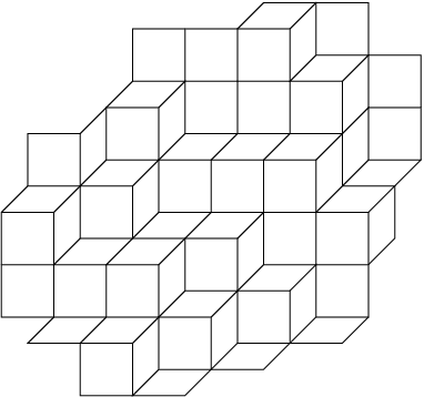
Figure 5: An example of a combinatorial surface Ω𝒟⊂ℤ3\Omega_{\mathscr{D}}\subset\mathds{Z}^{3}.

Any rhombic embedding of a connected b-quad-graph 𝒟{\mathscr{D}} can be seen as a sort of projection of a certain two-dimensional subcomplex (combinatorial surface) Ω𝒟\Omega_{\mathscr{D}} of the multi-dimensional lattice ℤd\mathds{Z}^{d} (or of a multi-dimensional lattice ℒ\cal L which is isomorphic to ℤd\mathds{Z}^{d}). An illustrating example is given in Figure 5.

The combinatorial surface Ω𝒟\Omega_{\mathscr{D}} in ℤd\mathds{Z}^{d} can be constructed in the following way. Denote the set of the different edge directions of 𝒟\mathscr{D} by 𝒜={±a1,…,±ad}⊂𝕊1{\cal A}=\{\pm a_{1},\dots,\pm a_{d}\}\subset\mathds{S}^{1}. We suppose that d>1d>1 and that any two non-opposite elements of 𝒜{\cal A} are linearly independent over ℝ\mathds{R}. Let 𝐞1,…,𝐞d{\mathbf{e}}_{1},\dots,{\mathbf{e}}_{d} denote the standard orthonormal basis of ℝd\mathds{R}^{d}. Fix a white vertex x0∈V⁡(𝒟)x_{0}\in V({\mathscr{D}}) and the origin of ℝd\mathds{R}^{d}. Add the edges of {±𝐞1,…,±𝐞d}\{\pm{\mathbf{e}}_{1},\dots,\pm{\mathbf{e}}_{d}\} at the origin which correspond to the edges of {±a1,…,±ad}\{\pm a_{1},\dots,\pm a_{d}\} incident to x0x_{0} in 𝒟\mathscr{D}, together with their endpoints. Successively continue the construction at the new endpoints. Also, add two-dimensional facets (faces) of ℤd\mathds{Z}^{d} corresponding to faces of 𝒟\mathscr{D}, spanned by incident edges.

A combinatorial surface Ω𝒟\Omega_{\mathscr{D}} in ℤd\mathds{Z}^{d} corresponding to a quasicrystallic rhombic embedding can be characterized using the following monotonicity property, see [BMS05, Section 6] for a proof.

Lemma 4.1 (Monotonicity criterium).

Any two points of Ω𝒟\Omega_{\mathscr{D}} can be connected by a path in Ω𝒟\Omega_{\mathscr{D}} with all directed edges lying in one dd-dimensional octant, that is all directed edges of this path are elements of one of the 2d2^{d} subsets of {±𝐞1,…,±𝐞d}\{\pm{\mathbf{e}}_{1},\dots,\pm{\mathbf{e}}_{d}\} containing dd linearly independent vectors.

An important class of examples of rhombic embeddings of b-quadgraphs can be constructed using ideas of the grid projection method for quasiperiodic tilings of the plane; see for example [DK85, GR86, Sen95].

Example 4.2 (Quasicrystallic rhombic embedding obtained from a plane).

Let EE be a two-dimensional plane in ℝd\mathds{R}^{d} and t∈Et\in E. Let 𝐞1,…,𝐞d{\mathbf{e}}_{1},\dots,{\mathbf{e}}_{d} be the standard orthonormal basis of ℝd\mathds{R}^{d}. We assume that EE does not contain any of the segments sj={𝐭+λ​𝐞j:λ∈[0,1]}s_{j}=\{{\mathbf{t}}+\lambda{\mathbf{e}}_{j}:\lambda\in[0,1]\} for j=1,…,dj=1,\dots,d. Then we can choose positive numbers c1,…,cdc_{1},\dots,c_{d} such that the orthogonal projections PE​(cj​𝐞j)P_{E}(c_{j}{\mathbf{e}}_{j}) have length 1. (If EE contains two different segments sj1s_{j_{1}} and sj2s_{j_{2}}, the following construction only leads to the standard square grid pattern ℤ2\mathds{Z}^{2}. If EE contains exactly one such segment sjs_{j}, then the construction may be adapted for the remaining dimensions excluding 𝐞j{\mathbf{e}}_{j}.) We further assume that the orthogonal projections onto EE of the two-dimensional facets Ej1,j2={λ1𝐞j1+λ2𝐞j2:λ1,λ2∈[0,1]}E_{j_{1},j_{2}}=\{\lambda_{1}{\mathbf{e}}_{j_{1}}+\lambda_{2}{\mathbf{e}}_{j_{2}}:\lambda_{1},\lambda_{2}\in[0,1]\} for 1≤j1<j2≤d1\leq j_{1}<j_{2}\leq d are non-degenerate parallelograms.

Consider around each vertex 𝐩{\mathbf{p}} of the lattice ℒ=c1​ℤ×⋯×cd​ℤ{\cal L}=c_{1}\mathds{Z}\times\dots\times c_{d}\mathds{Z} the hypercuboid V=[−c1/2,c1/2]×⋯×[−cd/2,cd/2]V=[-c_{1}/2,c_{1}/2]\times\dots\times[-c_{d}/2,c_{d}/2], that is the Voronoi cell 𝐩+V{\mathbf{p}}+V. These translations of VV cover ℝd\mathds{R}^{d}. We build an infinite monotone two-dimensional surface Ωℒ​(E)\Omega^{\cal L}(E) in ℒ{\cal L} by the following construction. The basic idea is illustrated in Figure 6 (left).

If EE intersects the interior of the Voronoi cell of a lattice point (i.e. (𝐩+V)∘∩E≠∅({\mathbf{p}}+V)^{\circ}\cap E\not=\emptyset for 𝐩∈ℒ{\mathbf{p}}\in{\cal L}), then this point belongs to Ωℒ​(E)\Omega^{\cal L}(E). Undirected edges correspond to intersections of EE with the interior of a (d−1)(d-1)-dimensional facet bounding two Voronoi cells. Thus we get a connected graph in ℒ{\cal L}. An intersection of EE with the interior of a translated (d−2)(d-2)-dimensional facet of VV corresponds to a rectangular two-dimensional face of the lattice. By construction, the orthogonal projection of this graph onto EE results in a planar connected graph whose faces are all of even degree (== number of incident edges or of incident vertices). A face of degree bigger than 4 corresponds to an intersection of EE with the translation of a (d−k)(d-k)-dimensional facet of VV for some k≥3k\geq 3. Consider the vertices and edges of such a face and the corresponding points and edges in the lattice ℒ{\cal L}. These points lie on a combinatorial kk-dimensional hypercuboid contained in ℒ{\cal L}. By construction, it is easy to see that there are two points of the kk-dimensional hypercuboid which are each incident to kk of the given vertices. We choose a point with least distance from EE and add it to the surface. Adding edges to neighboring vertices splits the face of degree 2​k2k into kk faces of degree 4. Thus we obtain an infinite monotone two-dimensional combinatorial surface Ωℒ​(E)\Omega^{\cal L}(E) which projects to an infinite rhombic embedding covering the whole plane EE.

E ⁢ Ω L ( E )
(a) Straight line EE.
E △ ⁢ Ω L ( E △ )
(b) Modified line E△E_{\triangle} with a “hat”.
Figure 6: Example for the usage of the grid-projection method in ℤ2\mathds{Z}^{2}. The Voronoi cells which contain Ωℒ\Omega^{\cal L} are marked in red.
Example 4.3 (Modification of the construction in Example 4.2).

The method used in the preceding example can be modified to result in similar but different rhombic embeddings. The basic idea is illustrated in Figure 6 (right).

Let EE be a two-dimensional plane in ℝd\mathds{R}^{d} satisfying the same assumptions as in Example 4.2. Let 𝐍≠0{\mathbf{N}}\not=0 be a vector orthogonal to EE. Let △\triangle be an equilateral triangle in EE with vertices 𝐭1,𝐭2,𝐭3{\mathbf{t}}_{1},{\mathbf{t}}_{2},{\mathbf{t}}_{3} and let 𝐬\mathbf{s} be the intersection point of the bisecting lines of the angles. Consider the two-dimensional facets of the three-dimensional tetrahedron T⁡(△,𝐍)T(\triangle,{\mathbf{N}}) spanned by the four vertices 𝐭1,𝐭2,𝐭3,𝐬+𝐍{\mathbf{t}}_{1},{\mathbf{t}}_{2},{\mathbf{t}}_{3},{\mathbf{s}}+{\mathbf{N}}. Exactly one of these facets is completely contained in EE (this is the triangle △\triangle). We remove the triangle from EE and add instead the remaining facets of T⁡(△,𝐍)T(\triangle,{\mathbf{N}}). Let E△E_{\triangle} be the resulting two-dimensional surface. Note that E△E_{\triangle} is orientable like EE. Define γ∈(0,π/2)\gamma\in(0,\pi/2) by γ=arctan⁡(2​3​‖𝐍‖/‖𝐭1−𝐭2‖)\gamma=\arctan(2\sqrt{3}\|{\mathbf{N}}\|/\|{\mathbf{t}}_{1}-{\mathbf{t}}_{2}\|), where ∥⋅∥\|\cdot\| denotes the Euclidean norm of vectors in ℝd\mathds{R}^{d}. γ\gamma is the acute angle between EE and the two-dimensional facets of T⁡(△,𝐍)T(\triangle,{\mathbf{N}}) not contained in EE.

If γ\gamma is small enough, then our assumptions imply that we can apply the same construction algorithm to E△E_{\triangle} as for the plane EE in the previous example and obtain a monotone surface Ωℒ​(E△)\Omega^{\cal L}(E_{\triangle}). The orthogonal projection of Ωℒ​(E△)\Omega^{\cal L}(E_{\triangle}) onto EE is a rhombic embedding which coincides with the rhombic embedding from Ωℒ​(E)\Omega^{\cal L}(E) except for a finite part.

The quasicrystallic rhombic embedding of Example 4.3 may also obtained using the following general concept of local changes of rhombic embeddings.

Definition 4.4.

Let 𝒟{\mathscr{D}} be a rhombic embedding of a finite simply connected b-quad-graph with corresponding combinatorial surface Ω𝒟\Omega_{\mathscr{D}} in ℤd\mathds{Z}^{d}.

Refer to caption
Figure 7: A flip of a three-dimensional cube. The dashed edges and their incident faces are not part of the surface in ℤd\mathds{Z}^{d}.

Let 𝐳^∈Vi​n​t​(Ω𝒟)\hat{\mathbf{z}}\in V_{int}(\Omega_{\mathscr{D}}) be an interior vertex with exactly three incident two-dimensional facets of Ω𝒟\Omega_{\mathscr{D}}. Consider the three-dimensional cube with these boundary facets. Replace the three given facets with the three other two-dimensional facets of this cube. This procedure is called a flip; see Figure 7 for an illustration.

A vertex 𝐳∈ℤd{\mathbf{z}}\in\mathds{Z}^{d} can be reached with flips from Ω𝒟\Omega_{\mathscr{D}} if 𝐳{\mathbf{z}} is contained in a combinatorial surface obtained from Ω𝒟\Omega_{\mathscr{D}} by a suitable sequence of flips. The set of all vertices which can be reached with flips (including V⁡(Ω𝒟)V(\Omega_{\mathscr{D}})) will be denoted by ℱ⁡(Ω𝒟){\cal F}(\Omega_{\mathscr{D}}).

For further use we enlarge the set ℱ⁡(Ω𝒟){\cal F}(\Omega_{\mathscr{D}}) of vertices which can be reached by flips from Ω𝒟\Omega_{\mathscr{D}} in the following way. For a set of vertices W⊂V⁡(ℤd)W\subset V(\mathds{Z}^{d}) denote by W[1]W^{[1]} the set WW together with all vertices incident to a two-dimensional facet of ℤd\mathds{Z}^{d} where three of its four vertices belong to WW. Define W[k+1]=(W[k])[1]W^{[k+1]}=(W^{[k]})^{[1]} inductively for all k∈ℕk\in\mathds{N}. In particular, we denote for some arbitrary, but fixed κ∈ℕ\kappa\in\mathds{N}

ℱκ​(Ω𝒟)=(ℱ⁡(Ω𝒟))[κ].{\cal F}_{\kappa}(\Omega_{\mathscr{D}})=({\cal F}(\Omega_{\mathscr{D}}))^{[\kappa]}.

4.2 Quasicrystallic circle patterns and integrability

Let 𝒟\mathscr{D} be a quasicrystallic rhombic embedding of a b-quad-graph. The combinatorial surface Ω𝒟\Omega_{\mathscr{D}} in ℤd\mathds{Z}^{d} is important by its connection with integrability. See also [BS08] for a more detailed presentation and a deepened study of integrability and consistency.

In particular, a function defined on the vertices of Ω𝒟\Omega_{\mathscr{D}} which satisfies some 3D-consistent equation on all faces of Ω𝒟\Omega_{\mathscr{D}} can uniquely be extended to the brick

Π(Ω𝒟):={𝐧=(n1,…,nd)∈ℤd:ak(Ω𝒟)≤nk≤bk(Ω𝒟),k=1,…,d},\Pi(\Omega_{\mathscr{D}}):=\{{\mathbf{n}}=(n_{1},\dots,n_{d})\in\mathds{Z}^{d}:a_{k}(\Omega_{\mathscr{D}})\leq n_{k}\leq b_{k}(\Omega_{\mathscr{D}}),\ k=1,\dots,d\},

where ak​(Ω𝒟)=min𝐧∈V⁡(Ω𝒟)⁡nka_{k}(\Omega_{\mathscr{D}})=\min_{{\mathbf{n}}\in V(\Omega_{\mathscr{D}})}n_{k} and bk​(Ω𝒟)=max𝐧∈V⁡(Ω𝒟)⁡nkb_{k}(\Omega_{\mathscr{D}})=\max_{{\mathbf{n}}\in V(\Omega_{\mathscr{D}})}n_{k}. Note that Π⁡(Ω𝒟)\Pi(\Omega_{\mathscr{D}}) is the hull of Ω𝒟\Omega_{\mathscr{D}}. A proof may be found in [BMS05, Section 6]. This extension of a function using a 3D-consistent equation will now be applied for the comparison function ww defined in (14) of two circle patterns. In particular, we take for 𝒞1{\mathscr{C}}_{1} the isoradial circle pattern which corresponds to the quasicrystallic rhombic embedding 𝒟\mathscr{D}. Given another circle pattern 𝒞2{\mathscr{C}}_{2} for 𝒟\mathscr{D} with the same intersection angles, let ww be the comparison function for 𝒞2{\mathscr{C}}_{2}. Note that the Hirota Equation (15) is 3D-consistent; see Sections 10 and 11 of [BMS05] for more details. Thus ww considered as a function on V⁡(Ω𝒟)V(\Omega_{\mathscr{D}}) can uniquely be extended to the brick Π⁡(Ω𝒟)\Pi(\Omega_{\mathscr{D}}) such that equation (15) holds on all two-dimensional facets. Additionally, ww and its extension are real valued on white points Vw​(Ω𝒟)V_{w}(\Omega_{\mathscr{D}}) and has value in 𝕊1\mathds{S}^{1} for black points Vb​(Ω𝒟)V_{b}(\Omega_{\mathscr{D}}). This can easily be deduced from the Hirota Equation (15).

The extension of ww can be used to define a radius function for any rhombic embedding with the same boundary faces as 𝒟\mathscr{D}.

Lemma 4.5.

Let 𝒟{\mathscr{D}} and 𝒟′{\mathscr{D}}^{\prime} be two simply connected finite rhombic embeddings of b-quad-graphs with the same edge directions. Assume that 𝒟{\mathscr{D}} and 𝒟′{\mathscr{D}}^{\prime} agree on all boundary faces. Let 𝒞{\mathscr{C}} be an (embedded) planar circle pattern for 𝒟{\mathscr{D}} and the labelling given by the rhombic embedding. Then there is an (embedded) planar circle pattern 𝒞′{\mathscr{C}}^{\prime} for 𝒟′{\mathscr{D}}^{\prime} which agrees with 𝒞{\mathscr{C}} for all boundary circles.

Proof.

Consider the monotone combinatorial surfaces Ω𝒟\Omega_{\mathscr{D}} and Ω𝒟′\Omega_{\mathscr{D}}^{\prime}. Without loss of generality, we can assume that Ω𝒟\Omega_{\mathscr{D}} and Ω𝒟′\Omega_{\mathscr{D}}^{\prime} have the same boundary faces in ℤd\mathds{Z}^{d}. Thus they both define the same brick Π⁡(Ω𝒟)=Π⁡(Ω𝒟′)=:Π\Pi(\Omega_{\mathscr{D}})=\Pi(\Omega_{\mathscr{D}}^{\prime})=:\Pi. Given the circle pattern 𝒞{\mathscr{C}}, define the function ww on V⁡(Ω𝒟)V(\Omega_{\mathscr{D}}) by (14). Extend ww to the brick Π\Pi such that condition (15) holds for all two-dimensional facets. Consider ww on Ω𝒟′\Omega_{\mathscr{D}}^{\prime} and build the corresponding pattern 𝒞′{\mathscr{C}}^{\prime}, such that the points on the boundary agree with those of the given circle pattern 𝒞{\mathscr{C}}. Equation (15) guarantees that all rhombi of Ω𝒟′\Omega_{\mathscr{D}}^{\prime} are mapped to closed kites. Due to the combinatorics, the chain of kites is closed around each vertex. Since the boundary kites of 𝒞′{\mathscr{C}}^{\prime} are given by 𝒞{\mathscr{C}} which is an immersed circle pattern, at every interior white point the angles of the kites sum up to 2​π2\pi. Thus 𝒞′{\mathscr{C}}^{\prime} is an immersed circle pattern.

Furthermore, 𝒞′{\mathscr{C}}^{\prime} is embedded if 𝒞{\mathscr{C}} is, because 𝒞′{\mathscr{C}}^{\prime} is an immersed circle pattern and 𝒞′{\mathscr{C}}^{\prime} and 𝒞{\mathscr{C}} agree for all boundary kites. ∎

5 C∞C^{\infty}-convergence for quasicrystallic circle patterns

In order to improve the order of convergence in Theorem 3.1 we study partial derivatives of the extended radius function using the integrability of the Hirota equation (15) and a Regularity Lemma 5.6.

The following constants are useful to estimate the possible orders of partial derivatives for a function defined on ℱκ​(Ω𝒟){\cal F}_{\kappa}(\Omega_{\mathscr{D}}). Note that ℱκ​(Ω𝒟)⊂Π⁡(Ω𝒟){\cal F}_{\kappa}(\Omega_{\mathscr{D}})\subset\Pi(\Omega_{\mathscr{D}}).

Definition 5.1.

Let 𝒟{\mathscr{D}} be a rhombic embedding of a finite simply connected b-quad-graph with corresponding combinatorial surface Ω𝒟\Omega_{\mathscr{D}} in ℤd\mathds{Z}^{d}. Let J⊂{1,…,d}J\subset\{1,\dots,d\} contain at least two different indices.

For B≥0B\geq 0 define a combinatorial ball of radius BB about 𝐳∈V⁡(ℤd){\mathbf{z}}\in V(\mathds{Z}^{d}) using the directions {𝐞j:j∈J}\{\mathbf{e}_{j}:j\in J\} by

UJ​(𝐳,B)={ζ=𝐳+∑j∈Jnj​𝐞j:∑j∈J|nj|≤B}.U_{J}({\mathbf{z}},B)=\{{\mathbf{\zeta}}={\mathbf{z}}+\sum_{j\in J}n_{j}\mathbf{e}_{j}:\sum_{j\in J}|n_{j}|\leq B\}. (38)

The radius of the largest ball about 𝐳{\mathbf{z}} using these directions which is contained in ℱκ​(Ω𝒟){\cal F}_{\kappa}(\Omega_{\mathscr{D}}) is denoted by BJ​(𝐳,ℱκ​(Ω𝒟))=max⁡{B∈ℕ:UJ​(𝐳,B)⊂ℱκ​(Ω𝒟)}B_{J}({\mathbf{z}},{\cal F}_{\kappa}(\Omega_{\mathscr{D}}))=\max\{B\in\mathds{N}:U_{J}({\mathbf{z}},B)\subset{\cal F}_{\kappa}(\Omega_{\mathscr{D}})\}.

Denote by d⁡(𝐳^,∂Ω𝒟)d(\hat{\mathbf{z}},\partial\Omega_{\mathscr{D}}) the combinatorial distance of 𝐳^∈V⁡(Ω𝒟)\hat{\mathbf{z}}\in V(\Omega_{\mathscr{D}}) to the boundary ∂Ω𝒟\partial\Omega_{\mathscr{D}}, that is the smallest integer KK such that there is a connected path with KK edges contained in Ω𝒟\Omega_{\mathscr{D}} from 𝐳^\hat{\mathbf{z}} to a boundary vertex of ∂Ω𝒟\partial\Omega_{\mathscr{D}}. For further use, we define the constant

CJ​(ℱκ​(Ω𝒟))=min⁡{BJ​(𝐳^,ℱκ​(Ω𝒟))+1d⁡(𝐳^,∂Ω𝒟):𝐳^∈Vi​n​t​(Ω𝒟)}>0.C_{J}({\cal F}_{\kappa}(\Omega_{\mathscr{D}}))=\min\left\{\frac{B_{J}(\hat{\mathbf{z}},{\cal F}_{\kappa}(\Omega_{\mathscr{D}}))+1}{d(\hat{\mathbf{z}},\partial\Omega_{\mathscr{D}})}:\hat{\mathbf{z}}\in V_{int}(\Omega_{\mathscr{D}})\right\}>0. (39)

Note as an immediate consequence that for all 𝐳^∈Vi​n​t​(Ω𝒟)\hat{\mathbf{z}}\in V_{int}(\Omega_{\mathscr{D}})

UJ​(𝐳^,⌈CJ​(ℱκ​(Ω𝒟))​d​(𝐳^,∂Ω𝒟)−1⌉)⊂ℱκ​(Ω𝒟),U_{J}(\hat{\mathbf{z}},\lceil C_{J}({\cal F}_{\kappa}(\Omega_{\mathscr{D}}))d(\hat{\mathbf{z}},\partial\Omega_{\mathscr{D}})-1\rceil)\subset{\cal F}_{\kappa}(\Omega_{\mathscr{D}}),

where ⌈s⌉\lceil s\rceil denotes the smallest integer bigger than s∈ℝs\in\mathds{R}.

The following theorem is an improved version of Theorem 3.1 for a specified class of quasicrystallic circle patterns.

Theorem 5.2.

Under the assumptions of Theorem 3.1 and with the same notation, let d∈ℕd\in\mathds{N} with d≥2d\geq 2 be a constant and assume further that 𝒟n{\mathscr{D}}_{n} is a quasicrystallic rhombic embedding in DD with edge lengths εn\varepsilon_{n} and dimension dn≤dd_{n}\leq d. The directions of the edges are elements of the set {±a1(n),…,±adn(n)}⊂𝕊1\{\pm a_{1}^{(n)},\dots,\pm a_{d_{n}}^{(n)}\}\subset\mathds{S}^{1} such that any two of the vectors of {a1(n),…,adn(n)}\{a_{1}^{(n)},\dots,a_{d_{n}}^{(n)}\} are linearly independent. The possible angles are uniformly bounded, that is for all n∈ℕn\in\mathds{N} the scalar product is strictly bounded away from 11,

|⟨ai(n),aj(n)⟩|≤cos⁡(π/2+C)<1,|\langle a_{i}^{(n)},a_{j}^{(n)}\rangle|\leq\cos(\pi/2+C)<1, (40)

for all 1≤i<j≤dn1\leq i<j\leq d_{n} and some constant 0<C<π/20<C<\pi/2. Consequently, the intersection angles αn\alpha_{n} are uniformly bounded in the sense that for all n∈ℕn\in\mathds{N} and all faces f∈F⁡(𝒟n)f\in F({\mathscr{D}}_{n}) there holds

|αn​(f)−π/2|≤C.|\alpha_{n}(f)-\pi/2|\leq C. (41)

Let κ∈ℕ\kappa\in\mathds{N}, let J0⊂{1,…,d}J_{0}\subset\{1,\dots,d\} contain at least two indices, and let B,CJ0>0B,C_{J_{0}}>0 be real constants. Suppose that J0⊂{1,…,dn}J_{0}\subset\{1,\dots,d_{n}\} for all n∈ℕn\in\mathds{N} and

CJ0​(ℱκ​(Ω𝒟n))≥CJ0>0.C_{J_{0}}({\cal F}_{\kappa}(\Omega_{{\mathscr{D}}_{n}}))\geq C_{J_{0}}>0.

Then we have with the same definitions of rnr_{n}, ϕn\phi_{n}, qnq_{n}, and pnp_{n} as in Theorem 3.1 that qn→g′q_{n}\to g^{\prime} and gn→gg_{n}\to g in C∞​(D)C^{\infty}(D) as n→∞n\to\infty, that is discrete partial derivatives of all orders of qnq_{n} and gng_{n} converge uniformly on compact subsets to their smooth counterparts.

Simple examples of sequences of quasicrystallic circle patterns for this theorem are subgraphs of the suitably scaled infinite regular square grid or hexagonal circle patterns or subgraphs of suitably scaled infinite rhombic embeddings constructed in Examples 4.2 and 4.3 (see Figure 2). Simply connected parts of these rhombic embeddings which are large enough satisfy the conditions CJ​(ℱκ​(Ω𝒟n))≥C0>0C_{J}({\cal F}_{\kappa}(\Omega_{{\mathscr{D}}_{n}}))\geq C_{0}>0 for all subsets J⊂{1,…,d}J\subset\{1,\dots,d\}, where the constant C0C_{0} only depends on the construction parameters. This is a consequence of the simple combinatorics or of the modified construction in Example 4.3.

Remark 5.3.

Similarly as for Theorem 3.1, the proof of Theorem 5.2 shows that we have in fact a priori bounds in O⁡(εn)O(\varepsilon_{n}) on compact subset of DD for the difference of directional derivatives of log⁡g′\log g^{\prime} (and thus of g′g^{\prime} and gg) and corresponding discrete partial derivatives of log⁡rnεn+i⁡(φn−ϕn)\log\frac{r_{n}}{\varepsilon_{n}}+i(\varphi_{n}-\phi_{n}) (and thus qnq_{n} and gng_{n} respectively). The constant in the estimation depends on the order of the partial derivatives and on the compact subset.

Furthermore, for the ’very regular’ case considered in Remark 3.4 the a priori bounds on the above partial derivatives have order O⁡(εn2)O(\varepsilon_{n}^{2}) on compact subset of DD due to the improved estimation (29).

Remark 5.4.

There is an analogous version of Theorem 5.2 of C∞C^{\infty}-convergence for quasicrystallic circle patterns with Neumann boundary conditions.

For the proof of Theorem 5.2, we first define the comparison function wnw_{n} for the circle pattern 𝒞n{\mathscr{C}}_{n} according to (14) and extend it to ℱκ​(Ω𝒟n){\cal F}_{\kappa}(\Omega_{{\mathscr{D}}_{n}}). This extension is again denoted by wnw_{n}. The restriction of wnw_{n} to white vertices is called extended radius function and denoted by rnr_{n} as the original radius function for 𝒞n{\mathscr{C}}_{n}. We also extend |g′||g^{\prime}| to ℱκ​(Ω𝒟n){\cal F}_{\kappa}(\Omega_{{\mathscr{D}}_{n}}) by defining |g′​(𝐳)||g^{\prime}({\mathbf{z}})| to be the value |g′​(z)||g^{\prime}(z)| at the projection zz of 𝐳∈ℤd{\mathbf{z}}\in\mathds{Z}^{d} onto the plane of the rhombic embedding 𝒟n{\mathscr{D}}_{n}. If nn is big enough, which will be assumed in the following, then z∈Dz\in D or z∈W∖Dz\in W\setminus D and the distance of zz to DD is bounded independently of nn.

Denote tn=log⁡(rn/Rn)=log⁡(rn/εn)t_{n}=\log(r_{n}/R_{n})=\log(r_{n}/\varepsilon_{n}) and hn=log⁡|g′|h_{n}=\log|g^{\prime}| as in Section 3. Using the extensions of rnr_{n} and |g′||g^{\prime}|, these functions are defined on all white vertices of ℱκ​(Ω𝒟n){\cal F}_{\kappa}(\Omega_{{\mathscr{D}}_{n}}). Furthermore we have the following extension of Lemma 3.3.

Lemma 5.5.

The estimation

hn​(𝐳)−tn​(𝐳)=𝒪⁡(εn).h_{n}({\mathbf{z}})-t_{n}({\mathbf{z}})={\cal O}(\varepsilon_{n}).

holds for all white vertices 𝐳∈V⁡(ℱκ​(Ω𝒟n)){\mathbf{z}}\in V({\cal F}_{\kappa}(\Omega_{{\mathscr{D}}_{n}})). The constant in the 𝒪{\cal O}-notation may depend on κ\kappa and on the dimension dnd_{n} of 𝒟n{\mathscr{D}}_{n}.

Proof.

Let 𝐳∈V⁡(ℱ⁡(Ω𝒟n)){\mathbf{z}}\in V({\cal F}(\Omega_{{\mathscr{D}}_{n}})) be a white vertex. By definition of ℱ⁡(Ω𝒟n){\cal F}(\Omega_{{\mathscr{D}}_{n}}) there is a combinatorial surface Ω′​(𝐳)\Omega^{\prime}({\mathbf{z}}) containing 𝐳{\mathbf{z}} with the same boundary curve as Ω𝒟n\Omega_{{\mathscr{D}}_{n}}. Lemma 4.5 implies that we can define an embedded circle pattern 𝒞′{\mathscr{C}}^{\prime} using the values of wnw_{n} on Ω𝒟n\Omega_{{\mathscr{D}}_{n}}. Now the claim follows from Lemma 3.3.

For 𝐳∈V⁡(ℱκ​(Ω𝒟n))∖V⁡(ℱ⁡(Ω𝒟n)){\mathbf{z}}\in V({\cal F}_{\kappa}(\Omega_{{\mathscr{D}}_{n}}))\setminus V({\cal F}(\Omega_{{\mathscr{D}}_{n}})) observe that equation (15) may be used to extend the estimation of hn−tnh_{n}-t_{n}. Each steps adds an error of order εn\varepsilon_{n}, therefore the final constant depends on κ\kappa and on dnd_{n}. ∎

Our main aim is to estimate the partial derivatives of the extended radius function in ℤdn\mathds{Z}^{d_{n}}. Such partial derivatives can generally be considered in direction of the vectors 𝐯=±𝐞j1±𝐞j2{\mathbf{v}}=\pm{\mathbf{e}}_{j_{1}}\pm{\mathbf{e}}_{j_{2}} for 0≤j1,j2≤dn0\leq j_{1},j_{2}\leq d_{n} such that 𝐞j1{\mathbf{e}}_{j_{1}} and 𝐞j2{\mathbf{e}}_{j_{2}} are not collinear. Let 𝐯1,…,𝐯2​dn​(dn−1){\mathbf{v}}_{1},\dots,{\mathbf{v}}_{2d_{n}(d_{n}-1)} be an enumeration of these vectors and set 𝐕n={𝐯1,…,𝐯2​dn​(dn−1)}{\mathbf{V}}_{n}=\{{\mathbf{v}}_{1},\dots,{\mathbf{v}}_{2d_{n}(d_{n}-1)}\}. The corresponding enumeration of the directions v=±aj1(n)±aj2(n)v=\pm{a}_{j_{1}}^{(n)}\pm{a}_{j_{2}}^{(n)} in 𝒟n{\mathscr{D}}_{n} for 0≤j1,j2≤d0\leq j_{1},j_{2}\leq d is denoted by v1,…​v2​dn​(dn−1)v_{1},\dots v_{2d_{n}(d_{n}-1)}.

For any function hh on white vertices 𝐳∈ℤd{\mathbf{z}}\in\mathds{Z}^{d} and/or in z∈ℂz\in\mathds{C} define discrete partial derivatives in direction 𝐯i{\mathbf{v}}_{i} or viv_{i} by

∂𝐯ih⁡(𝐳)\displaystyle\partial_{{\mathbf{v}}_{i}}h({\mathbf{z}}) =h⁡(𝐳+𝐯i)−h⁡(𝐳)εn​|vi|and∂vih(z)=h⁡(z+εn​vi)−h⁡(z)εn​|vi|\displaystyle=\frac{h({\mathbf{z}}+{\mathbf{v}}_{i})-h({\mathbf{z}})}{\varepsilon_{n}|v_{i}|}\hskip 20.00003pt\text{and}\hskip 20.00003pt\partial_{{v}_{i}}h({z})=\frac{h({z}+\varepsilon_{n}{v}_{i})-h({z})}{\varepsilon_{n}|v_{i}|}

respectively. Furthermore, we call a direction 𝐯i{\mathbf{v}}_{i} or viv_{i} to be contained in Ω𝒟n\Omega_{{\mathscr{D}}_{n}} or 𝒟n{\mathscr{D}}_{n} at a vertex 𝐳^\hat{\mathbf{z}} or zz respectively if there is a two-dimensional facet of Ω𝒟n\Omega_{{\mathscr{D}}_{n}} incident to 𝐳^\hat{\mathbf{z}} whose diagonal incident to 𝐳^\hat{\mathbf{z}} is parallel to 𝐯i{\mathbf{v}}_{i}, that is {𝐳^+λ​𝐯i:λ∈[0,1]}⊂Ω𝒟n\{\hat{\mathbf{z}}+\lambda{\mathbf{v}}_{i}:\lambda\in[0,1]\}\subset\Omega_{{\mathscr{D}}_{n}}.

Corresponding to these partial derivatives we use a scaled version of the Laplacian in (30). For a function η\eta and an interior vertex zz with incident vertices z1,…,zLz_{1},\dots,z_{L} define the discrete Laplacian by

Δεn​η​(z):=Δ𝐯μ1,…,𝐯μLεn​η​(z):=1εn2​∑j=1L2​fαn​([z,zj])′​(0)​(η⁡(zj)−η⁡(z)).\Delta^{\varepsilon_{n}}\eta(z):=\Delta^{\varepsilon_{n}}_{{\mathbf{v}}_{\mu_{1}},\dots,{\mathbf{v}}_{\mu_{L}}}\eta(z):=\frac{1}{\varepsilon_{n}^{2}}\sum_{j=1}^{L}2f^{\prime}_{\alpha_{n}([z,z_{j}])}(0)(\eta(z_{j})-\eta(z)). (42)

Here vμj=v⁡([z,zj])=(zj−z)/εnv_{\mu_{j}}=v([z,z_{j}])=(z_{j}-z)/\varepsilon_{n} (j=1,…,Lj=1,\dots,L) and the notation Δ𝐯μ1,…,𝐯μLεn\Delta^{\varepsilon_{n}}_{{\mathbf{v}}_{\mu_{1}},\dots,{\mathbf{v}}_{\mu_{L}}} emphasizes the dependence of the Laplacian on the directions v⁡([z,zj])v([z,z_{j}]) of the edges [z,zj]∈E⁡(Gn)[z,z_{j}]\in E(G_{n}).

Let z0∈Vi​n​t​(Gn)z_{0}\in V_{int}(G_{n}) be an interior vertex and let 𝐯μ1,…,𝐯μL∈𝐕n{\mathbf{v}}_{\mu_{1}},\dots,{\mathbf{v}}_{\mu_{L}}\in{\mathbf{V}}_{n} be the directions which correspond to the directions of the edges of GnG_{n} incident to z0z_{0}. Let 𝐳1∈ℱκ​(Ω𝒟n){\mathbf{z}}_{1}\in{\cal F}_{\kappa}(\Omega_{{\mathscr{D}}_{n}}) be a vertex such that 𝐳1+𝐯μi∈ℱκ​(Ω𝒟n){\mathbf{z}}_{1}+{\mathbf{v}}_{\mu_{i}}\in{\cal F}_{\kappa}(\Omega_{{\mathscr{D}}_{n}}) for all i=1,…,Li=1,\dots,L. Our next aim is to study Δ𝐯μ1,…,𝐯μLεn​tn​(𝐳1)\Delta^{\varepsilon_{n}}_{{\mathbf{v}}_{\mu_{1}},\dots,{\mathbf{v}}_{\mu_{L}}}t_{n}({\mathbf{z}}_{1}). For this purpose we assume that we have translated to 𝐳1{\mathbf{z}}_{1} the facets of Ω𝒟n\Omega_{{\mathscr{D}}_{n}} incident to 𝐳0{\mathbf{z}}_{0}, that is we consider the (very small) monotone surface consisting of the two-dimensional facets incident to 𝐳1{\mathbf{z}}_{1} which contain a diagonal {𝐳1+λ​𝐯μi:λ∈[0,1]}\{{\mathbf{z}}_{1}+\lambda{\mathbf{v}}_{\mu_{i}}:\lambda\in[0,1]\} for i=1,…,Li=1,\dots,L. Using the extension of the comparison function wnw_{n}, the closed chain of these two-dimensional facets incident to 𝐳1{\mathbf{z}}_{1} is mapped to a closed chain of kites. Thus we have

∑l=1L2​fαμl​(tn​(𝐳1+𝐯μl)−tn​(𝐳1))∈2​π​ℕ,\sum_{l=1}^{L}2f_{\alpha_{\mu_{l}}}(t_{n}({\mathbf{z}}_{1}+{\mathbf{v}}_{\mu_{l}})-t_{n}({\mathbf{z}}_{1}))\in 2\pi\mathds{N},

where αμl\alpha_{\mu_{l}} denotes the labelling of the two-dimensional facet containing 𝐳1{\mathbf{z}}_{1} and 𝐳1+𝐯μl{\mathbf{z}}_{1}+{\mathbf{v}}_{\mu_{l}}. By assumption ∑l=1L2​fαμl​(0)=2​π\sum_{l=1}^{L}2f_{\alpha_{\mu_{l}}}(0)=2\pi and we know that tn​(𝐳1+𝐯μl)−tn​(𝐳1)=𝒪⁡(εn)t_{n}({\mathbf{z}}_{1}+{\mathbf{v}}_{\mu_{l}})-t_{n}({\mathbf{z}}_{1})={\cal O}(\varepsilon_{n}) by Lemma 5.5. Since the intersection angles and thus the maximum number of neighbors are uniformly bounded, we deduce that

(∑l=1L2​fαμl​(tn​(𝐳1+𝐯μl)−tn​(𝐳1)))−2​π=0\Biggl(\sum_{l=1}^{L}2f_{\alpha_{\mu_{l}}}(t_{n}({\mathbf{z}}_{1}+{\mathbf{v}}_{\mu_{l}})-t_{n}({\mathbf{z}}_{1}))\Biggr)-2\pi=0

if εn\varepsilon_{n} is small enough. Using a Taylor expansion about 00, we obtain

Δ𝐯μ1,…,𝐯μLεn​tn​(𝐳1)\displaystyle\Delta^{\varepsilon_{n}}_{{\mathbf{v}}_{\mu_{1}},\dots,{\mathbf{v}}_{\mu_{L}}}t_{n}({\mathbf{z}}_{1}) =2εn2(−∑l=1L∑m=3∞fαμl(m)​(0)m!(tn(𝐳1+𝐯μl)−tn(z))m)\displaystyle=\frac{2}{\varepsilon_{n}^{2}}\left(-\sum_{l=1}^{L}\sum_{m=3}^{\infty}\frac{f^{(m)}_{\alpha_{\mu_{l}}}(0)}{m!}(t_{n}({\mathbf{z}}_{1}+{\mathbf{v}}_{\mu_{l}})-t_{n}(z))^{m}\right)
=εn(−2∑l=1L∑m=3∞fαμl(m)​(0)m!|vμl|m(∂𝐯μltn(𝐳1))mεnm−3)\displaystyle=\varepsilon_{n}\left(-2\sum_{l=1}^{L}\sum_{m=3}^{\infty}\frac{f^{(m)}_{\alpha_{\mu_{l}}}(0)}{m!}|v_{\mu_{l}}|^{m}(\partial_{{\mathbf{v}}_{\mu_{l}}}t_{n}({\mathbf{z}}_{1}))^{m}\varepsilon_{n}^{m-3}\right)
=:εn​F𝐯μ1,…,𝐯μL​(εn,∂𝐯μ1tn,…,∂𝐯μLtn,𝐳1),\displaystyle=:\varepsilon_{n}F_{{\mathbf{v}}_{\mu_{1}},\dots,{\mathbf{v}}_{\mu_{L}}}(\varepsilon_{n},\partial_{{\mathbf{v}}_{\mu_{1}}}t_{n},\dots,\partial_{{\mathbf{v}}_{\mu_{L}}}t_{n};{\mathbf{z}}_{1}), (43)

Note that F𝐯μ1,…,𝐯μLF_{{\mathbf{v}}_{\mu_{1}},\dots,{\mathbf{v}}_{\mu_{L}}} is a C∞C^{\infty}-function in the variables εn,∂𝐯μ1tn,…,∂𝐯μLtn\varepsilon_{n},\partial_{{\mathbf{v}}_{\mu_{1}}}t_{n},\dots,\partial_{{\mathbf{v}}_{\mu_{L}}}t_{n}. This fact will be important for the proof of Lemma 5.7 below.

For further use we introduce the following notation. Let KK be a compact subset of DD and let M>0M>0. Denote by Ω𝒟nK,M\Omega_{{\mathscr{D}}_{n}}^{K,M} the part of Ω𝒟n\Omega_{{\mathscr{D}}_{n}} with vertices of combinatorial distance bigger than MM to the boundary and whose corresponding vertices z∈V⁡(𝒟n)z\in V({\mathscr{D}}_{n}) lie in KK. Let J⊂{1,…,d}J\subset\{1,\dots,d\} contain at least two different indices. In order to consider partial derivatives within KK in the directions ±𝐞j1±𝐞j2\pm{\mathbf{e}}_{j_{1}}\pm{\mathbf{e}}_{j_{2}}, where j1,j2∈Jj_{1},j_{2}\in J and j1≠j2j_{1}\not=j_{2}, we attach a ball UJ​(𝐳^,M)U_{J}(\hat{\mathbf{z}},M) at each of these points:

UJ​(K,M,Ω𝒟n)=⋃𝐳^∈V⁡(Ω𝒟nK,M)UJ​(𝐳^,M).U_{J}(K,M,\Omega_{{\mathscr{D}}_{n}})=\bigcup_{\hat{\mathbf{z}}\in V(\Omega_{{\mathscr{D}}_{n}}^{K,M})}U_{J}(\hat{\mathbf{z}},M). (44)

Note that if M≤BJ​(𝐳^)M\leq B_{J}(\hat{\mathbf{z}}), for example if M≤CJ​(ℱκ​(Ω𝒟n))​d​(𝐳^,∂Ω𝒟n)−1M\leq C_{J}({\cal F}_{\kappa}(\Omega_{{\mathscr{D}}_{n}}))d(\hat{\mathbf{z}},\partial\Omega_{{\mathscr{D}}_{n}})-1 for all 𝐳^∈V⁡(Ω𝒟nK,M)\hat{\mathbf{z}}\in V(\Omega_{{\mathscr{D}}_{n}}^{K,M}), then UJ​(K,M,Ω𝒟n)⊂ℱκ​(Ω𝒟n)U_{J}(K,M,\Omega_{{\mathscr{D}}_{n}})\subset{\cal F}_{\kappa}(\Omega_{{\mathscr{D}}_{n}}).

Furthermore we define K+d0K+d_{0} to be the compact d0d_{0}-neighborhood of the compact set K⊂ℂK\subset\mathds{C}, that is

K+d0={z∈ℂ:𝕖⁡(K,z)≤d0},K+d_{0}=\{z\in\mathds{C}:\mathbb{e}(K,z)\leq d_{0}\},

where 𝕖\mathbb{e} denotes the Euclidean distance between a point and a compact set or between two compact subsets of ℂ\mathds{C}.

The following lemma is important for our argumentation, as it gives an estimation of a partial derivative using estimations of the function and its Laplacian.

Lemma 5.6 (Regularity Lemma).

Let 𝒟{\mathscr{D}} be a quasicrystallic rhombic embedding with associated graph GG and labelling α\alpha. Let W⊂V⁡(G)W\subset V(G) and let u:W→ℝu:W\to\mathds{R} be any function. Let M⁡(u)=maxv∈Wi​n​t⁡|Δ​u​(v)/(4​F∗​(v))|M(u)=\max_{v\in W_{int}}|\Delta u(v)/(4F^{*}(v))|, where

F∗​(v)=14​∑[z,v]∈E⁡(G)c⁡([z,v])​|z−v|2=12​∑[z,v]∈E⁡(G)sin⁡α⁡([z,v])F^{*}(v)=\frac{1}{4}\sum_{[z,v]\in E(G)}c([z,v])|z-v|^{2}=\frac{1}{2}\sum_{[z,v]\in E(G)}\sin\alpha([z,v])

is the area of the face of the dual graph G∗G^{*} corresponding to the vertex v∈Vi​n​t​(G)v\in V_{int}(G). There are constants C5,C6>0C_{5},C_{6}>0, independent of WW and uu, such that

|u⁡(x0)−u⁡(x1)|​ρ≤C5​‖u‖W+ρ2​C6​M​(u)|u(x_{0})-u(x_{1})|\rho\leq C_{5}\|u\|_{W}+\rho^{2}C_{6}M(u) (45)

for all vertices x1∈Wx_{1}\in W incident to x0x_{0}, where ρ\rho is the Euclidean distance of x0x_{0} to the boundary W∂W_{\partial}.

A proof is given in the appendix, see Lemma A.8. As a direct application we get

Lemma 5.7.

Let K⊂DK\subset D be a compact set, n0∈ℕn_{0}\in\mathds{N} and 0<d0<𝕖⁡(K,∂𝒟n)0<d_{0}<\mathbb{e}(K,\partial{\mathscr{D}}_{n}) for all n≥n0n\geq n_{0}.

Let k∈ℕ0k\in\mathds{N}_{0} and let 𝐯i1,…,𝐯ik∈⋂n≥n0𝐕n{\mathbf{v}}_{i_{1}},\dots,{\mathbf{v}}_{i_{k}}\in\bigcap_{n\geq n_{0}}{\mathbf{V}}_{n} be kk not necessarily different directions. Let J⊂{1,…,d}J\subset\{1,\dots,d\} be a minimal subset of indices such that {𝐯i1,…,𝐯ik}⊂span​{𝐞j:j∈J}\{{\mathbf{v}}_{i_{1}},\dots,{\mathbf{v}}_{i_{k}}\}\subset\text{span}\{{\mathbf{e}}_{j}:j\in J\}. Let B0,C0≥0B_{0},C_{0}\geq 0 be some constants. Assume that all discrete partial derivatives using at most kk of the directions 𝐯i1,…,𝐯ik{\mathbf{v}}_{i_{1}},\dots,{\mathbf{v}}_{i_{k}} exist on U0=UJ​(K+d0,B0,Ω𝒟n)U_{0}=U_{J}(K+d_{0},B_{0},\Omega_{{\mathscr{D}}_{n}}) and are bounded on U0U_{0} by C0​εnC_{0}\varepsilon_{n} for all n≥n0n\geq n_{0}.

Let n≥n0n\geq n_{0} and let Ω𝒟^n\Omega_{\hat{\mathscr{D}}_{n}} be a two-dimensional monotone combinatorial surface. Let 𝒟^n\hat{\mathscr{D}}_{n} be the corresponding rhombic embedding with edge lengths εn\varepsilon_{n} and such that

{𝐳^∈V⁡(Ω𝒟^n):z∈V⁡(𝒟^n)∩(K+d0)}⊂U0.\{\hat{\mathbf{z}}\in V(\Omega_{\hat{\mathscr{D}}_{n}}):z\in V(\hat{\mathscr{D}}_{n})\cap(K+d_{0})\}\subset U_{0}.

Let z0∈Vw​(𝒟^n)∩(K+d0/2)z_{0}\in V_{w}(\hat{\mathscr{D}}_{n})\cap(K+d_{0}/2) be a white vertex such that 𝕖⁡(z,∂𝒟^n)≥d0/2\mathbb{e}(z,\partial\hat{\mathscr{D}}_{n})\geq d_{0}/2. Let 𝐯ik+1∈𝐕{\mathbf{v}}_{i_{k+1}}\in{\mathbf{V}} be a direction contained in Ω𝒟^n\Omega_{\hat{\mathscr{D}}_{n}} at 𝐳^0\hat{\mathbf{z}}_{0}. Then there is a constant C1C_{1}, depending on KK, DD, gg, and on the constants d0d_{0}, B0B_{0}, C0C_{0}, κ\kappa, CC, but not on z0z_{0}, 𝐯ik+1{\mathbf{v}}_{i_{k+1}}, and nn, such that

|∂𝐯ik+1∂𝐯ik⋯∂𝐯i1(tn−hn)(z0)|≤C1εn.|\partial_{{\mathbf{v}}_{i_{k+1}}}\partial_{{\mathbf{v}}_{i_{k}}}\cdots\partial_{{\mathbf{v}}_{i_{1}}}(t_{n}-h_{n})(z_{0})|\leq C_{1}\varepsilon_{n}.
Proof.

The proof is an application of the Regularity Lemma 5.6 for the function u=∂𝐯ik⋯∂𝐯i1(tn−hn)u=\partial_{{\mathbf{v}}_{i_{k}}}\cdots\partial_{{\mathbf{v}}_{i_{1}}}(t_{n}-h_{n}) and the part of the rhombic embedding 𝒟^n\hat{\mathscr{D}}_{n} contained in K+d0K+d_{0}. Note that the edge lengths of 𝒟^n\hat{\mathscr{D}}_{n} are εn\varepsilon_{n} and we suppose that 𝕖⁡(z,∂𝒟^n)≥d0/2\mathbb{e}(z,\partial\hat{\mathscr{D}}_{n})\geq d_{0}/2.

By assumption we have ‖u‖V⁡(𝒟^n)∩(K+d0)≤C0​εn\|u\|_{V(\hat{\mathscr{D}}_{n})\cap(K+d_{0})}\leq C_{0}\varepsilon_{n}. As hnh_{n} is a C∞C^{\infty}-function, this implies that ∂𝐯i∂𝐯ik⋯∂𝐯i1tn=𝒪(1)\partial_{{\mathbf{v}}_{i}}\partial_{{\mathbf{v}}_{i_{k}}}\cdots\partial_{{\mathbf{v}}_{i_{1}}}t_{n}={\cal O}(1) on U0U_{0} for all possible directions 𝐯i∈𝐕{\mathbf{v}}_{i}\in{\mathbf{V}} whenever this partial derivative is defined in ℱκ​(Ω𝒟^n){\cal F}_{\kappa}(\Omega_{\hat{\mathscr{D}}_{n}}).

Let z1∈Vi​n​t​(G^n)∩(K+d0)z_{1}\in V_{int}(\hat{G}_{n})\cap(K+d_{0}) be an interior white vertex of 𝒟^n\hat{\mathscr{D}}_{n} and let 𝐯μ1,…,𝐯μL∈𝐕n{\mathbf{v}}_{\mu_{1}},\dots,{\mathbf{v}}_{\mu_{L}}\in{\mathbf{V}}_{n} be the directions corresponding to the directions of the edges of G^n\hat{G}_{n} incident to z1z_{1}. Note that

Δ𝐯μ1,…,𝐯μLεnu=Δ𝐯μ1,…,𝐯μLεn∂𝐯ik⋯∂𝐯i1(tn−hn)=∂𝐯ik⋯∂𝐯i1Δ𝐯μ1,…,𝐯μLεn(tn−hn).\Delta^{\varepsilon_{n}}_{{\mathbf{v}}_{\mu_{1}},\dots,{\mathbf{v}}_{\mu_{L}}}\!u=\Delta^{\varepsilon_{n}}_{{\mathbf{v}}_{\mu_{1}},\dots,{\mathbf{v}}_{\mu_{L}}}\partial_{{\mathbf{v}}_{i_{k}}}\!\!\!\cdots\partial_{{\mathbf{v}}_{i_{1}}}(t_{n}-h_{n})=\partial_{{\mathbf{v}}_{i_{k}}}\!\!\!\cdots\partial_{{\mathbf{v}}_{i_{1}}}\Delta^{\varepsilon_{n}}_{{\mathbf{v}}_{\mu_{1}},\dots,{\mathbf{v}}_{\mu_{L}}}(t_{n}-h_{n}).

From the above consideration in (43) we use that Δ𝐯μ1,…,𝐯μLεn​tn=εn​F𝐯μ1,…,𝐯μL\Delta^{\varepsilon_{n}}_{{\mathbf{v}}_{\mu_{1}},\dots,{\mathbf{v}}_{\mu_{L}}}t_{n}=\varepsilon_{n}F_{{\mathbf{v}}_{\mu_{1}},\dots,{\mathbf{v}}_{\mu_{L}}}, where F𝐯μ1,…,𝐯μLF_{{\mathbf{v}}_{\mu_{1}},\dots,{\mathbf{v}}_{\mu_{L}}} is a C∞C^{\infty}-function in the variables εn,∂𝐯μ1tn,…,∂𝐯μLtn\varepsilon_{n},\partial_{{\mathbf{v}}_{\mu_{1}}}t_{n},\dots,\partial_{{\mathbf{v}}_{\mu_{L}}}t_{n}. From our assumptions we know that all partial derivatives ∂𝐯μi∂𝐯ik⋯∂𝐯i1tn(z1)\partial_{{\mathbf{v}}_{\mu_{i}}}\partial_{{\mathbf{v}}_{i_{k}}}\cdots\partial_{{\mathbf{v}}_{i_{1}}}t_{n}(z_{1}) and those containing less than k+1k+1 of the derivatives ∂𝐯μi,∂𝐯ik,…,∂𝐯i1\partial_{{\mathbf{v}}_{\mu_{i}}},\partial_{{\mathbf{v}}_{i_{k}}},\dots,\partial_{{\mathbf{v}}_{i_{1}}} are defined and uniformly bounded by a constant independent of z1z_{1} and εn\varepsilon_{n}. Thus

|∂𝐯ik⋯∂𝐯i1Δ𝐯μ1,…,𝐯μLεntn(z1)|≤C𝐯μ1,…,𝐯μLεn,\left|\partial_{{\mathbf{v}}_{i_{k}}}\cdots\partial_{{\mathbf{v}}_{i_{1}}}\Delta^{\varepsilon_{n}}_{{\mathbf{v}}_{\mu_{1}},\dots,{\mathbf{v}}_{\mu_{L}}}t_{n}(z_{1})\right|\leq C_{{\mathbf{v}}_{\mu_{1}},\dots,{\mathbf{v}}_{\mu_{L}}}\varepsilon_{n},

where the constant C𝐯μ1,…,𝐯μLC_{{\mathbf{v}}_{\mu_{1}},\dots,{\mathbf{v}}_{\mu_{L}}} does not depend on z1z_{1} and εn\varepsilon_{n}. As hnh_{n} is a harmonic C∞C^{\infty}-function, we obtain by similar reasonings as in the proof of Lemma 3.3 that

∂𝐯ik⋯∂𝐯i1Δ𝐯μ1,…,𝐯μLεnhn=𝒪(εn).\partial_{{\mathbf{v}}_{i_{k}}}\cdots\partial_{{\mathbf{v}}_{i_{1}}}\Delta^{\varepsilon_{n}}_{{\mathbf{v}}_{\mu_{1}},\dots,{\mathbf{v}}_{\mu_{L}}}h_{n}={\cal O}(\varepsilon_{n}).

As 𝐕n{\mathbf{V}}_{n} is a finite set, we deduce that Δεn​u\Delta^{\varepsilon_{n}}u is uniformly bounded on Vi​n​t​(G^n)∩(K+d0)V_{int}(\hat{G}_{n})\cap(K+d_{0}) by C2​εnC_{2}\varepsilon_{n} for some constant C2C_{2} independent of εn\varepsilon_{n}. Now the Regularity Lemma 5.6 gives the claim. ∎

The following corollary of the preceeding lemma constitutes the crucial step in our proof of Theorem 5.2.

Lemma 5.8.

Let K⊂DK\subset D be a compact set and let 0<d1<𝕖⁡(K,∂D)0<d_{1}<\mathbb{e}(K,\partial{D}). Let n0∈ℕn_{0}\in\mathds{N} be such that K+d1K+d_{1} is covered by the rhombi of 𝒟n{\mathscr{D}}_{n} for all n≥n0n\geq n_{0}. Then there is a constant C1=C1​(K,CJ0​(ℱκ​(Ω𝒟n)))>0C_{1}=C_{1}(K,C_{J_{0}}({\cal F}_{\kappa}(\Omega_{{\mathscr{D}}_{n}})))>0 such that for all z∈K+d1z\in K+d_{1}

C1​εn−1≤CJ0​(ℱκ​(Ω𝒟n))⋅d⁡(z,∂𝒟n)−1.C_{1}\varepsilon_{n}^{-1}\leq C_{J_{0}}({\cal F}_{\kappa}(\Omega_{{\mathscr{D}}_{n}}))\cdot d(z,\partial{\mathscr{D}}_{n})-1.

Furthermore, let k∈ℕ0k\in\mathds{N}_{0} and let 𝐯i1,…,𝐯ik∈𝐕{\mathbf{v}}_{i_{1}},\dots,{\mathbf{v}}_{i_{k}}\in{\mathbf{V}} be kk (not necessarily different) directions such that 𝐯il∈span​{ej:j∈J0}{\mathbf{v}}_{i_{l}}\in\text{span}\{e_{j}:j\in J_{0}\} for all l=1,…,kl=1,\dots,k. Then there are constants n0≤n1​(k,K)∈ℕn_{0}\leq n_{1}(k,K)\in\mathds{N} and C⁡(k,K)>0C(k,K)>0 which may depend on kk, KK, d1d_{1}, DD, gg, κ\kappa, CJ0​(ℱκ​(Ω𝒟n))C_{J_{0}}({\cal F}_{\kappa}(\Omega_{{\mathscr{D}}_{n}})), but not on εn\varepsilon_{n}, such that for all n≥n1​(k,K)n\geq n_{1}(k,K) we have

∥∂𝐯ik⋯∂𝐯i1(tn−hn)∥Uk≤C(k,K)εn,\|\partial_{{\mathbf{v}}_{i_{k}}}\cdots\partial_{{\mathbf{v}}_{i_{1}}}(t_{n}-h_{n})\|_{U_{k}}\leq C(k,K)\varepsilon_{n}, (46)

where Uk=UJ0​(K+2−k​d1,2−k​C1​εn−1,Ω𝒟n)U_{k}=U_{J_{0}}(K+2^{-k}d_{1},2^{-k}C_{1}\varepsilon_{n}^{-1},\Omega_{{\mathscr{D}}_{n}}).

Proof.

The existence of the constant C1C_{1} follows from the fact that d⁡(z,∂𝒟n)/εnd(z,\partial{\mathscr{D}}_{n})/\varepsilon_{n} is bounded from below for z∈(K+d1)z\in(K+d_{1}) since the distance 𝕖⁡(K+d1,∂𝒟n)>0\mathbb{e}(K+d_{1},\partial{\mathscr{D}}_{n})>0 is positive and the angles of the rhombi are uniformly bounded.

The proof of estimation (46) uses induction on the number of partial derivatives kk. For k=0k=0 the claim has been shown in Lemma 5.5.

Let k∈ℕ0k\in\mathds{N}_{0} and assume that the claim is true for all ν≤k\nu\leq k. Let 𝐯ik+1∈𝐕{\mathbf{v}}_{i_{k+1}}\in{\mathbf{V}} be a direction with 𝐯ik+1∈{±𝐞j1±𝐞j2}⊂span​{𝐞j:j∈J0}{\mathbf{v}}_{i_{k+1}}\in\{\pm{\mathbf{e}}_{j_{1}}\pm{\mathbf{e}}_{j_{2}}\}\subset\text{span}\{{\mathbf{e}}_{j}:j\in J_{0}\}. Using the induction hypotheses, we can apply Lemma 5.7 for U0=UkU_{0}=U_{k}, d0=2−k​d1d_{0}=2^{-k}d_{1}, Ω𝒟n^=U{j1,j2}​(K+2−k​d1,2−k​C1​εn−1,Ω𝒟n)⊂Uk\Omega_{\hat{{\mathscr{D}}_{n}}}=U_{\{j_{1},j_{2}\}}(K+2^{-k}d_{1},2^{-k}C_{1}\varepsilon_{n}^{-1},\Omega_{{\mathscr{D}}_{n}})\subset U_{k} and the corresponding rhombic embedding 𝒟n^\hat{{\mathscr{D}}_{n}} obtained by projection, and z0∈𝒟n^∩(K+2−k−1​d1)z_{0}\in\hat{{\mathscr{D}}_{n}}\cap(K+2^{-k-1}d_{1}). This completes the induction step and the proof. ∎

Proof of Theorem 5.2.

Identify ℂ\mathds{C} with ℝ2\mathds{R}^{2} in the standard way and fix two orthogonal unit vectors e1,e2e_{1},e_{2}. Define discrete partial derivatives ∂e1,∂e2\partial_{e_{1}},\partial_{e_{2}} in these directions using the discrete partial derivatives in two orthogonal directions vi1=aj1(n)+aj2(n)v_{i_{1}}=a_{j_{1}}^{(n)}+a_{j_{2}}^{(n)} and vi2=aj1(n)−aj2(n)v_{i_{2}}=a_{j_{1}}^{(n)}-a_{j_{2}}^{(n)} for j1,j2∈J0j_{1},j_{2}\in J_{0}. This definition depends on the choice of aj1(n),aj2(n)a_{j_{1}}^{(n)},a_{j_{2}}^{(n)}, which may be different for each nn, but this does not affect the proof. As the possible intersection angles are bounded and as hnh_{n} is a C∞C^{\infty}-function, we deduce that

∥∂ejk⋯∂ej1hn−∂jk⋯∂j1hn∥K≤C1(k,K)εn\|\partial_{e_{j_{k}}}\cdots\partial_{e_{j_{1}}}h_{n}-\partial_{{j_{k}}}\cdots\partial_{{j_{1}}}h_{n}\|_{K}\leq C_{1}(k,K)\varepsilon_{n}

on every compact set KK for jk,…,j1∈{1,2}j_{k},\dots,j_{1}\in\{1,2\}. Here ∂1,∂2\partial_{1},\partial_{2} denote the standard partial derivatives associated to e1,e2e_{1},e_{2} for smooth functions and C1​(k,K)C_{1}(k,K) is a constant which depends only on KK, kk, and gg. Lemma 5.8 implies that

∥∂ejk⋯∂ej1tn−∂ejk⋯∂ej1hn∥UJ0​(K+2−k​d1,2−k​C1​εn−1,Ω𝒟n)≤C2(k,K)εn\|\partial_{e_{j_{k}}}\cdots\partial_{e_{j_{1}}}t_{n}-\partial_{e_{j_{k}}}\cdots\partial_{e_{j_{1}}}h_{n}\|_{U_{J_{0}}(K+2^{-k}d_{1},2^{-k}C_{1}\varepsilon_{n}^{-1},\Omega_{{\mathscr{D}}_{n}})}\leq C_{2}(k,K)\varepsilon_{n}

if nn is big enough. Using a version of Lemma 3.9 with error of order 𝒪⁡(εn){\cal O}(\varepsilon_{n}), we deduce that tn+i⁡(φn−ϕn)t_{n}+i(\varphi_{n}-\phi_{n}) converges to log⁡g′\log g^{\prime} in C∞​(D)C^{\infty}(D). Now the convergence of qnq_{n} and gng_{n} follows by similar arguments as in the proof of Theorem 3.1. ∎

Appendix A Appendix: Properties of discrete Green’s function and regularity of solutions of discrete elliptic equations

In order to prove the Regularity Lemma 5.6 (see Lemma  A.8), we present some results in discrete potential theory on quasicrystallic rhombic embeddings which are derived from a suitable asymptotic expansion of a discrete Green’s function.

Throughout this appendix, we assume that 𝒟\mathscr{D} is a (possibly infinite) simply connected quasicrystallic rhombic embedding of a b-quad-graph with edge directions 𝒜={±a1,…,±ad}{\cal A}=\{\pm a_{1},\dots,\pm a_{d}\}. Also, the edge lengths of 𝒟\mathscr{D} are supposed to be normalized to one. Let GG be the associated graph built from white vertices.

Fix some interior vertex x0∈Vi​n​t​(G)x_{0}\in V_{int}(G). Following Kenyon [Ken02] and Bobenko, Mercat, and Suris [BMS05], we define the discrete Green’s function 𝒢⁡(x0,⋅):V⁡(G)→ℝ{\cal G}(x_{0},\cdot):V(G)\to\mathds{R} by

𝒢(x0,x)=−14​π2​i∫Γlog⁡(λ)2​λe(x;λ)dλ{\cal G}(x_{0},x)=-\frac{1}{4\pi^{2}i}\int_{\Gamma}\frac{\log(\lambda)}{2\lambda}e(x;\lambda)d\lambda (47)

for all x∈V⁡(G)x\in V(G). Here e⁡(x,z)=∏k=1d(z+akz−ak)nke(x;z)=\prod_{k=1}^{d}\left(\frac{z+a_{k}}{z-a_{k}}\right)^{n_{k}} is the discrete exponential function, where 𝐧=(n1,…,nd)=𝐱^−𝐱^0∈ℤd{\mathbf{n}}=(n_{1},\dots,n_{d})=\hat{\mathbf{x}}-\hat{\mathbf{x}}_{0}\in\mathds{Z}^{d} and 𝐱^,𝐱^0∈V⁡(Ω𝒟)\hat{\mathbf{x}},\hat{\mathbf{x}}_{0}\in V(\Omega_{\mathscr{D}}) correspond to x,x0∈V⁡(𝒟)x,x_{0}\in V({\mathscr{D}}) respectively. The integration path Γ\Gamma is a collection of 2​d2d small loops, each one running counterclockwise around one of the points ±ak\pm a_{k} for k=1,…,dk=1,\dots,d. The branch of log⁡(λ)\log(\lambda) depends on xx and is chosen as follows. Without loss of generality, we assume that the circular order of the points of 𝒜\cal A on the positively oriented unit circle 𝕊1\mathds{S}^{1} is a1,…,ad,−a1,…,−ada_{1},\dots,a_{d},-a_{1},\dots,-a_{d}. Set ak+d=−aka_{k+d}=-a_{k} for k=1,…,dk=1,\dots,d and define ama_{m} for all m∈ℤm\in\mathds{Z} by 2​d2d-periodicity. To each am=ei​θm∈𝕊1a_{m}=\text{e}^{i\theta_{m}}\in\mathds{S}^{1} we assign a certain value of the argument θm∈ℝ\theta_{m}\in\mathds{R}: choose θ1\theta_{1} arbitrarily and then use the rule

θm+1−θm∈(0,π)for all ​m∈ℤ.\theta_{m+1}-\theta_{m}\in(0,\pi)\hskip 20.00003pt\text{for all }m\in\mathds{Z}.

Clearly we then have θm+d=θm+π\theta_{m+d}=\theta_{m}+\pi. The points ama_{m} supplied with the arguments θm\theta_{m} can be considered as belonging to the Riemann surface of the logarithmic function (i.e. a branched covering of the complex λ\lambda-plane). Since Ω𝒟\Omega_{\mathscr{D}} is a monotone surface, there is an m∈{1,…,2​d}m\in\{1,\dots,2d\} and a directed path from x0x_{0} to xx in 𝒟\mathscr{D} such that the directed edges of this path are contained in {am,…,am+d−1}\{a_{m},\dots,a_{m+d-1}\}, see [BMS05, Lemma 18]. Now, the branch of log⁡(λ)\log(\lambda) in (47) is chosen such that

log(al)∈[iθm,iθm+d−1],l=m,…,m+d−1.\log(a_{l})\in[i\theta_{m},i\theta_{m+d-1}],\hskip 20.00003ptl=m,\dots,m+d-1.

Remember Definition 3.5 of the discrete Laplacian and the representation of its weights c⁡([z1,z2])=2​fα⁡([z1,z2])′​(0)c([z_{1},z_{2}])=2f_{\alpha([z_{1},z_{2}])}^{\prime}(0) in (4). Then there holds

Lemma A.1 ([Ken02, Theorems 7.1 and 7.3]).

The discrete Green’s function 𝒢⁡(x0,⋅){\cal G}(x_{0},\cdot) defined in equation (47) has the following properties.

  1. (i)

    Δ​𝒢​(x0,v)=−δx0​(v)\Delta{\cal G}(x_{0},v)=-\delta_{x_{0}}(v), where the Laplacian is taken with respect to the second variable.

  2. (ii)

    𝒢⁡(x0,x0)=0{\cal G}(x_{0},x_{0})=0.

  3. (iii)

    𝒢⁡(x0,v)=𝒪⁡(log⁡(|v−x0|)){\cal G}(x_{0},v)={\cal O}(\log(|v-x_{0}|)).

Note that 𝒢⁡(x0,⋅){\cal G}(x_{0},\cdot) may also be defined by these three conditions.

A.1 Asymptotics for discrete Green’s function

Kenyon derived in [Ken02] an asymptotic development for the discrete Green’s function using standard methods of complex analysis. His result can be slightly strengthened to an error of order 𝒪⁡(1/|v−x0|2){\cal O}(1/|v-x_{0}|^{2}). Note, that there is the summand −log2/(2π)-\log 2/(2\pi) missing in Kenyon’s formula (but not in his proof).

Theorem A.2 (cf. [Ken02, Theorem 7.3]).

For v∈V⁡(G)v\in V(G) there holds

𝒢⁡(x0,v)=−12​π​log⁡(2​|v−x0|)−γEuler2​π+𝒪⁡(1|v−x0|2).{\cal G}(x_{0},v)=-\frac{1}{2\pi}\log(2|v-x_{0}|)-\frac{\gamma_{\text{Euler}}}{2\pi}+{\cal O}\left(\frac{1}{|v-x_{0}|^{2}}\right). (48)

Here γEuler\gamma_{\text{Euler}} denotes the Euler γ\gamma constant.

Proof.

Consider a directed path x0=w0,…,wk=vx_{0}=w_{0},\dots,w_{k}=v in 𝒟\mathscr{D} from x0x_{0} to vv such that the directed edges of this path are contained in {am,…,am+d−1}\{a_{m},\dots,a_{m+d-1}\} for some 1≤m≤2​d1\leq m\leq 2d as above. Note that kk is even since x0x_{0} and vv are both white vertices of 𝒟\mathscr{D}. The integration path Γ\Gamma in (47) can be deformed into a connected contour lying on a single leaf of the Riemann surface of the logarithm, in particular to a simple closed curve Γ1\Gamma_{1} which surrounds the set {am,…,am+d−1}\{a_{m},\dots,a_{m+d-1}\} in a counterclockwise sense and has the origin and a ray ℛ={s​ei​θ~:s>0}{\mathscr{R}}=\{s\text{e}^{i\tilde{\theta}}:s>0\} in its exterior. We also assume that Γ1\Gamma_{1} is contained in the sector {z=rei​φ:r>0,φ∈[θ~+π2+η,θ~+3​π2−η]}\{z=r\text{e}^{i\varphi}:r>0,\ \varphi\in[\tilde{\theta}+\frac{\pi}{2}+\eta,\tilde{\theta}+\frac{3\pi}{2}-\eta]\} for some η>0\eta>0 independent of vv, x0x_{0}, and mm. This is possible due to the fact that θm+d−1−θm<π−δ\theta_{m+d-1}-\theta_{m}<\pi-\delta for some δ>0\delta>0 independent of vv, x0x_{0}, and mm.

Let N=|v−x0|N=|v-x_{0}|. Take 0<ϱ1≪1/N30<\varrho_{1}\ll 1/N^{3} and ϱ2≫N3\varrho_{2}\gg N^{3}, but not exponentially smaller than 1/N1/N or bigger than NN respectively. The curve Γ1\Gamma_{1} is again homotopic to a curve Γ2\Gamma_{2} which runs counterclockwise around the circle of radius ϱ2\varrho_{2} about the origin from the angle θ~\tilde{\theta} to θ~+2​π\tilde{\theta}+2\pi, then along the ray ℛ{\mathscr{R}} from ϱ2​ei​θ~\varrho_{2}\text{e}^{i\tilde{\theta}} to ϱ1​ei​θ~\varrho_{1}\text{e}^{i\tilde{\theta}}, then clockwise around the circle of radius ϱ1\varrho_{1} about the origin from the angle θ~+2​π\tilde{\theta}+2\pi to θ~\tilde{\theta}, and finally back along the ray ℛ{\mathscr{R}} from ϱ1​ei​θ~\varrho_{1}\text{e}^{i\tilde{\theta}} to ϱ2​ei​θ~\varrho_{2}\text{e}^{i\tilde{\theta}}. Without loss of generality, we assume that ℛ{\mathscr{R}} is the negative real axis.

Kenyon showed in [Ken02] that the integrals along the circles of radius ϱ1\varrho_{1} and ϱ2\varrho_{2} give

(−1)k​log⁡ϱ14​π​(1+𝒪⁡(N​ϱ1))−log⁡ϱ24​π​(1+𝒪⁡(N/ϱ2)).(-1)^{k}\frac{\log\varrho_{1}}{4\pi}(1+{\cal O}(N\varrho_{1}))-\frac{\log\varrho_{2}}{4\pi}(1+{\cal O}(N/\varrho_{2})).

The difference between the value of log⁡z\log z above and below the negative real axis is 2​π​i2\pi i. Thus the integrals along the negative real axis can be combined into

−14​π∫−ϱ2−ϱ11z∏j=0k−1z+bjz−bjdz,-\frac{1}{4\pi}\int_{-\varrho_{2}}^{-\varrho_{1}}\frac{1}{z}\prod_{j=0}^{k-1}\frac{z+b_{j}}{z-b_{j}}dz,

where bj=wj+1−wj∈𝒜b_{j}=w_{j+1}-w_{j}\in{\cal A} is the directed edge from wjw_{j} to wj+1w_{j+1} and k=𝒪⁡(N)k={\cal O}(N) is the number of edges of the path. This integral can be split into three parts: from −ϱ2-\varrho_{2} to −N-\sqrt{N}, from −N-\sqrt{N} to −1/N-1/\sqrt{N}, and from −1/N-1/\sqrt{N} to −ϱ1-\varrho_{1}.

The integral is neglectible for the intermediate range because

|t+ei​βt−ei​β|≤e2​t​cos⁡β/(t−1)2\left|\frac{t+\text{e}^{i\beta}}{t-\text{e}^{i\beta}}\right|\leq\text{e}^{2t\cos\beta/(t-1)^{2}}

for negative t<0t<0 and due to our assumptions.

For small |t||t| we have

∏j=0k−1t+bjt−bj=∏j=0k−1t​b¯j+1t​b¯j−1=(−1)k​e2​∑j=0k−1b¯j​t​(1+𝒪⁡(k​t3)),\prod_{j=0}^{k-1}\frac{t+b_{j}}{t-b_{j}}=\prod_{j=0}^{k-1}\frac{t\bar{b}_{j}+1}{t\bar{b}_{j}-1}=(-1)^{k}\text{e}^{2\sum_{j=0}^{k-1}\bar{b}_{j}t}(1+{\cal O}(kt^{3})),

using the Neumann series and a Taylor expansion. Thus the integral near the origin is

−(−1)k4​π(∫−1/N−ϱ1e2​(v¯−x¯0)​ttdt+∫−1/N−ϱ1𝒪(kt3)e2​(v¯−x¯0)​ttdt).-\frac{(-1)^{k}}{4\pi}\left(\int_{-1/\sqrt{N}}^{-\varrho_{1}}\frac{\text{e}^{2(\bar{v}-\bar{x}_{0})t}}{t}dt+\int_{-1/\sqrt{N}}^{-\varrho_{1}}{\cal O}(kt^{3})\frac{\text{e}^{2(\bar{v}-\bar{x}_{0})t}}{t}dt\right).

Applying similar reasonings and estimations as in Kenyon’s proof, we obtain

−(−1)k4​π​(log⁡(2​ϱ1​(v¯−x¯0))+γEuler)+𝒪⁡(1N2).-\frac{(-1)^{k}}{4\pi}\left(\log(2\varrho_{1}(\bar{v}-\bar{x}_{0}))+\gamma_{\text{Euler}}\right)+{\cal O}\left(\frac{1}{N^{2}}\right).

Here γEuler\gamma_{\text{Euler}} denotes the Euler γ\gamma constant.

For large |t||t| the estimations are very similar. Since

∏j=0k−1t+bjt−bj=∏j=0k−11+bj​t−11−bj​t−1=e2​∑j=0k−1bj​t−1​(1+𝒪⁡(k​t−3)),\prod_{j=0}^{k-1}\frac{t+b_{j}}{t-b_{j}}=\prod_{j=0}^{k-1}\frac{1+b_{j}t^{-1}}{1-b_{j}t^{-1}}=\text{e}^{2\sum_{j=0}^{k-1}b_{j}t^{-1}}(1+{\cal O}(kt^{-3})),

we get

−(−1)k4​π​(∫−ϱ2−Ne2​(v−x0)​t−1t​dt+∫−ϱ2−N𝒪⁡(k​t−3)​e2​(v−x0)​t−1t​dt)=−14​π​(−log⁡(ϱ22​(v−x0))+γEuler)+𝒪⁡(1N2).-\frac{(-1)^{k}}{4\pi}\left(\int_{-\varrho_{2}}^{-\sqrt{N}}\frac{\text{e}^{2(v-x_{0})t^{-1}}}{t}dt+\int_{-\varrho_{2}}^{-\sqrt{N}}{\cal O}(kt^{-3})\frac{\text{e}^{2(v-x_{0})t^{-1}}}{t}dt\right)\\ =-\frac{1}{4\pi}\left(-\log\left(\frac{\varrho_{2}}{2(v-x_{0})}\right)+\gamma_{\text{Euler}}\right)+{\cal O}\left(\frac{1}{N^{2}}\right).

Since kk is even, the sum of all the above integral parts is therefore given by the right hand side of (48). ∎

For a bounded domain we also define a discrete Green’s function with vanishing boundary values. Let W⊂Vi​n​t​(G)W\subset V_{int}(G) be a finite subset of vertices. Denote by W∂⊂WW_{\partial}\subset W the set of boundary vertices which are incident to at least one vertex in V⁡(G)∖WV(G)\setminus W. Set Wi​n​t=W∖W∂W_{int}=W\setminus W_{\partial} the interior vertices of WW. Let x0∈Wi​n​tx_{0}\in W_{int} be an interior vertex. The discrete Green’s function 𝒢W​(x0,⋅){\mathcal{G}}_{W}(x_{0},\cdot) is uniquely defined by the following properties.

  1. (i)

    Δ​𝒢W​(x0,v)=−δx0​(v)\Delta{\cal G}_{W}(x_{0},v)=-\delta_{x_{0}}(v) for all v∈Wi​n​tv\in W_{int}, where the Laplacian is taken with respect to the second variable.

  2. (ii)

    𝒢W​(x0,v)=0{\cal G}_{W}(x_{0},v)=0 for all v∈W∂v\in W_{\partial}.

In the following, we choose WW to be a special disk-like set. Let x0∈V⁡(G)x_{0}\in V(G) be a vertex and let ρ>2\rho>2. Denote the closed disk with center x0x_{0} and radius ρ\rho by Bρ​(x0)⊂ℂB_{\rho}(x_{0})\subset\mathds{C}. Suppose that this disk is entirely covered by the rhombic embedding 𝒟\mathscr{D}. Denote by V⁡(x0,ρ)⊂V⁡(G)V(x_{0},\rho)\subset V(G) the set of white vertices lying within Bρ​(x0)B_{\rho}(x_{0}). For x1∈Vi​n​t​(x0,ρ)x_{1}\in V_{int}(x_{0},\rho) we denote

𝒢x0,ρ​(x1,⋅)=𝒢V⁡(x0,ρ)​(x1,⋅).{\cal G}_{x_{0},\rho}(x_{1},\cdot)={\cal G}_{V(x_{0},\rho)}(x_{1},\cdot).

The asymptotics of the discrete Green’s function 𝒢\cal G from Theorem A.2 can be used to derive the following estimations for 𝒢x0,ρ{\cal G}_{x_{0},\rho}.

Proposition A.3.

There is a constant C1C_{1}, independent of ρ\rho and x0x_{0}, such that

|𝒢x0,ρ​(x0,v)|≤C1/ρ|{\cal G}_{x_{0},\rho}(x_{0},v)|\leq C_{1}/\rho

for all vertices v∈Vi​n​t​(x0,ρ)v\in V_{int}(x_{0},\rho) which are incident to a boundary vertex.

Furthermore, there is a constant C2C_{2}, independent of ρ\rho and x0x_{0}, such that for all interior vertices x1∈Vi​n​t​(x0,ρ)x_{1}\in V_{int}(x_{0},\rho) incident to x0x_{0} and all v∈V⁡(x0,ρ)v\in V(x_{0},\rho) there holds

|𝒢x0,ρ​(x0,v)−𝒢x0,ρ​(x1,v)|≤C2/(|v−x0|+1).|{\cal G}_{x_{0},\rho}(x_{0},v)-{\cal G}_{x_{0},\rho}(x_{1},v)|\leq C_{2}/(|v-x_{0}|+1).
Proof.

Consider the function hρ​(x0,⋅):V⁡(x0,ρ)→ℝh_{\rho}(x_{0},\cdot):V(x_{0},\rho)\to\mathds{R} defined by

hρ​(x0,v)=𝒢x0,ρ​(x0,v)−𝒢⁡(x0,v)−12​π​(log⁡(2​ρ)+γEuler).h_{\rho}(x_{0},v)={\cal G}_{x_{0},\rho}(x_{0},v)-{\cal G}(x_{0},v)-{\textstyle\frac{1}{2\pi}}(\log(2\rho)+\gamma_{\text{Euler}}).

Then hρ​(x0,⋅)h_{\rho}(x_{0},\cdot) is harmonic on Vi​n​t​(x0,ρ)V_{int}(x_{0},\rho). For boundary vertices v∈V∂​(x0,ρ)v\in V_{\partial}(x_{0},\rho) Theorem A.2 implies that hρ​(x0,v)=𝒪⁡(1/ρ)h_{\rho}(x_{0},v)={\cal O}(1/\rho). The Maximum Principle 3.6 yields |hρ​(x0,v)|≤C/ρ|h_{\rho}(x_{0},v)|\leq C/\rho for all v∈V⁡(x0,ρ)v\in V(x_{0},\rho) and some constant CC independent of ρ\rho and vv. This shows the first estimation.

To prove the second claim, we also consider the harmonic function

hρ​(x1,v)=𝒢x0,ρ​(x1,v)−𝒢⁡(x1,v)−12​π​(log⁡(2​ρ)+γEuler)h_{\rho}(x_{1},v)={\cal G}_{x_{0},\rho}(x_{1},v)-{\cal G}(x_{1},v)-\frac{1}{2\pi}(\log(2\rho)+\gamma_{\text{Euler}})

for a fixed interior vertex x1∈Vi​n​t​(x0,ρ)x_{1}\in V_{int}(x_{0},\rho) incident to x0x_{0}. By similar reasonings as for hρ​(x0,⋅)h_{\rho}(x_{0},\cdot), we deduce that |hρ​(x1,v)|≤C~/ρ|h_{\rho}(x_{1},v)|\leq\tilde{C}/\rho for all v∈V⁡(x0,ρ)v\in V(x_{0},\rho) and some constant C~\tilde{C} independent of ρ\rho and vv. Theorem A.2 implies the desired estimation. ∎

A.2 Regularity of discrete solutions of elliptic equations

In the following, we generalize and adapt some results of discrete potential theory for discrete harmonic functions obtained by Duffin in [Duf53, see in particular Lemma 1 and Theorem 3–5]. The proofs are very similar or use ideas of the corresponding proofs in [Duf53]. Our aim is to obtain the Regularity Lemma A.8.

Lemma A.4 (Green’s Identity).

Let W⊂V⁡(G)W\subset V(G) be a finite subset of vertices. Let u,v:W→ℝu,v:W\to\mathds{R} be two functions. Then

∑x∈Wi​n​t(v⁡(x)​Δ​u​(x)−u⁡(x)​Δ​v​(x))=∑[p,q]∈E∂​(W)c⁡([p,q])​(v⁡(p)​u​(q)−u⁡(p)​v​(q)),\sum_{x\in W_{int}}(v(x)\Delta u(x)-u(x)\Delta v(x))=\sum_{[p,q]\in E_{\partial}(W)}c([p,q])(v(p)u(q)-u(p)v(q)), (49)

where E∂(W)={[p,q]∈E(W):p∈Wi​n​t,q∈W∂}E_{\partial}(W)=\{[p,q]\in E(W):p\in W_{int},q\in W_{\partial}\}.

Corollary A.5 (Representation of harmonic functions).

Let uu be a real valued harmonic function defined on V⁡(x0,ρ)V(x_{0},\rho). Then

u⁡(x0)=∑q∈V∂​(x0,ρ)c⁡(q)​u​(q),u(x_{0})=\sum_{q\in V_{\partial}(x_{0},\rho)}c(q)u(q),

where

c⁡(q)=∑p∈Vi​n​t​(x0,ρ)and ​[p,q]∈E​(G)c⁡([p,q])​𝒢x0,ρ​(x0,p)=𝒪⁡(1/ρ).c(q)=\sum_{\begin{subarray}{c}p\in V_{int}(x_{0},\rho)\\ \text{and }[p,q]\in E(G)\end{subarray}}c([p,q]){\cal G}_{x_{0},\rho}(x_{0},p)={\cal O}(1/\rho). (50)

The estimation in (50) is a consequence of Proposition A.3 and of the boundedness of the weights c⁡(e)c(e).

Theorem A.6.

Let u:V⁡(x0,ρ)→ℝu:V(x_{0},\rho)\to\mathds{R} be a non-negative harmonic function. There is a constant C3C_{3} independent of ρ\rho and uu such that

|u⁡(x0)−1π​ρ2​∑v∈Vi​n​t​(x0,ρ)F∗​(v)​u​(v)|≤C3​u​(x0)ρ,\left|u(x_{0})-\frac{1}{\pi\rho^{2}}\sum_{v\in V_{int}(x_{0},\rho)}F^{*}(v)u(v)\right|\leq\frac{C_{3}u(x_{0})}{\rho}, (51)

where F∗​(v)=14​∑[z,v]∈E⁡(G)c⁡([z,v])​|z−v|2F^{*}(v)=\frac{1}{4}\sum_{[z,v]\in E(G)}c([z,v])|z-v|^{2} is the area of the face of the dual graph G∗G^{*} corresponding to the vertex v∈Vi​n​t​(G)v\in V_{int}(G).

Proof.

Consider the function

p⁡(z)=𝒢⁡(x0,z)+12​π​(log⁡(2​ρ)+γEuler)+|z−x0|2−ρ24​π​ρ2.p(z)={\cal G}(x_{0},z)+\frac{1}{2\pi}(\log(2\rho)+\gamma_{\text{Euler}})+\frac{|z-x_{0}|^{2}-\rho^{2}}{4\pi\rho^{2}}.

Let z∈Vi​n​t​(G)z\in V_{int}(G) be an interior vertex. Consider the chain of faces f1,…,fmf_{1},\dots,f_{m} of 𝒟{\mathscr{D}} which are incident to zz in counterclockwise order. The enumeration of the faces fjf_{j} and of the black vertices v1,…,vmv_{1},\dots,v_{m} and the white vertices z1,…,zmz_{1},\dots,z_{m} incident to these faces can be chosen such that fjf_{j} is incident to vj−1v_{j-1}, vjv_{j}, and zjz_{j} for j=1,…,mj=1,\dots,m, where v0=vmv_{0}=v_{m}. Furthermore, using this enumeration we have

zj−z|zj−z|i=vj−vj−1|vj−vj−1|⇔|vj−vj−1||zj−z|(zj−z)=−i(vj−vj−1);\displaystyle\frac{z_{j}-z}{|z_{j}-z|}i=\frac{v_{j}-v_{j-1}}{|v_{j}-v_{j-1}|}\hskip 10.00002pt\iff\hskip 10.00002pt\frac{|v_{j}-v_{j-1}|}{|z_{j}-z|}(z_{j}-z)=-i(v_{j}-v_{j-1});

see Figure 4 with z−=zz_{-}=z, z+=zjz_{+}=z_{j}, v−=vj−1v_{-}=v_{j-1}, v+=vjv_{+}=v_{j}. As |zj−x0|2−|z−x0|2=−2​Re​((z−x0¯)​(zj−z))+|zj−z|2|z_{j}-x_{0}|^{2}-|z-x_{0}|^{2}=-2\text{Re}((\overline{z-x_{0}})(z_{j}-z))+|z_{j}-z|^{2} we deduce by very similar calculations as in the proof of Lemma 3.3 that

Δ​p​(z)\displaystyle\Delta p(z) =Δ​𝒢​(x0,v)+14​π​ρ2​∑j=1mc⁡([z,zj])⏟=2​fα⁡([z,zj])′​(0)​(|zj−x0|2−|z−x0|2)\displaystyle=\Delta{\cal G}(x_{0},v)+\frac{1}{4\pi\rho^{2}}\sum_{j=1}^{m}\underbrace{c([z,z_{j}])}_{=2f_{\alpha([z,z_{j}])}^{\prime}(0)}(|z_{j}-x_{0}|^{2}-|z-x_{0}|^{2})
=−δx0​(z)+F∗​(z)/(π​ρ2).\displaystyle=-\delta_{x_{0}}(z)+F^{*}(z)/(\pi\rho^{2}).

Let vv be incident to a vertex of V∂​(x0,ρ)V_{\partial}(x_{0},\rho). Theorem A.2 implies that

p⁡(v)\displaystyle p(v) =−12​π​log⁡|v−x0|ρ+|v−x0|2−ρ24​π​ρ2+𝒪⁡(1|v−x0|2)=𝒪⁡(1/ρ2).\displaystyle=-\frac{1}{2\pi}\log\frac{|v-x_{0}|}{\rho}+\frac{|v-x_{0}|^{2}-\rho^{2}}{4\pi\rho^{2}}+{\cal O}\left(\frac{1}{|v-x_{0}|^{2}}\right)={\cal O}(1/\rho^{2}).

Thus there is a constant B1B_{1}, independent of ρ\rho and vv, such that p1​(v):=p⁡(v)+B1/ρ2≥0p_{1}(v):=p(v)+B_{1}/\rho^{2}\geq 0 and |p1​(v)|≤2​B1/ρ2|p_{1}(v)|\leq 2B_{1}/\rho^{2} for all vertices v∈Vi​n​t​(x0,ρ)v\in V_{int}(x_{0},\rho) incident to a vertex of V∂​(x0,ρ)V_{\partial}(x_{0},\rho). Applying Green’s Identity A.4 to p1p_{1} and the non-negative harmonic function uu, we obtain

u⁡(x0)−1π​ρ2​∑v∈Vi​n​t​(x0,ρ)F∗​(v)​u​(v)\displaystyle u(x_{0})-\frac{1}{\pi\rho^{2}}\sum_{v\in V_{int}(x_{0},\rho)}F^{*}(v)u(v) =∑x∈Vi​n​t​(x0,ρ)(p1​(x)​Δ​u​(x)−u⁡(x)​Δ​p1​(x))\displaystyle=\sum_{x\in V_{int}(x_{0},\rho)}(p_{1}(x)\Delta u(x)-u(x)\Delta p_{1}(x))
=∑[z,q]∈Eρc⁡([z,q])​(p1​(z)​u​(q)−u⁡(z)​p1​(q)⏟≥0),\displaystyle=\sum_{[z,q]\in E_{\rho}}c([z,q])(p_{1}(z)u(q)-\underbrace{u(z)p_{1}(q)}_{\geq 0}),
≤2​B1ρ2​4​π​∑q∈V∂​(x0,ρ)u⁡(q)≤8​π​B1​B2ρ​u​(x0),\displaystyle\leq\frac{2B_{1}}{\rho^{2}}4\pi\sum_{q\in V_{\partial}(x_{0},\rho)}u(q)\leq\frac{8\pi B_{1}B_{2}}{\rho}u(x_{0}),

Here Eρ={[x,y]∈E(G):x∈Vi​n​t(x0,ρ),y∈V∂(x0,ρ)}E_{\rho}=\{[x,y]\in E(G):x\in V_{int}(x_{0},\rho),\ y\in V_{\partial}(x_{0},\rho)\} and we have used the estimation

∑[x,y]∈E⁡(G)c⁡([x,y])≤∑[x,y]∈E⁡(G)c⁡([x,y])​|x−y|2=4​F∗​(x)<4​π\sum_{[x,y]\in E(G)}c([x,y])\leq\sum_{[x,y]\in E(G)}c([x,y])|x-y|^{2}=4F^{*}(x)<4\pi

for all fixed vertices x∈Vi​n​t​(G)x\in V_{int}(G). Furthermore ∑y∈V∂​(x0,ρ)u⁡(y)≤B2​ρ​u​(x0)\sum_{y\in V_{\partial}(x_{0},\rho)}u(y)\leq B_{2}\rho u(x_{0}) for some constant B2>0B_{2}>0 as a consequence of Corollary A.5.

For the reverse inequality, note that there is also a constant B3B_{3} independent of ρ\rho and vv such that p1​(v):=p⁡(v)−B3/ρ2≤0p_{1}(v):=p(v)-B_{3}/\rho^{2}\leq 0 and |p1​(v)|≤2​B3/ρ2|p_{1}(v)|\leq 2B_{3}/\rho^{2} for all vertices v∈Vi​n​t​(x0,ρ)v\in V_{int}(x_{0},\rho) incident to a vertex in V∂​(x0,ρ)V_{\partial}(x_{0},\rho). Combining both estimation proves the claim. ∎

Theorem A.6 can be interpreted as an analog to the Theorem of Gauss in potential theory. Furthermore, we can deduce a discrete version of Hölder’s Inequality for non-negative harmonic function.

Theorem A.7 (Hölder’s Inequality).

Let u:V⁡(x0,ρ)→ℝu:V(x_{0},\rho)\to\mathds{R} be a non-negative harmonic function. There is a constant C4C_{4}, independent of ρ\rho and uu, such that

|u⁡(x0)−u⁡(x1)|≤C4​u​(x0)/ρ|u(x_{0})-u(x_{1})|\leq C_{4}u(x_{0})/\rho (52)

for all vertices x1∈V⁡(x0,ρ)x_{1}\in V(x_{0},\rho) incident to x0x_{0}.

As a corollary of Hölder’s Inequality and of Proposition A.3 we obtain the following result on the regularity of discrete solutions to elliptic equations.

Lemma A.8 (Regularity Lemma).

Let W⊂V⁡(G)W\subset V(G) and let u:W→ℝu:W\to\mathds{R} be any function. Set M⁡(u)=maxv∈Wi​n​t⁡|Δ​u​(v)/(4​F∗​(v))|M(u)=\max_{v\in W_{int}}|\Delta u(v)/(4F^{*}(v))|, where F∗​(v)F^{*}(v) is the area of the face dual to vv as in Theorem A.6. Define ‖η‖W:=max⁡{|η⁡(z)|:z∈W}\|\eta\|_{W}:=\max\{|\eta(z)|:z\in W\}. There are constants C5,C6>0C_{5},C_{6}>0, independent of WW and uu, such that

|u⁡(x0)−u⁡(x1)|​ρ≤C5​‖u‖W+ρ2​C6​M​(u)|u(x_{0})-u(x_{1})|\rho\leq C_{5}\|u\|_{W}+\rho^{2}C_{6}M(u) (53)

for all vertices x1∈Wx_{1}\in W incident to x0∈Wi​n​tx_{0}\in W_{int}, where ρ\rho is the Euclidean distance of x0x_{0} to the boundary W∂W_{\partial}.

Proof.

Let x1∈Wx_{1}\in W be a fixed vertex incident to x0x_{0}.

First we suppose that ρ≥4\rho\geq 4. Consider the auxiliary function f⁡(z)=M⁡(u)​|z−x0|2f(z)=M(u)|z-x_{0}|^{2}. Since |x1−x0|<2|x_{1}-x_{0}|<2, we obviously have

|f⁡(x0)−f⁡(x1)|=M⁡(u)​|x1−x0|2≤4​M​(u).|f(x_{0})-f(x_{1})|=M(u)|x_{1}-x_{0}|^{2}\leq 4M(u).

Let h:V⁡(x0,ρ)→ℝh:V(x_{0},\rho)\to\mathds{R} be the unique harmonic function with boundary values h⁡(v)=u⁡(v)+f⁡(v)h(v)=u(v)+f(v) for v∈V∂​(x0,ρ)v\in V_{\partial}(x_{0},\rho). Hölder’s Inequality (52) and the Maximum Principle 3.6 imply that

|h⁡(x0)−h⁡(x1)|​ρ≤B1​‖h‖V⁡(x0,ρ)≤B1​(‖u‖W+M⁡(u)​ρ2)|h(x_{0})-h(x_{1})|\rho\leq B_{1}\|h\|_{V(x_{0},\rho)}\leq B_{1}(\|u\|_{W}+M(u)\rho^{2})

for some constant B1B_{1} independent of hh, ρ\rho, x0x_{0}, x1x_{1}.

Next consider s=u+f−hs=u+f-h on V⁡(x0,ρ)V(x_{0},\rho). Then

{Δ​s=Δ​u+4​F∗​M​(u)≥0on ​Vi​n​t​(x0,ρ),s⁡(v)=0for ​v∈V∂​(x0,ρ).\begin{cases}\Delta s=\Delta u+4F^{*}M(u)\geq 0&\text{on }V_{int}(x_{0},\rho),\\ s(v)=0&\text{for }v\in V_{\partial}(x_{0},\rho).\end{cases}

The Maximum Principle 3.6 implies s≤0s\leq 0. Green’s Identity A.4 gives

s⁡(x0)+∑v∈Vi​n​t​(x0,ρ)𝒢x0,ρ​(x0,v)​Δ​s​(v)=∑v∈Vi​n​t​(x0,ρ)(𝒢x0,ρ​(x0,v)​Δ​s​(v)−s⁡(v)​Δ​𝒢x0,ρ​(x0,v))=∑[p,q]∈Eρc⁡([p,q])​(𝒢x0,ρ​(x0,p)​s​(q)−s⁡(p)​𝒢x0,ρ​(x0,q))=0,s(x_{0})+\sum_{v\in V_{int}(x_{0},\rho)}{\cal G}_{x_{0},\rho}(x_{0},v)\Delta s(v)\\ =\sum_{v\in V_{int}(x_{0},\rho)}({\cal G}_{x_{0},\rho}(x_{0},v)\Delta s(v)-s(v)\Delta{\cal G}_{x_{0},\rho}(x_{0},v))\\ =\sum_{[p,q]\in E_{\rho}}c([p,q])({\cal G}_{x_{0},\rho}(x_{0},p)s(q)-s(p){\cal G}_{x_{0},\rho}(x_{0},q))=0,

where Eρ={[p,q]∈E(G):p∈Vi​n​t(x0,ρ),q∈V∂(x0,ρ)}E_{\rho}=\{[p,q]\in E(G):p\in V_{int}(x_{0},\rho),q\in V_{\partial}(x_{0},\rho)\}. Analogously,

s⁡(x1)+∑v∈Vi​n​t​(x0,ρ)𝒢x0,ρ​(x1,v)​Δ​s​(v)=0.s(x_{1})+\sum_{v\in V_{int}(x_{0},\rho)}{\cal G}_{x_{0},\rho}(x_{1},v)\Delta s(v)=0.

Using the estimation Δ​s​(v)≤8​F∗​(v)​M​(u)\Delta s(v)\leq 8F^{*}(v)M(u) we deduce that

|s⁡(x0)−s⁡(x1)|\displaystyle|s(x_{0})-s(x_{1})| ≤∑v∈Vi​n​t​(x0,ρ)|𝒢x0,ρ​(x0,v)−𝒢x0,ρ​(x1,v)|​8​F∗​(v)​M​(u).\displaystyle\leq\sum_{v\in V_{int}(x_{0},\rho)}|{\cal G}_{x_{0},\rho}(x_{0},v)-{\cal G}_{x_{0},\rho}(x_{1},v)|8F^{*}(v)M(u).

Now Proposition A.3 implies that

|s⁡(x0)−s⁡(x1)|\displaystyle|s(x_{0})-s(x_{1})| ≤8​B2​M​(u)​∑v∈Vi​n​t​(x0,ρ)F∗​(v)|v−x0|+1≤8​B2​M​(u)​B3​ρ,\displaystyle\leq 8B_{2}M(u)\sum_{v\in V_{int}(x_{0},\rho)}\frac{F^{*}(v)}{|v-x_{0}|+1}\leq 8B_{2}M(u)B_{3}\rho,

where B2B_{2} and B3B_{3} are constants independent of ss, ρ\rho, x0x_{0}, x1x_{1}.

Combining the above estimations for ff, hh, and ss, we finally obtain

|u⁡(x0)−u⁡(x1)|​ρ\displaystyle|u(x_{0})-u(x_{1})|\rho ≤|s⁡(x0)−s⁡(x1)−(f⁡(x0)−f⁡(x1))+h⁡(x0)−h⁡(x1)|​ρ\displaystyle\leq|s(x_{0})-s(x_{1})-(f(x_{0})-f(x_{1}))+h(x_{0})-h(x_{1})|\rho
≤B1​‖u‖W+ρ2​(4+B1+8​B2​B3)​M​(u).\displaystyle\leq B_{1}\|u\|_{W}+\rho^{2}(4+B_{1}+8B_{2}B_{3})M(u).

This implies the claim for ρ≥4\rho\geq 4. For ρ<4\rho<4 inequality (53) can be deduced from

−4​F∗​(x0)​M​(u)≤Δ​u​(x0)=∑[x0,v]∈E⁡(G)c⁡([x0,v])​(u⁡(v)−u⁡(x0))≤4​F∗​(x0)​M​(u).-4F^{*}(x_{0})M(u)\leq\Delta u(x_{0})=\sum_{[x_{0},v]\in E(G)}c([x_{0},v])(u(v)-u(x_{0}))\leq 4F^{*}(x_{0})M(u).

using F∗​(x0)≤πF^{*}(x_{0})\leq\pi, ∑[x0,v]∈E⁡(G)c⁡([x0,v])≤4​π\sum_{[x_{0},v]\in E(G)}c([x_{0},v])\leq 4\pi, and the uniform boundedness of the weights c⁡(e)c(e). ∎

References

  • [AB00] S. I. Agafonov and A. I. Bobenko, Discrete ZγZ^{\gamma} and Painlevé equations, Internat. Math. Res. Notices 4 (2000), 165–193.
  • [BH03] A. I. Bobenko and T. Hoffmann, Hexagonal circle patterns and integrable systems: Patterns with constant angles, Duke Math. J. 116 (2003), 525–566.
  • [BMS05] A. I. Bobenko, Ch. Mercat, and Yu. B. Suris, Linear and nonlinear theories of discrete analytic functions. Integrable structure and isomonodromic Green’s function, J. reine angew. Math. 583 (2005), 117–161.
  • [BS04] A. I. Bobenko and B. A. Springborn, Variational principles for circle patterns and Koebe’s theorem, Trans. Amer. Math. Soc. 356 (2004), 659–689.
  • [BS08] A. I. Bobenko and Yu. B. Suris, Discrete differential geometry. The integrable structure, to appear in 2008.
  • [BSSZ08] A. I. Bobenko, P. Schröder, J. M. Sullivan, and G. M. Ziegler (eds.), Discrete differential geometry, Oberwolfach Seminars, vol. 38, Birkhäuser, Basel, 2008.
  • [Büc07] U. Bücking, Approximation of conformal mappings by circle patterns and discrete minimal surfaces, Ph.D. thesis, Technische Universität Berlin, 2007, published online at http://opus.kobv.de/tuberlin/volltexte/2008/1764/.
  • [CR92] I. Carter and B. Rodin, An inverse problem for circle packing and conformal mapping, Trans. Amer. Math. Soc. 334 (1992), 861–875.
  • [DK85] M. Duneau and A. Katz, Quasiperiodic patterns, Phys. Rev. Lett. 54 (1985), 2688–2691.
  • [Duf53] R. J. Duffin, Discrete potential theory, Duke Math. J. 20 (1953), 233–251.
  • [Duf68]   , Potential theory on a rhombic lattice, J. Combin. Th. 5 (1968), 258–272.
  • [GR86] F. Gähler and J. Rhyner, Equivalence of the generalized grid and projection methods for the construction of quasiperiodic tilings, J. Phys. A 19 (1986), 267–277.
  • [He99] Z.-X. He, Rigidity of infinite disk patterns, Ann. of Math. 149 (1999), 1–33.
  • [HS96] Z.-X. He and O. Schramm, On the convergence of circle packings to the Riemann map, Invent. Math. 125 (1996), 285–305.
  • [HS98]   , The C∞C^{\infty}-convergence of hexagonal disk packings to the Riemann map, Acta Math. 180 (1998), 219–245.
  • [Ken02] R. Kenyon, The Laplacian and Dirac operators on critical planar graphs, Invent. math. 150 (2002), 409–439.
  • [LD07] S.-Y. Lan and D.-Q. Dai, The C∞C^{\infty}-convergence of SG circle patterns to the Riemann mapping, J. of Math. Analysis and Appl. 332 (2007), 1351–1364.
  • [Mat05] D. Matthes, Convergence in discrete Cauchy problems and applications to circle patterns, Conform. Geom. Dyn. 9 (2005), 1–23.
  • [Mer01] Ch. Mercat, Discrete Riemann surfaces and the Ising model, Commun. Math. Phys. 218 (2001), 177–216.
  • [Riv94] I. Rivin, Euclidean structures on simplicial surfaces and hyperbolic volume, Ann. of Math. 139 (1994), 553–580.
  • [RS87] B. Rodin and D. Sullivan, The convergence of circle packings to the Riemann mapping, J. Diff. Geom. 26 (1987), 349–360.
  • [SC97] L. Saloff-Coste, Some inequalities for superharmonic functions on graphs, Potential Anal. 6 (1997), 163–181.
  • [Sch97] O. Schramm, Circle patterns with the combinatorics of the square grid, Duke Math. J. 86 (1997), 347–389.
  • [Sen95] M. Senechal, Quasicrystals and geometry, Cambridge Univ. Press, 1995.
  • [Spr03] B. A. Springborn, Variational principles for circle patterns, Ph.D. thesis, Technische Universität Berlin, 2003, published online at http://opus.kobv.de/tuberlin/volltexte/2003/668/.
  • [Ste05] K. Stephenson, Introduction to circle packing: the theory of discrete analytic functions, Cambridge University Press, New York, 2005.
  • [Thu85] B. Thurston, The finite Riemann mapping theorem, Invited address at the International Symposioum in Celebration of the proof of the Bieberbach Conjecture, Purdue University, March 1985.