跳到论文正文
W Papers独立论文阅读器 arXiv:0806.3718 论文正文 计算阅读时间 · 0%
引用这篇论文根据当前论文元数据生成,正式投稿前建议核对。


License: arXiv.org perpetual non-exclusive license
arXiv:0806.3718v1 [cond-mat.stat-mech] 23 Jun 2008

Casimir force in O⁡(n)O(n) lattice models with a diffuse interface

Daniel Dantchev Affiliation: Fachbereich Physik, Universität Duisburg-Essen, Campus Duisburg, D-47048 Duisburg, Germany Affiliation: Institute of Mechanics—BAS, Acad. G. Bonchev St. bl. 4, 1113 Sofia, Bulgaria    Daniel Grüneberg Affiliation: Fachbereich Physik, Universität Duisburg-Essen, Campus Duisburg, D-47048 Duisburg, Germany
August 24, 2026
Abstract

On the example of the spherical model we study, as a function of the temperature TT, the behavior of the Casimir force in O⁡(n)O(n) systems with a diffuse interface and slab geometry ∞d−1×L\infty^{d-1}\times L, where 2<d<42<d<4 is the dimensionality of the system. We consider a system with nearest-neighbor anisotropic interaction constants J∥J_{\parallel} parallel to the film and J⟂J_{\perp} across it. The model represents the n→∞n\to\infty limit of O⁡(n)O(n) models with antiperiodic boundary conditions applied across the finite dimension LL of the film. We observe that the Casimir amplitude ΔCasimir​(d|J⟂,J∥)\Delta_{\rm Casimir}(d|J_{\perp},J_{\parallel}) of the anisotropic dd-dimensional system is related to that one of the isotropic system ΔCasimir​(d)\Delta_{\rm Casimir}(d) via ΔCasimir​(d|J⟂,J∥)=(J⟂/J∥)(d−1)/2​ΔCasimir​(d)\Delta_{\rm Casimir}(d|J_{\perp},J_{\parallel})=\left(J_{\perp}/J_{\parallel}\right)^{(d-1)/2}\Delta_{\rm Casimir}(d). For d=3d=3 we find the exact Casimir amplitude ΔCasimir=[Cl2​(π/3)/3−ζ⁡(3)/(6​π)]​(J⟂/J∥)\Delta_{\rm Casimir}=\left[{\rm Cl}_{2}\left(\pi/3\right)/3-\zeta(3)/(6\pi)\right]\left(J_{\perp}/J_{\parallel}\right), as well as the exact scaling functions of the Casimir force and of the helicity modulus Υ⁡(T,L)\Upsilon(T,L). We obtain that βc​Υ​(Tc,L)=(2/π2)​[Cl2​(π/3)/3+7​ζ​(3)/(30​π)]​(J⟂/J∥)​L−1\beta_{c}\Upsilon(T_{c},L)=(2/\pi^{2})\left[{\rm Cl}_{2}\left(\pi/3\right)/3+7\zeta(3)/(30\pi)\right]\left(J_{\perp}/J_{\parallel}\right)L^{-1}, where TcT_{c} is the critical temperature of the bulk system. We find that the effect of the helicity is thus strong that the Casimir force is repulsive in the whole temperature region.

pacs
05.20.-y, 05.50.+q, 75.10.Hk

I INTRODUCTION

The excess free energy due to the finite-size contributions to the free energy of a system with a film geometry characterizes a fluctuation-mediated interaction which is termed the Casimir force, or, in the case of a fluid confined between two parallel walls - also the solvation force (or the disjoining pressure). The force is named so after the Dutch physicist Hendrik B. G. Casimir who in 1948 [1] first noticed that when two metallic perfectly conducting uncharged plates face each other in vacuum at zero temperature the restriction and the modification of the zero-point vacuum fluctuations of the electromagnetic field between the two parallel plates lead to a dependence of the energy of the system on the distance LL between the plates and, thus, to a force between them which turns out to be attractive. The above is the so-called classical (actually quantum mechanical) Casimir effect. When the fluctuating medium is not a vacuum, but a thermodynamic system, say fluid, near its bulk critical point TcT_{c} one arrives at the so-called thermodynamic Casimir effect that has been predicted by M. E. Fisher and P. G. de Gennes [2] in 1978 and which has been a subject of intensive theoretical and experimental studies afterwards [3, 4, 5, 6, 7, 8, 9, 10, 11, 12, 13, 15, 16, 17, 18, 19, 20, 14, 21, 22, 23, 24, 25].

We remind that for an O⁡(n),n≥1O(n),n\geq 1 model of a dd-dimensional system with a temperature TT and geometry ∞d−1×L\infty^{d-1}\times L the Casimir force is defined by [3], [5]

FCasimir(τ)​(T,L)=−∂fex(τ)​(T,L)∂L​,F_{\rm Casimir}^{(\tau)}(T,L)=-\frac{\partial f_{\rm ex}^{(\tau)}(T,L)}{\partial L}\text{,} (1)

where fex(τ)​(T,L)f_{\rm ex}^{(\tau)}(T,L) is the excess free energy

fex(τ)​(T,L)=f(τ)​(T,L)−L​fb​(T)​,f_{\rm ex}^{(\tau)}(T,L)=f^{(\tau)}(T,L)-Lf_{b}(T)\text{,} (2)

and the superscript τ\tau denotes the dependence on the boundary conditions. Here f(τ)​(T,L)f^{(\tau)}(T,L) is the full free energy per unit area of such a system under boundary conditions τ\tau and fbf_{b} is the bulk free energy density. It is believed that if the boundary conditions τ\tau are the same at the both bounding the system surfaces FCasimir(τ)F_{\rm Casimir}^{(\tau)} will be negative. In the case of a fluid confined between identical walls this implies that then the net force between the plates will be attractive for large separations. If the boundary conditions are essentially different at the both confining the system surface planes (e.g. one of the surfaces prefer the liquid phase of the fluid while the other prefers the gas phase) the Casimir force is expected to be positive in the whole region of the thermodynamic parameters, i.e. then the net force between the plates will be repulsive.

In the current article we will investigate the behavior of the Casimir fore in systems with diffuse interface. As a realization of such systems one can think of about the reaction of O⁡(n)O(n) models with n≥2n\geq 2 to some helical external field which reaction can be characterized in terms of some helicity modulus Υ\Upsilon or, in case of a magnetic materials, of Bloch walls between the domains of the magnet. Heuristically, the helicity modulus is the analog of the interface tension for O⁡(n)O(n)-symmetric systems. The simplest theoretical model of a system with a diffuse interface is the O⁡(n)O(n) model with antiperiodic, i.e. τ≡a\tau\equiv a, boundary conditions and short-ranged interactions. According to the standard finite-size scaling theory (see, e.g., [5, 26] for a general review) one expects that near the critical temperature TcT_{c} (of the corresponding bulk, i.e. L=∞L=\infty system) the behavior of FCasimir(a)F_{\rm Casimir}^{\left(a\right)} will be given by

β​FCasimir(a)​(T,L)=L−d​XCasimir(a)​(xt)​,\beta F_{\rm Casimir}^{\left(a\right)}(T,L)=L^{-d}X_{\rm Casimir}^{\left(a\right)}(x_{t})\text{,} (3)

while that one of the full free energy f(a)f^{(a)} is

β​f(a)​(T,L)=L−(d−1)​Xf(a)​(xt)​,\beta f^{(a)}(T,L)=L^{-(d-1)}X_{f}^{\left(a\right)}(x_{t})\text{,} (4)

where xt=at​t​L1/νx_{t}=a_{t}tL^{1/\nu} is the temperature scaling variable with t=(T−Tc)/Tct=(T-T_{c})/T_{c} being the reduced temperature, ata_{t} is a nonuniversal scaling factor, while XCasimir(a)X_{\rm Casimir}^{\left(a\right)} and Xf(a)X_{f}^{\left(a\right)} are universal (geometry dependent) scaling function and ν\nu is corresponding (universal) scaling exponent that characterizes the temperature divergence of the correlation length ξb\xi_{b} when one approaches the bulk critical temperature from above, i.e. ξb​(t→0+)≃ξ0+​t−ν\xi_{b}(t\rightarrow 0^{+})\simeq\xi_{0}^{+}t^{-\nu}. The scaling functions XCasimir(a)X_{\rm Casimir}^{\left(a\right)} and Xf(a)X_{f}^{\left(a\right)} are related via the relation

XCasimir(a)​(xt)=(d−1)​Xf(a)​(xt)−1ν​xt​dd​xt​Xf(a)​(xt).X_{\rm Casimir}^{\left(a\right)}(x_{t})=(d-1)X_{f}^{\left(a\right)}(x_{t})-\frac{1}{\nu}x_{t}\,\frac{d}{dx_{t}}X_{f}^{\left(a\right)}(x_{t}). (5)

The value of Xf(a)X_{f}^{\left(a\right)} at the critical point is known as the Casimir amplitude Δ(a)\Delta^{(a)}, i.e. Δ(a)≡Xf(a)​(xt=0)\Delta^{(a)}\equiv X_{f}^{\left(a\right)}(x_{t}=0). On its turn, the excess free energy under antiperiodic conditions fex(a)f^{(a)}_{\rm ex} can be related to the one of the same system under periodic boundary conditions fex(p)f^{(p)}_{\rm ex} via the finite-size helicity modulus Υ⁡(T,L)\Upsilon(T,L) [27]

fex(a)​(T,L)=fex(p)​(T,L)+π22​L​Υ​(T,L),f^{(a)}_{\rm ex}(T,L)=f^{(p)}_{\rm ex}(T,L)+\frac{\pi^{2}}{2L}\Upsilon(T,L), (6)

where Υ⁡(T)≡limL→∞Υ⁡(T,L)\Upsilon(T)\equiv\lim_{L\to\infty}\Upsilon(T,L) with Υ⁡(T)≥0\Upsilon(T)\geq 0. For the behavior of Υ⁡(T,L)\Upsilon(T,L) near TcT_{c} the standard finite-size scaling theory states that

β​Υ​(T,L)=L−(d−2)​XΥ​(xt),\beta\Upsilon(T,L)=L^{-(d-2)}X_{\Upsilon}\left(x_{t}\right), (7)

where XΥX_{\Upsilon} is universal scaling function. Actually, when d=3d=3, a modification of Eq. (7) has been suggested in [28] by Privman, who supposed the possibility of appearance of ”resonant” logarithmic term due to the mutual influence of the regular and singular contributions in the helicity modulus

β​Υ​(T,L)=L−1​[X~Υ​(xt)+ω​ln⁡(L/a)]+Φ⁡(T)​L−1+⋯,\beta\Upsilon(T,L)=L^{-1}\left[\tilde{X}_{\Upsilon}\left(x_{t}\right)+\omega\ln(L/a)\right]+\Phi(T)L^{-1}+\cdots, (8)

where ω\omega is an universal amplitude, while Φ⁡(T)\Phi(T) is a regular at TcT_{c} function and aa is some characteristic microscopic length scales (e.g., the distance between the molecules of the correlated fluid, or the lattice spacing). The validity of this hypothesis has been checked in [27] on the example of the exactly solvable mean-spherical model. No logarithmic corrections of the type predicted in (8) have been found. Let us recall that in the case of superfluids (n=2,d=3)(n=2,d=3) the helicity modulus Υ\Upsilon is proportional [29] to the superfluid density fraction ϱ\varrho, namely ϱ=(m/ℏ)2​Υ​(T)\varrho=(m/\hbar)^{2}\Upsilon(T) with mm being the mass of the helium atom, and is directly measurable (for experiments measuring ϱ\varrho in thin films of 4He see, e.g., Refs. [30] and [31]). In fact, (8) was proposed in [28] as an attempt to improve the fit of the experimental data. It turns out, however, that the overall fit of the data is improved only in a very limited way, provided one insists on the bulk value of ν\nu in the scaling variable xtx_{t}. The scaling ”data collapse” technique works well if one takes ν\nu as an adjustable parameter not necessarily equal to the correlation length exponent. It also should be emphasized that one could expect additional complexity in the behavior of the finite-size scaling function of the helicity modulus in the case of superfluid transitions in a film geometry; nevertheless, the analysis of the experimental data shows no clear singularities or a jump in the finite-size scaling function [30, 31].

According to all the accumulated analytical and numerical evidences, see e.g. [5], [26] and references cited therein, when xt≫1x_{t}\gg 1 both the excess free energy and the Casimir force under both periodic and antiperiodic boundary conditions in systems with short-ranged interactions is expected to tend to zero in an exponential-in-LL way. This is consistent with Υ⁡(T)≡0\Upsilon(T)\equiv 0 for T≥TcT\geq T_{c}. When xt→−∞x_{t}\to-\infty the same quantities tend to zero in an power-law-in-LL way. This slow algebraic decay of fexf_{\rm ex} (and of FCasimirF_{\rm Casimir}) is, of course, associated with the existence of soft modes in the system (spin waves) when T<TcT<T_{c} and in the absence of an ordering external field destroying the O⁡(n)O(n) symmetry. This, in turn, will lead to a much greater (in comparison with the Ising-like case) Casimir (solvation) force when T<TcT<T_{c} in O⁡(n)O(n) models. With respect to the Casimir force the last has not only been predicted theoretically, but has been also observed experimentally [10, 14] and, relatively recently, confirmed in a model study of the X​YXY model numerically via Monte Carlo simulations [23, 22]. The considered systems do not posses, however, a diffuse interface. When such am interface is present and T<TcT<T_{c} from Eq. (6) it is easy to see that

FCasimir(a)​(T<Tc,L≫1)≃12​π2​Υ​(T)​L−2.F_{\rm Casimir}^{\left(a\right)}(T<T_{c},L\gg 1)\simeq\frac{1}{2}\pi^{2}\Upsilon(T)L^{-2}. (9)

Since Υ⁡(T)≥0\Upsilon(T)\geq 0 the last implies that the force will be repulsive and much stronger, of the order of L−2L^{-2}, than in systems with no diffuse interface where it is either of the order of L−dL^{-d}, or smaller.

Since we consider film geometry, it is natural to allow for an anisotropy of the interactions in the system which reflects this geometry. To that aim we will take the interaction constant in the Hamiltonian along the surface, say J∥J_{\parallel}, to be different from the one perpendicular to the film, say J⟂J_{\perp}. Since such anisotropy does not change the universality class of the bulk system one might naively expect that the scaling functions of the finite system XCasimir(a)X_{\rm Casimir}^{\left(a\right)}, Xf(a)X_{f}^{\left(a\right)} and XΥX_{\Upsilon} will be the same as for the isotropic system. Recently it has been argued, however, see Refs. [32, 33], that this is not true and that one shall expect these functions to be nonuniversal and depending on the ratio J⟂/J∥J_{\perp}/J_{\parallel}. It has been shown [32, 33] that the main reason for this state of affairs is the need of a generalization of the standard hyperuniversality hypothesis [34, 35, 36, 37, 38, 39]. According to it, if fb,sing​(T)f_{b,\rm sing}(T) is the singular part of the bulk free energy density fbf_{b} normalized per kB​Tk_{B}T and ξ⁡(T)\xi(T) is the bulk two-point correlation length in the isotropic system, then

limT→Tc+fb,sing​(T)​[ξ⁡(T)]d=Q,\lim_{T\to T_{c}^{+}}f_{b,\rm sing}(T)[\xi(T)]^{d}=Q, (10)

where QQ is a universal constant that characterizes the corresponding universality class. If now fb,sing​(T|J⟂,J∥)f_{b,\rm sing}(T|J_{\perp},J_{\parallel}) is the corresponding free energy in the anisotropic film system with ξ∥\xi_{\parallel} being the correlation length along the system surface and ξ⟂\xi_{\perp} the one perpendicular to it, then the generalized hyperuniversality hypothesis states that

limT→Tc+fb,sing​(T|J⟂,J∥)​[ξ∥​(T)]d−1​ξ⟂​(T)=Q,\lim_{T\to T_{c}^{+}}f_{b,\rm sing}(T|J_{\perp},J_{\parallel})[\xi_{\parallel}(T)]^{d-1}\xi_{\perp}(T)=Q, (11)

with QQ being the same universal quantity as in the isotropic case. Note that the new hypothesis involves two different correlation lengths, characterized by two different correlation length amplitudes, while the standard hypothesis deals with only one correlation length. Note also that the validity of (10) is one of the main prerequisites for arguing the validity of the scaling hypothesis (4) by Privman and Fisher [40]. It is, however, possible to relate the scaling functions of the anisotropic to that one of the isotropic system. Indeed, choosing the isotropic system to be such that its correlation length is equal to, say, ξ⟂\xi_{\perp} from (10) and (11) one obtains that

fb,sing​(T|J⟂,J∥)≃[ξ⟂​(T)ξ∥​(T)]d−1​fb,sing​(T),T→Tc+,f_{b,\rm sing}(T|J_{\perp},J_{\parallel})\simeq\left[\frac{\xi_{\perp}(T)}{\xi_{\parallel}(T)}\right]^{d-1}f_{b,\rm sing}(T),\quad T\to T_{c}^{+}, (12)

and, thus one arrives at

Xf(a)​(xt|J⟂,J∥)=[ξ⟂​(T)ξ∥​(T)]d−1​Xf(a)​(xt),X_{f}^{\left(a\right)}(x_{t}|J_{\perp},J_{\parallel})=\left[\frac{\xi_{\perp}(T)}{\xi_{\parallel}(T)}\right]^{d-1}X_{f}^{\left(a\right)}(x_{t}), (13)

where ξ∥\xi_{\parallel} and ξ⟂\xi_{\perp} are the correlation lengths in the anisotropic system while Xf(a)​(xt)X_{f}^{\left(a\right)}(x_{t}) is the universal scaling function of the isotropic one. Of course, (12) and (13) shall be considered only as plausible hypotheses which validity has to be verified. Note that, if valid, Eq. (13) implies a relation of the Casimir amplitudes in the anisotropic and isotropic system

ΔCasimir​(d|J⟂,J∥)=(ξ⟂/ξ∥)d−1​ΔCasimir​(d).\Delta_{\rm Casimir}(d|J_{\perp},J_{\parallel})=\left(\xi_{\perp}/\xi_{\parallel}\right)^{d-1}\Delta_{\rm Casimir}(d). (14)

In the current article on the example of the exactly solvable mean spherical model with 2<d<42<d<4 we will demonstrate that in the anisotropic system with a diffuse interface the scaling function XCasimir(a)X_{\rm Casimir}^{\left(a\right)}, Xf(a)X_{f}^{\left(a\right)} and XΥX_{\Upsilon} indeed depend, in addition on the scaling variable xtx_{t}, also on the ratio J⟂/J∥J_{\perp}/J_{\parallel}. This will lead, e.g., to nonuniversality of the Casimir amplitudes in such systems which are, however, simply related to the ones of the isotropic system via the relation (14). We will determine the explicit form of the scaling function of the free energy, Casimir force and of the finite-size helicity modulus. For the case d=3d=3 in the isotropic system we will find the universal values of these quantities at the critical point TcT_{c} of the bulk system. We will also consider the case when the nearest neighbor interaction J∥J_{\parallel} along the film might be different from the one in orthogonal direction J⟂J_{\perp}.

The structure of the article is as follows. In Section II we define the model under consideration and provide some basic expressions needed for its treatment. The results for the finite size behavior of the free energy and of the Casimir force are presented in Section III, where in subsection III.1 we present our general results for 2<d<42<d<4, while in subsection III.2 the explicit results for the important case of d=3d=3 are given. Our findings about the behavior of the helicity modulus are contained in Section IV. The article closes with a discussion and concluding remarks given in Section V. Some technical details and results needed in the main text are derived in Appendixes A and B.

II The Spherical Model

As stated above, we will study the finite-size behavior of an anisotropic system with a diffuse interface on the example of a spherical model embedded on a dd-dimensional hypercubic lattice ℒ∈ℤd{\cal L}\in\mathbb{Z}^{d}, where ℒ=L1×L2×⋯Ld{\cal L}=L_{1}\times L_{2}\times\cdots L_{d}. Let Li=Niai,i=1,⋯,dL_{i}=N_{i}a_{i},i=1,\cdots,d, where NiN_{i} is the number of spins and aia_{i} is the lattice constant along the axis ii with 𝒆i{\bm{e}}_{i} being a unit vector along that axis, i.e. 𝒆i.𝒆j=δi​j{\bm{e}}_{i}.{\bm{e}}_{j}=\delta_{ij}. With each lattice site 𝒓\bm{r} one associates a real-valued spin variable S𝒓S_{\bm{r}} which obeys the constraint

1𝒩​∑𝒓∈ℒ⟨S𝒓2⟩=1,\frac{1}{\cal N}\sum_{{\bm{r}}\in{\cal L}}\langle S_{\bm{r}}^{2}\rangle=1, (15)

where 𝒩=N1N2⋯Nd{\cal N}=N_{1}N_{2}\cdots N_{d} is the total number of spins in the system. The average in (15) is with respect to the Hamiltonian of the model

βℋ=−12β∑𝒓,𝒓′S𝒓J(𝒓,𝒓′)S𝒓′+s∑𝒓S𝒓2.\beta{\cal H}=-\frac{1}{2}\beta\sum_{{\bm{r}},{\bm{r}}^{\prime}}S_{\bm{r}}J({\bm{r}},{\bm{r}}^{\prime})S_{{\bm{r}}^{\prime}}+s\sum_{{\bm{r}}}S_{{\bm{r}}}^{2}. (16)

In the current article we will consider only the case of nearest-neighbor interactions, i.e. we take J⁡(𝒓,𝒓′)=J⁡(|𝒓−𝒓′|)=JiJ({\bm{r}},{\bm{r}}^{\prime})=J(|{\bm{r}}-{\bm{r}}^{\prime}|)=\ J_{i}, if 𝒓−𝒓′=±ai​𝒆i{\bm{r}}-{\bm{r}}^{\prime}=\pm a_{i}{\bm{e}}_{i}, i=1,⋯,di=1,\cdots,d, and J⁡(𝒓,𝒓′)=0J({\bm{r}},{\bm{r}}^{\prime})=0 otherwise. Explicitly, one has J⁡(𝒓,𝒓′)=∑i=1dJi​[δ⁡(𝒓−𝒓′−ai​𝒆i)+δ⁡(𝒓−𝒓′+ai​𝒆i)]J({\bm{r}},{\bm{r}}^{\prime})=\sum_{i=1}^{d}J_{i}[\delta({\bm{r}}-{\bm{r}}^{\prime}-a_{i}{\bm{e}}_{i})+\delta({\bm{r}}-{\bm{r}}^{\prime}+a_{i}{\bm{e}}_{i})]. Let periodic boundary conditions are applied across directions 𝒆i{\bm{e}}_{i}, i=1,⋯(d−1)i=1,\cdots(d-1), while antiperiodic boundary conditions, responsible for the creation of a diffuse interface within the system, are applied across 𝒆d{\bm{e}}_{d}. Generalizing for the considered here anisotropic case the results of [5, 41, 42, 7, 27] pertinent to an isotropic model, it can be shown that the free energy of the model (per unit spin) is given by [43]

βf(a)(β,𝑵|d,𝑱)=−12lnπ\displaystyle\beta f^{(a)}(\beta,{\bm{N}}|d,{\bm{J}})=-\frac{1}{2}\ln{\pi} (17)
+sups>J^max(a){−s+12​𝒩∑𝒌∈BZ1ln[s−12βJ^(a)(𝒌)]},\displaystyle+\sup_{s>\hat{J}^{(a)}_{\rm max}}\left\{-s+\frac{1}{2{\cal N}}\sum_{{\bm{k}}\in{{\rm BZ}}_{1}}\ln{\left[s-\frac{1}{2}\beta\hat{J}^{(a)}({\bm{k}})\right]}\right\},

where 𝑵=(N1,N2,⋯Nd){\bm{N}}=(N_{1},N_{2},\cdots N_{d}), 𝑱=(J1,J2,⋯,Jd){\bm{J}}=(J_{1},J_{2},\cdots,J_{d}), J^(a)​(𝒌)\hat{J}^{(a)}({\bm{k}}) is the Fourier transform of the interaction 𝑱\bm{J}, i.e.

J^(a)​(𝒌)=∑𝒓J⁡(𝒓)​ei​𝒌.𝒓,\hat{J}^{(a)}({\bm{k}})=\sum_{\bm{r}}J({\bm{r}})e^{i{\bm{k}}.{\bm{r}}}, (18)

J^max(a)=max𝒌⁡J^(a)​(𝒌)\hat{J}^{(a)}_{\rm max}=\max_{{\bm{k}}}\hat{J}^{(a)}({\bm{k}}), and the wave vector 𝒌={k1,k2,⋯,kd}∈BZ1{\bm{k}}=\{k_{1},k_{2},\cdots,k_{d}\}\in{{\rm BZ}}_{1} is with components ki=2​π​ni/Lik_{i}=2\pi n_{i}/L_{i}, where ni=0,⋯,Ni−1n_{i}=0,\cdots,N_{i}-1, i=1,⋯,(d−1)i=1,\cdots,(d-1), while kd=2​π​(nd+1/2)/Ldk_{d}=2\pi(n_{d}+1/2)/L_{d} with nd=0,⋯,Nd−1n_{d}=0,\cdots,N_{d}-1. Thus, explicitly one has

J^(a)​(𝒌)=2​∑i=1d−1Ji​cos⁡(2​π​niNi)+2​Jd​cos⁡(π⁡(2​nd+1)Nd),\hat{J}^{(a)}({\bm{k}})=2\sum_{i=1}^{d-1}J_{i}\cos\left(\frac{2\pi n_{i}}{N_{i}}\right)+2J_{d}\cos\left(\frac{\pi(2n_{d}+1)}{N_{d}}\right), (19)

and J^max(a)=2​∑i=1d−1Ji+2​Jd​cos⁡(π/Nd)≡J^0−2​Jd​[1−cos⁡(π/Nd)]\hat{J}^{(a)}_{\rm max}=2\sum_{i=1}^{d-1}J_{i}+2J_{d}\cos(\pi/N_{d})\equiv\hat{J}_{0}-2J_{d}[1-\cos(\pi/N_{d})], with J^0=2​∑i=1dJi\hat{J}_{0}=2\sum_{i=1}^{d}J_{i}. Note that the ground state energy J^max(a)\hat{J}^{(a)}_{\rm max} depends on NdN_{d} and is twofold degenerate - it is reached for both k1=k2=⋯=kd−1=kd=0k_{1}=k_{2}=\cdots=k_{d-1}=k_{d}=0 and k1=k2=⋯=kd−1=0,kd=Nd−1k_{1}=k_{2}=\cdots=k_{d-1}=0,k_{d}=N_{d}-1. The equation (15) for the spherical field ss reads

12​𝒩​∑𝒌∈BZ11s−12​β​J^(a)​(𝒌)=1.\frac{1}{2{\cal N}}\sum_{{\bm{k}}\in{\rm BZ}_{1}}\frac{1}{s-\frac{1}{2}\beta\hat{J}^{(a)}({\bm{k}})}=1. (20)

We will be mainly interested in determination of the Casimir force and the helicity modulus within the considered model in a film geometry. For that aim let us take J1=J2=⋯=Jd−1=J∥J_{1}=J_{2}=\cdots=J_{d-1}=J_{\parallel}, N1=N2=⋯=Nd−1=N∥N_{1}=N_{2}=\cdots=N_{d-1}=N_{\parallel}, Jd=J⟂J_{d}=J_{\perp}, Nd=N⟂N_{d}=N_{\perp} and to perform the limit N∥→∞N_{\parallel}\to\infty, i.e. to consider a system with a film geometry in which all the interactions in directions parallel to the film surface are equal (to J∥J_{\parallel}) but possible different from the interaction in the direction perpendicular to the surface (which is J⟂J_{\perp}). Then, Eqs. (17), and (20) become

βf(a)(β,N⟂|d,𝑱)\displaystyle\beta f^{(a)}(\beta,N_{\perp}|d,{\bm{J}}) =\displaystyle= 12​ln⁡K2​π−12​K​J^max(a)J^0\displaystyle\frac{1}{2}\ln{\frac{K}{2\pi}}-\frac{1}{2}K\frac{\hat{J}^{(a)}_{\rm max}}{\hat{J}_{0}} (21)
+supw>0{U(a)(w,N⟂|d,𝑱)−12Kw},\displaystyle+\sup_{w>0}\Big\{U^{(a)}(w,N_{\perp}|d,{\bm{J}})-\frac{1}{2}Kw\Big\},
K=1N⟂​∑kd∫𝒌∥∈BZ1(d−1)1w+ω(a)(𝒌∥,kd|d,𝑱),K=\frac{1}{N_{\perp}}\sum_{k_{d}}\int_{{\bm{k}}_{\parallel}\in{\rm BZ}_{1}}^{(d-1)}\frac{1}{w+\omega^{(a)}({\bm{k}}_{\parallel},k_{d}|d,{\bm{J}})}, (22)

correspondingly, where 𝒌=(𝒌∥,kd){\bm{k}}=({\bm{k}}_{\|},k_{d}) with 𝒌∥=(k1,k2,⋯,kd−1){\bm{k}}_{\|}=(k_{1},k_{2},\cdots,k_{d-1}), K=β​J^0K=\beta\hat{J}_{0},

U(a)(w,N⟂|d,𝑱)\displaystyle U^{(a)}(w,N_{\perp}|d,{\bm{J}}) (23)
=12​N⟂∑kd∫𝒌∥∈BZ1(d−1)ln[w+ω(a)(𝒌∥,kd|d,𝑱)],\displaystyle=\frac{1}{2N_{\perp}}\sum_{k_{d}}\int_{{\bm{k}}_{\parallel}\in{\rm BZ}_{1}}^{(d-1)}\ln{\left[w+\omega^{(a)}({\bm{k}}_{\parallel},k_{d}|d,{\bm{J}})\right]},\quad

with

ω(a)​(𝒌|d,𝑱)=[J^max(a)−J^(a)​(𝒌)]/J^0≥0,\omega^{(a)}({\bm{k}}|d,{\bm{J}})=\left[\hat{J}^{(a)}_{\rm max}-\hat{J}^{(a)}({\bm{k}})\right]/\hat{J}_{0}\geq 0, (24)
∫𝒌∈BZ1(d−1)≡∏i=1d−1∫02​πd​ki2​π,\int_{{\bm{k}}\in{\rm BZ}_{1}}^{(d-1)}\equiv\prod_{i=1}^{d-1}\int_{0}^{2\pi}\frac{dk_{i}}{2\pi}, (25)

and we have replaced the spherical field ss by another field ww, defined as

w=2​s/K−J^max(a)/J^0.w=2s/K-\hat{J}^{(a)}_{\rm max}/\hat{J}_{0}. (26)

Here

J^max(a)=2​(d−1)​J∥+2​J⟂​cos⁡(π/N⟂)\hat{J}^{(a)}_{\rm max}=2(d-1)J_{\parallel}+2J_{\perp}\cos(\pi/N_{\perp}) (27)

is the ground state energy of the finite system under antiperiodic boundary conditions, while

J^0=2​(d−1)​J∥+2​J⟂\hat{J}_{0}=2(d-1)J_{\parallel}+2J_{\perp} (28)

is the ground state energy of the infinite one and, thus,

J^max(a)/J^0=(d−1)​b∥+b⟂​cos⁡(π/N⟂),\hat{J}^{(a)}_{\rm max}/\hat{J}_{0}=(d-1)b_{\parallel}+b_{\perp}\cos(\pi/N_{\perp}), (29)

where

b⟂=J⟂/∑i=1dJib_{\perp}=J_{\perp}/\sum_{i=1}^{d}J_{i} (30)

and

b∥=J∥/∑i=1dJib_{\parallel}=J_{\parallel}/\sum_{i=1}^{d}J_{i} (31)

reflect the asymmetry in the interaction.

Eqs. (21) – (26) provide the basis for the investigation of the behavior of the Casimir force within mean-spherical model in the presence of a diffusive interface in the system.

III Finite-size behavior of the free energy and the Casimir force

III.1 General results for the case 2<d<42<d<4

From Eq. (21) for the excess free energy βfex(a)(β,N⟂|d,𝒃)=N⟂[βf(a)(β,N⟂|d,𝒃)−βfb(β|d,𝒃)]\beta f^{(a)}_{\rm ex}(\beta,N_{\perp}|d,{\bm{b}})=N_{\perp}[\beta f^{(a)}(\beta,N_{\perp}|d,{\bm{b}})-\beta f_{b}(\beta|d,{\bm{b}})] one obtains

βfex(a)(β,N⟂|d,𝒃)=N⟂[12b⟂K(1−cosπN⟂)\displaystyle\beta f^{(a)}_{\rm ex}(\beta,N_{\perp}|d,{\bm{b}})=N_{\perp}\Bigg[\frac{1}{2}\,b_{\perp}K\left(1-\cos\frac{\pi}{N_{\perp}}\right) (32)
−12K(w−wb)+U(a)(w,N⟂|d,𝒃)−Ud(wb|𝒃)],\displaystyle-\frac{1}{2}K\left(w-w_{b}\right)+U^{(a)}\left(w,N_{\perp}|d,{\bm{b}}\right)-U_{d}\left(w_{b}|{\bm{b}}\right)\Bigg],

where fb(β|d,𝒃)≡limN⟂→∞f(β,N⟂|d,𝒃)f_{b}(\beta|d,{\bm{b}})\equiv\lim_{N_{\perp}\to\infty}f(\beta,N_{\perp}|d,{\bm{b}}), 𝒃=(b∥,⋯,b∥,b){\bm{b}}=(b_{\|},\cdots,b_{\|},b), w≡w(K,N⟂|d,𝒃)w\equiv w(K,N_{\perp}|d,{\bm{b}}) is the solution of Eq. (22), and wb≡wb​(K|d,𝒃)w_{b}\equiv w_{b}(K|d,{\bm{b}}) is the limN⟂→∞\lim_{N_{\perp}\to\infty} limit of wb​(K|d,𝒃)w_{b}(K|d,{\bm{b}}), i.e. wb(K|d,𝒃)=limN⟂→∞w(K,N⟂|d,𝒃)w_{b}(K|d,{\bm{b}})=\lim_{N_{\perp}\to\infty}w(K,N_{\perp}|d,{\bm{b}}). As it is well known, see e.g. [5], for K<Kc=Wd​(0|𝒃)K<K_{c}=W_{d}(0|{\bm{b}}) the spherical filed wbw_{b} is solution of the equation

K=Wd​(wb|𝒃),K=W_{d}(w_{b}|{\bm{b}}), (33)

where, for w≥0w\geq 0,

Wd​(w|𝒃)=12​∫𝒌∈BZ1(d)1w+ω⁡(𝒌|d,𝒃),W_{d}(w|{\bm{b}})=\frac{1}{2}\int_{{\bm{k}}\in{\rm BZ}_{1}}^{(d)}\frac{1}{w+\omega({\bm{k}}|d,{\bm{b}})}, (34)

and wb=0w_{b}=0, when K≥KcK\geq K_{c}. In Eq. (32) Ud(w|𝒃)=limN⟂→∞U(a)(w,N⟂|d,𝒃)U_{d}(w|{\bm{b}})=\lim_{N_{\perp}\to\infty}U^{(a)}(w,N_{\perp}|d,{\bm{b}}) which limit, according to Eq. (23), reads

Ud​(w|𝒃)=12​∫𝒌∈BZ1(d)ln⁡[w+ω⁡(𝒌|d,𝒃)].U_{d}(w|{\bm{b}})=\frac{1}{2}\int_{{\bm{k}}\in{\rm BZ}_{1}}^{(d)}\ln[w+\omega({\bm{k}}|d,{\bm{b}})]. (35)

Note that it does not depend on the boundary conditions. Obviously, the only nontrivial N⟂N_{\perp} dependence in fex(a)f^{(a)}_{\rm ex} stems from the size dependence of the spherical field ww and from the asymptotic behavior of U(a)(w,N⟂|d,𝒃)U^{(a)}(w,N_{\perp}|d,{\bm{b}}) on N⟂N_{\perp} for N⟂≫1N_{\perp}\gg 1. Let us now study these dependencies in detail.

Using the identity

ln⁡a=∫0∞d​xx​(e−x−e−a​x)\ln a=\int_{0}^{\infty}\frac{dx}{x}\left(e^{-x}-e^{-ax}\right) (36)

one can rewrite Eq. (23) into the form

U(a)(w,N⟂|d,𝒃)\displaystyle U^{(a)}(w,N_{\perp}|d,{\bm{b}}) =\displaystyle= 12∫0∞d​xx{e−x−e−w​xSN⟂(a)(xb⟂)×\displaystyle\frac{1}{2}\int_{0}^{\infty}\frac{dx}{x}\bigg\{e^{-x}-e^{-wx}S_{N_{\perp}}^{(a)}(xb_{\perp})\times (37)
×[e−x​b∥I0(xb∥)]d−1},\displaystyle\hbox to0.0pt{$\displaystyle\times\left[e^{-xb_{\parallel}}I_{0}(xb_{\parallel})\right]^{d-1}\bigg\}$\hss},

where

SN(a)​(z)=1N​∑n=0N−1exp⁡[−z⁡(cos⁡πN−cos⁡π⁡(2​n+1CLOSEN)].S_{N}^{\rm(a)}(z)=\frac{1}{N}\sum_{n=0}^{N-1}\exp\left[-z\left(\cos\frac{\pi}{N}-\cos\frac{\pi(2n+1}{N}\right)\right]. (38)

With the help of the identity

SN(a)​(z)=exp⁡[z⁡(1−cos⁡πN)]​[2​S2​N(p)​(z)−SN(p)​(z)],S_{N}^{\rm(a)}(z)=\exp\left[z\left(1-\cos\frac{\pi}{N}\right)\right]\left[2S_{2N}^{\rm(p)}(z)-S_{N}^{\rm(p)}(z)\right], (39)

where

SN(p)​(z)=1N​∑n=0N−1exp⁡[−z⁡(1−cos⁡2​π​nN)]S_{N}^{\rm(p)}(z)=\frac{1}{N}\sum_{{n=0}}^{N-1}\exp\left[-z\left(1-\cos\frac{2\pi n}{N}\right)\right] (40)

the problem for determination of the asymptotic behavior of the sum SN(a)​(x)S_{N}^{\rm(a)}(x) when N≫1N\gg 1, which characterizes the antiperiodic boundary conditions, can be reduced to the determination of the asymptotic behavior of the sum SN(p)​(x)S_{N}^{\rm(p)}(x), which is pertinent to systems with periodic boundary conditions. It can be shown that [27]

SN(a)(x)≃{
SN+(a) = 2N+2N​R(+)​(π22​N2​x)−v⁡(x/2),x≥N2
SN−(a) = exp⁡[x⁡(1−cos⁡πN)]​[e−x​I0​(x)+2π​x​R(−)​(2​N2x)],x≤N2,
S_{N}^{\rm(a)}(x)\simeq\left\{\begin{minipage}[341.43306pt]\@@eqnarray \end{minipage}\right.

where

R(+)​(x)=∑n=1∞e−4​n​(n+1)​x,R^{\rm(+)}(x)=\sum_{n=1}^{\infty}e^{-4n(n+1)x}, (42)
R(−)(x)=2∑n=1∞e−n2​x−∑n=1∞e−n2x/4,R^{\rm(-)}(x)=2\sum_{n=1}^{\infty}e^{-n^{2}x}-\sum_{n=1}^{\infty}e^{-n^{2}x/4}, (43)
v⁡(x)=14​π​x​[1−erf⁡(π​x)].v(x)=\frac{1}{\sqrt{4\pi x}}\left[1-{\rm erf}\left(\pi\sqrt{x}\,\right)\right]. (44)

In addition, with the help of the Poisson identity, one can easily check that the following equivalent representations of functions R(+)​(x)R^{\rm(+)}(x) and R(−)​(x)R^{\rm(-)}(x) are valid

R(+)​(x)=12​ex​θ2​(0,e−4​x)−1,R^{\rm(+)}(x)=\frac{1}{2}e^{x}\theta_{2}\left(0,e^{-4x}\right)-1, (45)
R(−)(x)=∑n=1∞(−1)ne−n2x/4=12[θ4(0,e−x/4)−1],R^{\rm(-)}(x)=\sum_{n=1}^{\infty}(-1)^{n}e^{-n^{2}x/4}=\frac{1}{2}\left[\theta_{4}\left(0,e^{-x/4}\right)-1\right], (46)

where θ2​(x)\theta_{2}(x) and θ4​(x)\theta_{4}(x) are the corresponding theta functions.

If one insists on using only the second asymptote in Eq. (III.1) as the one valid for all xx, see, e.g. Ref. [42], then the corresponding result for U(a)(w,N⟂|d,𝒃)U^{(a)}(w,N_{\perp}|d,{\bm{b}}) reads

U(a)(w,N⟂|d,𝒃)\displaystyle U^{(a)}\left(w,N_{\perp}|d,{\bm{b}}\right) =\displaystyle= Ud(w~|𝒃)−N⟂−d(4​π)d/2(b⟂b∥)(d−1)/2×\displaystyle U_{d}\left(\tilde{w}|{\bm{b}}\right)-\frac{N_{\perp}^{-d}}{(4\pi)^{d/2}}\left(\frac{b_{\perp}}{b_{\parallel}}\right)^{(d-1)/2}\times
×∫0∞d​xxx−d/2e−y~​xR(−)(1x),\displaystyle\times\int_{0}^{\infty}\frac{dx}{x}x^{-d/2}e^{-\tilde{y}x}R^{\rm(-)}\left(\frac{1}{x}\right),

where

w~=w−b⟂​(1−cos⁡πN⟂),\tilde{w}=w-b_{\perp}\left(1-\cos\frac{\pi}{N_{\perp}}\right), (48)
y~=y−π2,y=(2​N⟂2/b⟂)​w\tilde{y}=y-\pi^{2},\qquad y=(2N_{\perp}^{2}/b_{\perp})\,w (49)

and, see Eq. (37),

Ud(w~|𝒃)=12∫0∞d​xx{e−x−e−w~​x[e−x​b⟂I0(xb⟂)]×\displaystyle U_{d}(\tilde{w}|{\bm{b}})=\frac{1}{2}\int_{0}^{\infty}\frac{dx}{x}\bigg\{e^{-x}-e^{-\tilde{w}x}\left[e^{-xb_{\perp}}I_{0}(xb_{\perp})\right]\times
×[e−x​b∥I0(xb∥)]d−1}.\displaystyle\times\left[e^{-xb_{\parallel}}I_{0}(xb_{\parallel})\right]^{d-1}\bigg\}.

Using the representation (III.1) it can be shown [17] that when w~→0+\tilde{w}\to 0^{+} one has

Ud​(w~|𝒃)\displaystyle U_{d}(\tilde{w}|\bm{b}) =\displaystyle= Ud​(0|𝒃)+12​w~​Wd​(0|𝒃)\displaystyle U_{d}(0|{\bm{b}})+\frac{1}{2}\tilde{w}\;W_{d}(0|{\bm{b}}) (51)
−12​Γ(−d/2)(2​π)d/2​∏i=1dbi​w~d/2+⋯,\displaystyle-\frac{1}{2}\frac{\Gamma(-d/2)}{(2\pi)^{d/2}\prod_{i=1}^{d}\sqrt{b_{i}}}\,\tilde{w}^{d/2}+\cdots,\qquad

with the dots representing terms of higher order than those retained in the expression. From Eqs. (III.1), (51) and with the help of the representation (46), for the finite-size part U(w,N⟂|d,𝒃)U\left(w,N_{\perp}|d,{\bm{b}}\right) of the free energy in the limit w~→0+\tilde{w}\to 0^{+} and, thus y~≥0\tilde{y}\geq 0 - see Eq. (49), one obtains

U(a)(w,N⟂|d,𝒃)\displaystyle U^{(a)}\left(w,N_{\perp}|d,{\bm{b}}\right) (52)
=\displaystyle= Ud(0|𝒃)+14b⟂y~Wd(0|𝒃)N⟂−2−N⟂−d(b⟂b∥)(d−1)/2×\displaystyle U_{d}(0|{\bm{b}})+\frac{1}{4}b_{\perp}\tilde{y}\;W_{d}(0|{\bm{b}})N_{\perp}^{-2}-N_{\perp}^{-d}\left(\frac{b_{\perp}}{b_{\parallel}}\right)^{(d-1)/2}\times
×y~d/2​{12​Γ(−d/2)(4​π)d/2+2(2​π)d/2​∑n=1∞(−1)n​Kd/2​(n​y~)(n​y~)d/2}\displaystyle\times\tilde{y}^{d/2}\left\{\frac{1}{2}\frac{\Gamma(-d/2)}{(4\pi)^{d/2}}+\frac{2}{(2\pi)^{d/2}}\sum_{n=1}^{\infty}(-1)^{n}\frac{K_{d/2}(n\sqrt{\tilde{y}})}{(n\sqrt{\tilde{y}})^{d/2}}\right\}
+O⁡(N⟂−4).\displaystyle+O(N_{\perp}^{-4}).

Then, from Eqs. (32), (51) and (52) for the excess free energy one derives the final result

βfex(a)(β,N⟂|d,𝒃)\displaystyle\beta f^{(a)}_{\rm ex}(\beta,N_{\perp}|d,{\bm{b}}) =\displaystyle= N⟂−(d−1)(b⟂b∥)(d−1)/2{14xt(y~−yb)\displaystyle N_{\perp}^{-(d-1)}\left(\frac{b_{\perp}}{b_{\parallel}}\right)^{(d-1)/2}\Bigg\{\frac{1}{4}x_{t}(\tilde{y}-y_{b})
−12​Γ(−d/2)(4​π)d/2​(y~d/2−ybd/2)\displaystyle-\frac{1}{2}\frac{\Gamma(-d/2)}{(4\pi)^{d/2}}\left(\tilde{y}^{d/2}-y_{b}^{d/2}\right)
−2​y~d/2(2​π)d/2∑n=1∞(−1)nKd/2​(n​y~)(n​y~)d/2},\displaystyle-\frac{2\tilde{y}^{d/2}}{(2\pi)^{d/2}}\sum_{n=1}^{\infty}(-1)^{n}\frac{K_{d/2}(n\sqrt{\tilde{y}})}{(n\sqrt{\tilde{y}})^{d/2}}\Bigg\},

where xtx_{t} is the temperature dependents scaling variable

xt=b⟂​(b∥b⟂)(d−1)/2​(Kc−K)​N⟂1/ν,ν=1/(d−2),x_{t}=b_{\perp}\left(\frac{b_{\parallel}}{b_{\perp}}\right)^{(d-1)/2}\left(K_{c}-K\right)\,N_{\perp}^{1/\nu},\qquad\nu=1/(d-2), (54)
yb=(2​N⟂2/b⟂)​wb,y_{b}=(2N_{\perp}^{2}/b_{\perp})w_{b}, (55)

with wbw_{b} being the solution of the bulk spherical field equation (33).

Let us now see what is the correct answer when the complete asymptotic behavior, as given in Eq. (III.1), is used for the determination of the excess free energy.

Using the asymptotes given by Eq. (III.1) one obtains, see Appendix A, that:

U(a)(w,N⟂|d,𝒃)\displaystyle U^{(a)}\left(w,N_{\perp}|d,{\bm{b}}\right) =\displaystyle= Ud(0|𝒃)+14b⟂(y−π2)Wd(0|𝒃)N⟂−2−12N⟂−d(b⟂b∥)(d−1)/21(4​π)d/2{Γ(−d/2)yd/2\displaystyle U_{d}(0|{\bm{b}})+\frac{1}{4}\,b_{\perp}\left(y-\pi^{2}\right)\;W_{d}(0|{\bm{b}})\,N_{\perp}^{-2}-\frac{1}{2}N_{\perp}^{-d}\left(\frac{b_{\perp}}{b_{\parallel}}\right)^{(d-1)/2}\frac{1}{(4\pi)^{d/2}}\Bigg\{\Gamma(-d/2)y^{d/2}
+π2Γ(1−d/2)yd/2−1+24​π∫0∞d​xxx−(d−1)/2e−y​x[1+R(+)(π2x)−12​4​π​x(1+π2x)]},\displaystyle+\pi^{2}\Gamma(1-d/2)y^{d/2-1}+2\sqrt{4\pi}\int_{0}^{\infty}\frac{dx}{x}x^{-(d-1)/2}e^{-yx}\left[1+R^{\rm(+)}\left(\pi^{2}x\right)-\frac{1}{2\sqrt{4\pi x}}(1+\pi^{2}x)\right]\Bigg\},

where y=(2​N⟂2/b⟂)​w≥0y=(2N_{\perp}^{2}/b_{\perp})w\geq 0. Then from Eqs. (32) and (51) for the excess free energy one obtains

βfex(a)(β,N⟂|d,𝒃)\displaystyle\beta f^{(a)}_{\rm ex}(\beta,N_{\perp}|d,{\bm{b}}) =\displaystyle= N⟂−(d−1)(b⟂b∥)(d−1)/2{14xt(y−π2−yb)\displaystyle N_{\perp}^{-(d-1)}\left(\frac{b_{\perp}}{b_{\parallel}}\right)^{(d-1)/2}\Bigg\{\frac{1}{4}x_{t}\left(y-\pi^{2}-y_{b}\right) (57)
−121(4​π)d/2[Γ(−d/2)(yd/2−ybd/2)+π2Γ(1−d/2)yd/2−1]+I(y,d)},\displaystyle-\frac{1}{2}\frac{1}{(4\pi)^{d/2}}\bigg[\Gamma\left(-d/2\right)\left(y^{d/2}-y_{b}^{d/2}\right)+\pi^{2}\Gamma\left(1-d/2\right)y^{d/2-1}\bigg]+I(y,d)\Bigg\},

where

I⁡(y,d)\displaystyle I(y,d) (58)
≡\displaystyle\equiv −1(4​π)(d−1)/2∫0∞dxx−(d+1)/2e−y​x[1+R(+)(π2x)\displaystyle-\frac{1}{(4\pi)^{(d-1)/2}}\int_{0}^{\infty}\mathrm{d}x\,x^{-(d+1)/2}e^{-yx}\!\bigg[1+R^{(+)}(\pi^{2}x)
−1+π2​x2​4​π​x].\displaystyle-\frac{1+\pi^{2}x}{2\sqrt{4\pi x}}\bigg].

The expression (57) has to be compared with Eq. (III.1) that follows when one uses as asymptote of SN(a)S_{N}^{\rm(a)}, when N≫1N\gg 1, only the asymptote SN−(a)S_{N}^{\rm-(a)} from Eq. (III.1) (see, e.g., Ref. [42]). As we see, (57) and (III.1) differ from each other. However, using the identity

1+R(+)​(π2​x)=eπ2​x4​π​x​[12+R(−)​(1x)]1+R^{\rm(+)}\left(\pi^{2}x\right)=\frac{e^{\pi^{2}x}}{\sqrt{4\pi x}}\left[\frac{1}{2}+R^{\rm(-)}\left(\frac{1}{x}\right)\right] (59)

one can show that when d<4d<4 and y≥π2y\geq\pi^{2}

I⁡(y,d)\displaystyle I(y,d) =\displaystyle= −y~d/22(2​π)d/2∑n=1∞(−1)nKd/2​(n​y~)(n​y~)d/2\displaystyle-\tilde{y}^{d/2}\frac{2}{(2\pi)^{d/2}}\sum_{n=1}^{\infty}(-1)^{n}\frac{K_{d/2}(n\sqrt{\tilde{y}})}{(n\sqrt{\tilde{y}})^{d/2}}
−12​Γ(−d/2)(4​π)d/2​[(y~d/2−yd/2)+π2​d2​yd/2−1]\displaystyle-\frac{1}{2}\frac{\Gamma\left(-d/2\right)}{(4\pi)^{d/2}}\left[\left(\tilde{y}^{d/2}-y^{d/2}\right)+\pi^{2}\frac{d}{2}\,y^{d/2-1}\right]

and, thus, expression (57) is equivalent to (III.1) for y≥π2y\geq\pi^{2}. In the opposite case, when y<π2y<\pi^{2}, one can use (57) or, equivalently, the analytical continuation of (III.1). Therefore, although in the derivation of (III.1) the incomplete asymptotic behavior of sums involved has been used, which makes this derivation mathematically wrong, and the expansion (51) of the bulk quantities has been applied, which is valid only for y≥π2y\geq\pi^{2}, Eq. (III.1) is still valid and can be used for all y≥0y\geq 0 since this equations is equivalent to (57) which is obtained when one follows the proper mathematical procedures.

When |y−π2|<4​π2|y-\pi^{2}|<4\pi^{2} one can provide a representation of the integral I⁡(y,d)I(y,d) in terms of power series which is very convenient for analysis of its behavior for small values of the argument yy. The corresponding representation is derived in Appendix B, and reads

I⁡(y,d)\displaystyle I(y,d) =\displaystyle= y(d−2)/22​(4​π)d/2[π2Γ(1−d/2)+yΓ(−d/2)]\displaystyle\frac{y^{(d-2)/2}}{2(4\pi)^{d/2}}\!\left[\pi^{2}\Gamma\!\left(1-d/2\right)+y\,\Gamma\!\left(-d/2\right)\right] (61)
−π(d−1)/2∑m=0∞am(d)(π2−y)m,\displaystyle-\pi^{(d-1)/2}\sum_{m=0}^{\infty}a_{m}^{(d)}(\pi^{2}-y)^{m},

where the coefficients am(d)a_{m}^{(d)} are given by

am(d)=(21−d−2−2​m)​Γ​(m+1−d2)​ζ​(2​m+1−d)π2​m​m!.a_{m}^{(d)}=\frac{(2^{1-d}-2^{-2m})\Gamma\!\left(m+\frac{1-d}{2}\right)\zeta(2m+1-d)}{\pi^{2m}m!}. (62)

From Eqs. (1), (III.1) and (57) for the Casimir force one obtains the two equivalent representations:

βFCasimir(a)(β,N⟂|d,𝒃)\displaystyle\beta F^{(a)}_{\rm Casimir}(\beta,N_{\perp}|d,{\bm{b}}) (63)
=\displaystyle= N⟂−d(b⟂b∥)(d−1)/2{14xt(y~−yb)−(d−1)×\displaystyle N_{\perp}^{-d}\left(\frac{b_{\perp}}{b_{\parallel}}\right)^{(d-1)/2}\Bigg\{\frac{1}{4}x_{t}(\tilde{y}-y_{b})-(d-1)\times
×[12Γ(−d/2)(4​π)d/2(y~d/2−ybd/2)+y~d/22(2​π)d/2×\displaystyle\times\Bigg[\frac{1}{2}\frac{\Gamma(-d/2)}{(4\pi)^{d/2}}\left(\tilde{y}^{d/2}-y_{b}^{d/2}\right)+\tilde{y}^{d/2}\frac{2}{(2\pi)^{d/2}}\times
×∑n=1∞(−1)nKd/2​(n​y~)(n​y~)d/2]},\displaystyle\times\sum_{n=1}^{\infty}(-1)^{n}\frac{K_{d/2}(n\sqrt{\tilde{y}})}{(n\sqrt{\tilde{y}})^{d/2}}\Bigg]\Bigg\},

in the derivation of which we have used the identity

∂∂y​[yμ​Kμ​(a​y)]=−a​yμ​Kμ−1​(a​y),\frac{\partial}{\partial y}\Big[y^{\mu}K_{\mu}(ay)\Big]=-ay^{\mu}K_{\mu-1}(ay), (64)

and

βFCasimir(a)(β,N⟂|d,𝒃)\displaystyle\beta F^{(a)}_{\rm Casimir}(\beta,N_{\perp}|d,{\bm{b}}) (65)
=\displaystyle= N⟂−d(b⟂b∥)(d−1)/2{14xt(y−π2−yb)−(d−1)×\displaystyle N_{\perp}^{-d}\left(\frac{b_{\perp}}{b_{\parallel}}\right)^{(d-1)/2}\Bigg\{\frac{1}{4}x_{t}\left(y-\pi^{2}-y_{b}\right)-(d-1)\times
×{121(4​π)d/2[Γ(−d/2)(yd/2−ybd/2)\displaystyle\times\Bigg\{\frac{1}{2}\frac{1}{(4\pi)^{d/2}}\bigg[\Gamma\left(-d/2\right)\left(y^{d/2}-y_{b}^{d/2}\right)
+π2Γ(1−d/2)yd/2−1]−I(y,d)}}.\displaystyle+\pi^{2}\Gamma\left(1-d/2\right)y^{d/2-1}\bigg]-I(y,d)\Bigg\}\Bigg\}.

In (63) and (65) the variables yy (or y~\tilde{y}) and yby_{b} satisfy the spherical field equations (22) and (33), respectively. It can be easily shown that these two equations can be rewritten in a scaling form. In the geometry of a film and under antiperiodic boundary condition the equation for y~\tilde{y} reads

−12​xt\displaystyle-\frac{1}{2}x_{t} =\displaystyle= Γ⁡(1−d/2)(4​π)d/2​y~d/2−1+y~d/2−1​2(2​π)d/2\displaystyle\frac{\Gamma(1-d/2)}{(4\pi)^{d/2}}\tilde{y}^{d/2-1}+\tilde{y}^{d/2-1}\frac{2}{(2\pi)^{d/2}} (66)
×∑n=1∞(−1)n​Kd/2−1​(n​y~)(n​y~)d/2−1,\displaystyle\times\sum_{n=1}^{\infty}(-1)^{n}\frac{K_{d/2-1}(n\sqrt{\tilde{y}})}{(n\sqrt{\tilde{y}})^{d/2-1}},

which is equivalent to

−12​xt\displaystyle-\frac{1}{2}x_{t} =\displaystyle= Γ⁡(1−d/2)(4​π)d/2​yd/2−1+Γ⁡(2−d/2)2d​πd/2−2​yd/2−2\displaystyle\frac{\Gamma(1-d/2)}{(4\pi)^{d/2}}y^{d/2-1}+\frac{\Gamma(2-d/2)}{2^{d}\pi^{d/2-2}}y^{d/2-2} (67)
+2​dd​y​I​(y,d),\displaystyle+2\frac{d}{dy}I(y,d),

while the corresponding equation for yby_{b} is

−12​xt=Γ⁡(1−d/2)(4​π)d/2​ybd/2−1.-\frac{1}{2}x_{t}=\frac{\Gamma(1-d/2)}{(4\pi)^{d/2}}y_{b}^{d/2-1}. (68)

Eqs. (54), (63), (65), (66), and (68) demonstrate that the Casimir force in a system with anisotropic interaction can be written in the form

βFCasimir(a)(β,N⟂|d,𝒃)=N⟂−d(b⟂b∥)(d−1)/2XCasimir(xt),\beta F^{(a)}_{\rm Casimir}(\beta,N_{\perp}|d,{\bm{b}})=N_{\perp}^{-d}\left(\frac{b_{\perp}}{b_{\parallel}}\right)^{(d-1)/2}X_{\rm Casimir}(x_{t}), (69)

where XCasimirX_{\rm Casimir} is a universal scaling function, provided a suitable definition of the scaling variables, see Eq. (54), is used. Note that xtx_{t} is of the form xt=at​(𝒃)​t​L1/νx_{t}=a_{t}({\bm{b}})\;tL^{1/\nu} which means that all the effect of the anisotropy of the type considered can be incorporated in the factor (b⟂/b∥)(d−1)/2=(J⟂/J∥)(d−1)/2\left(b_{\perp}/b_{\parallel}\right)^{(d-1)/2}=\left(J_{\perp}/J_{\parallel}\right)^{(d-1)/2} in front of the scaling function on the r.h.s. of Eq. (69) and in the nonuniversal factor ata_{t} that enters in the definition of the temperature scaling variable xtx_{t}. Note that with respect to the Casimir amplitudes Eq. (69) leads to the following relation between the amplitudes in the anisotropic and isotropic systems

ΔCasimir​(d|J⟂,J∥)=(J⟂J∥)(d−1)/2​ΔCasimir​(d).\Delta_{\rm Casimir}(d|J_{\perp},J_{\parallel})=\left(\frac{J_{\perp}}{J_{\parallel}}\right)^{(d-1)/2}\Delta_{\rm Casimir}(d). (70)

Note also that, because of the universality, the value of the Casimir amplitude in the isotropic system does not depend on J≡J⟂=J∥J\equiv J_{\perp}=J_{\parallel}. In order to achieve a conformity with the relation (14) one needs only to determine the ratio ξ⟂/ξ∥\xi_{\perp}/\xi_{\parallel} in the anisotropic system. In fact, this already has been done in [17] with the result that

ξ⟂ξ∥=J⟂J∥.\frac{\xi_{\perp}}{\xi_{\parallel}}=\sqrt{\frac{J_{\perp}}{J_{\parallel}}}. (71)

Inserting (71) into (70) one, indeed, immediately obtains (14).

III.2 Results for the case d=3d=3

Refer to caption
Figure 1: The scaling function XCasimir​(xt)X_{\rm Casimir}(x_{t}) of the Casimir force FCasimir(a)(β,N⟂|d=3,𝒃)F^{(a)}_{\rm Casimir}(\beta,N_{\perp}|d=3,{\bm{b}}) for d=3d=3. Note that XCasimir​(xt)>0X_{\rm Casimir}(x_{t})>0 for all xtx_{t}. The asymptotic behavior of XCasimir​(xt)X_{\rm Casimir}(x_{t}) for xt≪−1x_{t}\ll-1 is given according to Eq. (82).

Since d=3d=3 is of special importance we will present some explicit results for this case. With d=3d=3, the equations (63) and (65) simplify to

βFCasimir(a)(β,N⟂|d=3,𝒃)\displaystyle\beta F^{(a)}_{\rm Casimir}(\beta,N_{\perp}|d=3,{\bm{b}}) (72)
=\displaystyle= N⟂−3(b⟂b∥){14xt(y~−yb)−16​π(y~3/2−yb3/2)\displaystyle N_{\perp}^{-3}\left(\frac{b_{\perp}}{b_{\parallel}}\right)\Bigg\{\frac{1}{4}x_{t}(\tilde{y}-y_{b})-\frac{1}{6\pi}\left(\tilde{y}^{3/2}-y_{b}^{3/2}\right)
−y~πLi2(−e−y~)−1πLi3(−e−y~)},\displaystyle-\frac{\sqrt{\tilde{y}}}{\pi}\text{Li}_{2}\left(-e^{-\sqrt{\tilde{y}}}\right)-\frac{1}{\pi}\text{Li}_{3}\left(-e^{-\sqrt{\tilde{y}}}\right)\Bigg\},

and

βFCasimir(a)(β,N⟂|d=3,𝒃)\displaystyle\beta F^{(a)}_{\rm Casimir}(\beta,N_{\perp}|d=3,{\bm{b}}) (73)
=\displaystyle= N⟂−3(b⟂b∥){14xt(y−π2−yb)−16​π(y3/2−yb3/2)\displaystyle N_{\perp}^{-3}\left(\frac{b_{\perp}}{b_{\parallel}}\right)\Bigg\{\frac{1}{4}x_{t}\left(y-\pi^{2}-y_{b}\right)-\frac{1}{6\pi}\left(y^{3/2}-y_{b}^{3/2}\right)
+π4y1/2+2I(y,3)},\displaystyle+\frac{\pi}{4}y^{1/2}+2\,I(y,3)\Bigg\},

while the equations (66) and (67) for y~\tilde{y} and yy become

xt=12​π​y~+1π​ln⁡[1+e−y~],x_{t}=\frac{1}{2\pi}\sqrt{\tilde{y}}+\frac{1}{\pi}\ln\left[1+e^{-\sqrt{\tilde{y}}}\right], (74)

and

xt\displaystyle x_{t} =\displaystyle= 12​πy−π4​y+1π∫0∞d​xxe−y​x[1+R(+)(π2x)\displaystyle\frac{1}{2\pi}\sqrt{y}-\frac{\pi}{4\sqrt{y}}+\frac{1}{\pi}\int_{0}^{\infty}\frac{dx}{x}\,e^{-yx}\bigg[1+R^{(+)}(\pi^{2}x) (75)
−1+π2​x2​4​π​x],\displaystyle-\frac{1+\pi^{2}x}{2\sqrt{4\pi x}}\bigg],

respectively. Eq. (74) can be explicitly solved in the form

y~=2​arccosh​[12​eπ​xt].\sqrt{\tilde{y}}=2\,\rm{arccosh}\left[\frac{1}{2}\,e^{\pi x_{t}}\right]. (76)

At T=TcT=T_{c}, i.e. when xt=0x_{t}=0, this solution simplifies to

y~=±i​2​π3.\sqrt{\tilde{y}}=\pm i\frac{2\pi}{3}. (77)

As it is well known [5], the scaling form of the solution of Eq. (68) for yby_{b} for the infinite system with d=3d=3 is

yb={2​π​xt,xt≥00,xt≤0.\sqrt{y_{b}}=\left\{\begin{array}[]{cc}2\pi x_{t},&x_{t}\geq 0\\ 0,&x_{t}\leq 0\end{array}\right.. (78)

At T=TcT=T_{c} with yb=0y_{b}=0, according to Eq. (78), and y~\tilde{y} from Eq. (77) one can from Eq. (72) obtain the Casimir amplitude in the form

ΔCasimir=(J⟂J∥)​[13​Im​(Li2​(−13))−ζ⁡(3)6​π],\Delta_{\rm Casimir}=\left(\frac{J_{\perp}}{J_{\parallel}}\right)\left[\frac{1}{3}\rm{Im}\left(\rm{Li}_{2}\left(\sqrt[3]{-1}\right)\right)-\frac{\zeta(3)}{6\pi}\right], (79)

which, using the relation Im⁡(Li2​(ei​θ))=Cl2​(θ)\mathrm{Im}(\mathrm{Li}_{2}(e^{i\theta}))=\mathrm{Cl}_{2}(\theta) between the polylogarithm and the Clausen function (see, e.g., [44])

Cl2​(θ)=∑k=1∞sin⁡(k​θ)k2,\mathrm{Cl}_{2}(\theta)=\sum_{k=1}^{\infty}\frac{\sin(k\theta)}{k^{2}}, (80)

can be written as

ΔCasimir\displaystyle\Delta_{\rm Casimir} =\displaystyle= (J⟂J∥)​[13​Cl2​(π3)−ζ⁡(3)6​π]\displaystyle\left(\frac{J_{\perp}}{J_{\parallel}}\right)\left[\frac{1}{3}{\rm Cl}_{2}\left(\frac{\pi}{3}\right)-\frac{\zeta(3)}{6\pi}\right] (81)
≃\displaystyle\simeq 0.274543​(J⟂J∥).\displaystyle 0.274543\left(\frac{J_{\perp}}{J_{\parallel}}\right).

One can also determine the full temperature dependence of the Casimir force. For that aim, in Fig. 1 we present the scaling function XCasimir​(xt)X_{\rm Casimir}(x_{t}) of the Casimir force FCasimir(a)(β,N⟂|d=3,𝒃)F^{(a)}_{\rm Casimir}(\beta,N_{\perp}|d=3,{\bm{b}}) as a function of the temperature scaling variable xtx_{t}. We observe that XCasimir​(xt)>0X_{\rm Casimir}(x_{t})>0 for all xtx_{t}, i.e. the Casimir force under antiperiodic boundary conditions is always a repulsive force. Furthermore, from Eqs. (72), (74) and (78) it is easy to check that when xt≫1x_{t}\gg 1, one has y,yb≫1y,y_{b}\gg 1 which lead to the result that the scaling function XCasimir​(xt)X_{\rm Casimir}(x_{t}) decays exponentially fast to zero, while for xt≪−1x_{t}\ll-1 one has y→0+y\to 0^{+}, yb=0y_{b}=0 and that

XCasimir(xt)≈xt→−∞−π2x/4−ζ(3)/π.X_{\rm Casimir}(x_{t})\mathop{\approx}_{x_{t}\to-\infty}-\pi^{2}x/4-\zeta(3)/\pi. (82)

As we will see below, the last equation, together with Eqs. (69) and (89) - see below, lead to the conclusion that when T≪TcT\ll T_{c} the behavior of the Casimir force in systems with a diffuse interface in indeed given by Eq. (9).

IV Helicity modulus

IV.1 General results for the case 2<d<42<d<4

The concept of the helicity modulus was introduced by Fisher et al. [29]. Fundamentally, the helicity modulus is a measure of the response of the system to a helical or ”phase-twisting” field. Alternatively, for an isotropic system with nn-component order parameter, where n≥2n\geq 2, one can consider the helicity modulus to be the analogy of the surface tension or interfacial free energy between two phases in a system with a scalar, i.e. n=1n=1 order parameter (e.g., an Ising model). In other words - the helicity modulus is a measure of the increase of the energy of the system due to the existence of a diffuse interface within it. When in an O⁡(n)O(n), n≥2n\geq 2 such an interface is created by the application of antiperiodic boundary conditions the helicity modulus can be defined, e.g., as suggested in [27]

Υ(β,N⟂|d,𝒃)\displaystyle\Upsilon(\beta,N_{\perp}|d,{\bm{b}}) (83)
≡\displaystyle\equiv 2​N⟂π2[fex(a)(β,N⟂|d,𝒃)−fex(p)(β,N⟂|d,𝒃)]\displaystyle\frac{2N_{\perp}}{\pi^{2}}\left[f^{(a)}_{\rm ex}(\beta,N_{\perp}|d,{\bm{b}})-f^{(p)}_{\rm ex}(\beta,N_{\perp}|d,{\bm{b}})\right]\quad

where fex(p)(β,N⟂|d,𝒃)f^{(p)}_{\rm ex}(\beta,N_{\perp}|d,{\bm{b}}) is the excess free energy of the system under periodic boundary conditions when no such a diffuse interface exists. Obviously, the helicity modulus of the infinite system then simply is Υ(β|d,𝒃)≡limN⟂→∞Υ(β,N⟂|d,𝒃)\Upsilon(\beta|d,{\bm{b}})\equiv\lim_{N_{\perp}\to\infty}\Upsilon(\beta,N_{\perp}|d,{\bm{b}}). Within the isotropic spherical model the corresponding result for Υ⁡(β|d)\Upsilon(\beta|d) is known, see, e.g., [27]

β​Υ​(T|d)=12​d​(K−Kc).\beta\Upsilon(T|d)=\frac{1}{2d}(K-K_{c}). (84)

The needed information for fex(p)(β,N⟂|d,𝒃)f^{(p)}_{\rm ex}(\beta,N_{\perp}|d,{\bm{b}}) is also available, see, e.g., [17]

βfex(p)(β,N⟂|d,𝒃)\displaystyle\beta f^{(p)}_{\rm ex}(\beta,N_{\perp}|d,{\bm{b}})
=\displaystyle= N⟂−(d−1)(b⟂b∥)(d−1)/2{14xt(yp−yb)−Γ(−d/2)2​(4​π)d/2×\displaystyle N_{\perp}^{-(d-1)}\left(\frac{b_{\perp}}{b_{\parallel}}\right)^{(d-1)/2}\Bigg\{\frac{1}{4}x_{t}(y_{p}-y_{b})-\frac{\Gamma(-d/2)}{2(4\pi)^{d/2}}\times
×(ypd/2−ybd/2)−ypd/22(2​π)d/2∑n=1∞Kd/2​(n​yp)(n​yp)d/2},\displaystyle\times\left(y_{p}^{d/2}-y_{b}^{d/2}\right)-y_{p}^{d/2}\frac{2}{(2\pi)^{d/2}}\sum_{n=1}^{\infty}\frac{K_{d/2}(n\sqrt{y_{p}})}{(n\sqrt{y_{p}})^{d/2}}\Bigg\},

where ypy_{p} is the solution of the equation

−12​xt\displaystyle-\frac{1}{2}x_{t} =\displaystyle= Γ⁡(1−d/2)(4​π)d/2ypd/2−1+ypd/2−12(2​π)d/2×\displaystyle\frac{\Gamma(1-d/2)}{(4\pi)^{d/2}}y_{p}^{d/2-1}+y_{p}^{d/2-1}\frac{2}{(2\pi)^{d/2}}\times (86)
×∑n=1∞Kd/2−1​(n​yp)(n​yp)d/2−1.\displaystyle\times\sum_{n=1}^{\infty}\frac{K_{d/2-1}(n\sqrt{y_{p}})}{(n\sqrt{y_{p}})^{d/2-1}}.

Using Eqs. (III.1) and (IV.1), for the finite-size scaling behavior of the helicity modulus we obtain

βΥ(β,N⟂|d,𝒃)=N⟂−(d−2)(J⟂J∥)(d−1)/2XΥ(xt),\beta\Upsilon(\beta,N_{\perp}|d,{\bm{b}})=N_{\perp}^{-(d-2)}\left(\frac{J_{\perp}}{J_{\parallel}}\right)^{(d-1)/2}X_{\Upsilon}(x_{t}), (87)

where the scaling function of the helicity modulus Υ\Upsilon is

XΥ​(xt)\displaystyle X_{\Upsilon}(x_{t}) =\displaystyle= 2π2{14xt(y~−yp)−12Γ(−d/2)(4​π)d/2(y~d/2−ypd/2)\displaystyle\frac{2}{\pi^{2}}\Bigg\{\frac{1}{4}x_{t}(\tilde{y}-y_{p})-\frac{1}{2}\frac{\Gamma(-d/2)}{(4\pi)^{d/2}}\left(\tilde{y}^{d/2}-y_{p}^{d/2}\right) (88)
−2(2​π)d/2[y~d/2∑n=1∞(−1)nKd/2​(n​y~)(n​y~)d/2\displaystyle-\frac{2}{(2\pi)^{d/2}}\bigg[\tilde{y}^{d/2}\sum_{n=1}^{\infty}(-1)^{n}\frac{K_{d/2}(n\sqrt{\tilde{y}})}{(n\sqrt{\tilde{y}})^{d/2}}
−ypd/2∑n=1∞Kd/2​(n​yp)(n​yp)d/2]},\displaystyle-y_{p}^{d/2}\sum_{n=1}^{\infty}\frac{K_{d/2}(n\sqrt{y_{p}})}{(n\sqrt{y_{p}})^{d/2}}\bigg]\Bigg\},

where y~\tilde{y} is the solution of Eq. (66), ypy_{p} is the solution of Eq. (86), and xtx_{t} is defined in Eq. (54). Taking into account that when T<TcT<T_{c} and N⟂≫1N_{\perp}\gg 1 one has yp→0+y_{p}\to 0^{+} and y→0+y\to 0^{+}, from Eqs. (87) and (88) one derives, within the spherical model, the behavior of the ”bulk” helicity modulus in an anisotropic system

β​Υ​(T|d,𝒃)=12​b⟂​(K−Kc).\beta\Upsilon(T|d,{\bm{b}})=\frac{1}{2}b_{\perp}(K-K_{c}). (89)

IV.2 Results for the case d=3d=3

Since d=3d=3 is of special importance we, similar to what we have done for the Casimir force in systems with diffuse interface, will present in more details explicit results for the finite-size behavior of the helicity modulus in this case. When d=3d=3 the equations (88) and (86) simplify to

βΥ(β,N⟂|d=3,𝒃)\displaystyle\beta\Upsilon(\beta,N_{\perp}|d=3,{\bm{b}}) (90)
=\displaystyle= N⟂−1(b⟂b∥)2π2{14xt(y~−yp)−112​π(y~3/2−yp3/2)\displaystyle N_{\perp}^{-1}\left(\frac{b_{\perp}}{b_{\parallel}}\right)\frac{2}{\pi^{2}}\Bigg\{\frac{1}{4}x_{t}(\tilde{y}-y_{p})-\frac{1}{12\pi}\left(\tilde{y}^{3/2}-y_{p}^{3/2}\right)
−12​π[y~Li2(−e−y~)−ypLi2(e−yp)\displaystyle-\frac{1}{2\pi}\bigg[\sqrt{\tilde{y}}\,\text{Li}_{2}\left(-e^{-\sqrt{\tilde{y}}}\right)-\sqrt{y_{p}}\,\text{Li}_{2}\left(e^{-\sqrt{y_{p}}}\right)
+Li3(−e−y~)−Li3(e−yp)]},\displaystyle+\text{Li}_{3}\left(-e^{-\sqrt{\tilde{y}}}\right)-\text{Li}_{3}\left(e^{-\sqrt{y_{p}}}\right)\bigg]\Bigg\},

and

xt=12​π​yp+1π​ln⁡[1−e−yp],x_{t}=\frac{1}{2\pi}\sqrt{y_{p}}+\frac{1}{\pi}\ln\left[1-e^{-\sqrt{y_{p}}}\right], (91)

respectively. The solution of Eq. (91) for periodic boundary conditions is

yp=2​arcsinh​[12​eπ​xt],\sqrt{y_{p}}=2\,\rm{arcsinh}\left[\frac{1}{2}\,e^{\pi x_{t}}\right], (92)

which has to be compared with the corresponding solution for the antiperiodic boundary conditions, see Eq. (76).
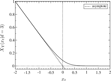
Refer to caption
Figure 2: The scaling function XΥ​(xt)X_{\Upsilon}(x_{t}) of the helicity modulus Υ⁡(T,L)\Upsilon(T,L) for d=3d=3. One observes that it is a monotonically decreasing function of xtx_{t}. The asymptote of XΥ​(xt)X_{\Upsilon}(x_{t}) for xt≪−1x_{t}\ll-1 is given in Eq. (95).

Let us determine the critical value of the finite-size helicity modulus Υ(βc,N⟂|d=3,𝒃)\Upsilon(\beta_{c},N_{\perp}|d=3,{\bm{b}}). Knowing the Casimir amplitude for antiperiodic boundary conditions ΔCasimir\Delta_{\rm Casimir} (see Eq. (81)) and that one under periodic boundary conditions [7] (see also [19])

ΔCasimirper=−25​π​ζ​(3)≃−0.153051,\Delta_{\rm Casimir}^{\rm per}=-\frac{2}{5\pi}\zeta(3)\simeq-0.153051, (93)

from Eq. (83) one obtains

βcΥ(βc,N⟂|d=3,𝒃)\displaystyle\beta_{c}\Upsilon(\beta_{c},N_{\perp}|d=3,{\bm{b}}) (94)
=\displaystyle= 2π2​N⟂​(J⟂J∥)​[ΔCasimir−ΔCasimirper]\displaystyle\frac{2}{\pi^{2}N_{\perp}}\left(\frac{J_{\perp}}{J_{\parallel}}\right)\left[\Delta_{\rm Casimir}-\Delta_{\rm Casimir}^{\rm per}\right]
=\displaystyle= 2π2​N⟂​(J⟂J∥)​[13​Cl2​(π3)+730​π​ζ​(3)]\displaystyle\frac{2}{\pi^{2}N_{\perp}}\left(\frac{J_{\perp}}{J_{\parallel}}\right)\left[\frac{1}{3}{\rm Cl}_{2}\left(\frac{\pi}{3}\right)+\frac{7}{30\pi}\zeta(3)\right]
≃\displaystyle\simeq 0.086649​N⟂−1​(J⟂J∥).\displaystyle 0.086649\;N_{\perp}^{-1}\left(\frac{J_{\perp}}{J_{\parallel}}\right).

Taking into account the relation ϱ⁡(Tc,L)=(m/ℏ)2​Υ​(T,L)\varrho(T_{c},L)=(m/\hbar)^{2}\Upsilon(T,L) between the superfluid density fraction and the helicity modulus (strictly speaking this is valid only for n=2n=2) one can obtain, within our model, an estimation of ϱ⁡(Tc,L)\varrho(T_{c},L) at TcT_{c}.

The dependence of the scaling function XΥ​(xt)X_{\Upsilon}(x_{t}) is shown in Fig. 2. It is easy to show that XΥ​(xt)X_{\Upsilon}(x_{t}) decays exponentially fast for xt≫1x_{t}\gg 1, while for xt≪−1x_{t}\ll-1 one derives that

XΥ(xt)≈xt→−∞−xt/2.X_{\Upsilon}(x_{t})\mathop{\approx}_{x_{t}\to-\infty}-x_{t}/2. (95)

The asymptote of XΥX_{\Upsilon} for T<TcT<T_{c} leads to Eq. (89) for the behavior of the helicity modulus within the anisotropic O⁡(n)O(n) models when n→∞n\to\infty in the limit limN⟂→∞βΥ(β,N⟂|d=3,𝒃)\lim_{N_{\perp}\to\infty}\beta\Upsilon(\beta,N_{\perp}|d=3,{\bm{b}}).

V Discussion and concluding remarks

Refer to caption
Figure 3: The scaling functions XCasimir​(xt)X_{\rm Casimir}(x_{t}) of the Casimir forces FCasimir(a)(β,N⟂|d=3,𝒃)F^{(a)}_{\rm Casimir}(\beta,N_{\perp}|d=3,{\bm{b}}) and FCasimir(p)(β,N⟂|d=3,𝒃)F^{(p)}_{\rm Casimir}(\beta,N_{\perp}|d=3,{\bm{b}}) for d=3d=3. The difference is due to the contributions stemming from the helicity modulus. We see that this contribution is rather strong and dominates the behavior of the force under antiperiodic boundary conditions converting it from attractive (under periodic boundary condition) into a repulsive one (under antiperiodic boundary conditions).

In the current article we studied the behavior of the Casimir force and the helicity modulus in anisotropic system with a diffuse interface as a function of the temperature. The interaction along the film is characterized via a coupling constant J∥J_{\parallel} while in the perpendicular to the film direction it is J⟂J_{\perp}. We have found that all scaling functions, including the Casimir amplitudes, depend on the ration J⟂/J∥J_{\perp}/J_{\parallel} and are, thus, nonuniversal. More precisely, we have found that the Casimir force in a dd-dimensional system, with 2<d<42<d<4, can be written in the form, see Eq. (69)

FCasimir(a)(T,N⟂|d,J⟂,J∥)\displaystyle F^{(a)}_{\rm Casimir}(T,N_{\perp}|d,J_{\perp},J_{\parallel}) (96)
=\displaystyle= (kB​Tc)​N⟂−d​XCasimir​(xt|d,J⟂,J∥),\displaystyle(k_{B}T_{c})\;N_{\perp}^{-d}\;X_{\rm Casimir}(x_{t}|d,J_{\perp},J_{\parallel}),

near the corresponding bulk critical temperature TcT_{c}, where xtx_{t} is a properly defined temperature dependent scaling variable and the nonuniversal scaling function

XCasimir​(xt|d,J⟂,J∥)=(J⟂J∥)(d−1)/2​XCasimir​(xt|d)X_{\rm Casimir}(x_{t}|d,J_{\perp},J_{\parallel})=\left(\frac{J_{\perp}}{J_{\parallel}}\right)^{(d-1)/2}X_{\rm Casimir}(x_{t}|d) (97)

can be related to XCasimir​(xt|d)X_{\rm Casimir}(x_{t}|d), which is the universal scaling function characterizing the corresponding isotropic system. The explicit form of XCasimir​(xt|d)X_{\rm Casimir}(x_{t}|d), for 2<d<42<d<4, is given in Eq. (63) and, equivalently, in (65). Similar relations can be written also for the helicity modulus, see Eq. (87)

Υ(T,N⟂|d,J⟂,J∥)=(kBTc)N⟂−(d−2)XΥ(xt|d,J⟂,J∥),\Upsilon(T,N_{\perp}|d,J_{\perp},J_{\parallel})=(k_{B}T_{c})\;N_{\perp}^{-(d-2)}\;X_{\Upsilon}(x_{t}|d,J_{\perp},J_{\parallel}), (98)

where, again, the nonuniversal scaling function XΥ​(xt|d,J⟂,J∥)X_{\Upsilon}(x_{t}|d,J_{\perp},J_{\parallel})

XΥ​(xt|d,J⟂,J∥)=(J⟂J∥)(d−1)/2​XΥ​(xt|d)X_{\Upsilon}(x_{t}|d,J_{\perp},J_{\parallel})=\left(\frac{J_{\perp}}{J_{\parallel}}\right)^{(d-1)/2}X_{\Upsilon}(x_{t}|d) (99)

can be related to universal scaling function XΥ​(xt|d)X_{\Upsilon}(x_{t}|d) characterizing the corresponding isotropic system. The explicit form of XΥ​(xt|d)X_{\Upsilon}(x_{t}|d), for 2<d<42<d<4, is given in Eq. (88).

From. Eq. (97) one obtains, see Eq. (70), that

ΔCasimir​(d|J⟂,J∥)=(J⟂J∥)(d−1)/2​ΔCasimir​(d).\Delta_{\rm Casimir}(d|J_{\perp},J_{\parallel})=\left(\frac{J_{\perp}}{J_{\parallel}}\right)^{(d-1)/2}\Delta_{\rm Casimir}(d). (100)

Since, within the spherical model, see Eq. (71),

ξ⟂ξ∥=J⟂J∥\frac{\xi_{\perp}}{\xi_{\parallel}}=\sqrt{\frac{J_{\perp}}{J_{\parallel}}} (101)

all the relations (97), (99) and (100) are in full conformity with our general prediction given by Eqs. (13) and (14) which relate quantities of one anisotropic system to the corresponding ones in the isotropic system.

In addition to general expressions pertinent to the case 2<d<42<d<4, we have also derived explicit results for the case d=3d=3. The scaling function of the Casimir force is given in Eq. (72) and, equivalently, in Eq. (73). The behavior of this function is visualized in Fig. 1. The scaling function for the helicity modulus is presented in Eq. (90) and is depicted in Fig. 2. For the value of the Casimir amplitude at d=3d=3 one has, see Eq. (81) [45],

ΔCasimir=[13​Cl2​(π3)−ζ⁡(3)6​π]​(J⟂J∥),\Delta_{\rm Casimir}=\left[\frac{1}{3}{\rm Cl}_{2}\left(\frac{\pi}{3}\right)-\frac{\zeta(3)}{6\pi}\right]\left(\frac{J_{\perp}}{J_{\parallel}}\right), (102)

while the value of the helicity modulus at TcT_{c} is, see Eq. (94),

βc​Υ​(Tc,L)=2π2​[13​Cl2​(π3)+7​ζ​(3)30​π]​(J⟂J∥)​L−1.\beta_{c}\Upsilon(T_{c},L)=\frac{2}{\pi^{2}}\left[\frac{1}{3}{\rm Cl}_{2}\Big(\frac{\pi}{3}\Big)+\frac{7\zeta(3)}{30\pi}\right]\left(\frac{J_{\perp}}{J_{\parallel}}\right)L^{-1}. (103)

Let us note that both the Casimir amplitude, as well as the Casimir force are positive, i.e. they correspond to a repulsion between the plates of the system. Let us stress that this effect is solely due to the existence of a diffuse interface in the system. We recall that under periodic boundary conditions for d=3d=3 and in the notations of the current article the Casimir force under periodic boundary conditions is given by the expression [17]

βFCasimir(p)(β,N⟂|d=3,𝒃)\displaystyle\beta F^{(p)}_{\rm Casimir}(\beta,N_{\perp}|d=3,{\bm{b}}) (104)
=\displaystyle= N⟂−3(b⟂b∥){14xt(yp−yb)−16​π(yp3/2−yb3/2)\displaystyle N_{\perp}^{-3}\left(\frac{b_{\perp}}{b_{\parallel}}\right)\Bigg\{\frac{1}{4}x_{t}(y_{p}-y_{b})-\frac{1}{6\pi}\left(y_{p}^{3/2}-y_{b}^{3/2}\right)
−ypπLi2(e−yp)−1πLi3(e−yp)}.\displaystyle-\frac{\sqrt{y_{p}}}{\pi}\text{Li}_{2}\left(e^{-\sqrt{y_{p}}}\right)-\frac{1}{\pi}\text{Li}_{3}\left(e^{-\sqrt{y_{p}}}\,\right)\Bigg\}.

The comparison between the force under antiperiodic and periodic boundary conditions is shown in Fig. 3. We observe that the contribution of the helicity energy is so strong that the Casimir force converts from being everywhere attractive (under periodic boundary conditions) into everywhere repulsive (under antiperiodic boundary conditions). This idea can eventually be used for practical purposes when applying some ordering external field might cause the border spins, dipoles, etc. to order in parallel or in antiparallel way to each other. Of course, by changing the degree of helicity the force will pass from being attractive through being zero into being repulsive. Obviously, it will be interesting to consider such a scenario in more details by say, studying a system under twisted at a given angle boundary conditions. We hope to return to this problem in a future work.

Acknowledgements.
D. D. would like to thank H.W. Diehl’s group and Fachbereich Physik of the Universität Duisburg-Essen for their hospitality at Campus Duisburg. We gratefully acknowledge the financial support of this work by the Deutsche Forschungsgemeinschaft via Grant No. Di-378/5, and the Bulgarian NSF (Project F-1402).

Appendix A Evaluation of U(w,N⟂|d,𝒃)U\left(w,N_{\perp}|d,{\bm{b}}\right)

In the current appendix we prove the validity of Eq. (III.1) for the behavior of U(w,N⟂|d,𝒃)U\left(w,N_{\perp}|d,{\bm{b}}\right) when N⟂≫1N_{\perp}\gg 1 and 0≤w≪10\leq w\ll 1. Because of the representation (37) of U(w,N⟂|d,𝒃)U\left(w,N_{\perp}|d,{\bm{b}}\right) and the asymptotes (III.1) of SN(a)​(x)S_{N}^{\rm(a)}(x) one divides the region of integration in two subregions - from 00 to a​N⟂2aN_{\perp}^{2} and from a​N⟂2aN_{\perp}^{2} to infinity, where aa is a fixed real number such that 0<a<10<a<1. Let us denote the integral over the first region (over ”moderate” values of xx) by UmU_{m} and let UlU_{l} is the integral over the ”large” values of xx, i.e. let

Um\displaystyle U_{m} ≡\displaystyle\equiv 12∫0a​N⟂2d​xx{exp(−x)−exp{−x[w−b⟂(1−cosπN⟂)]}[e−x​b⟂I0(xb⟂)+2π​x​b⟂R(−)(2​N⟂2x​b⟂)]×\displaystyle\frac{1}{2}\int_{0}^{aN_{\perp}^{2}}\frac{dx}{x}\Bigg\{\exp(-x)-\exp\left\{-x\left[w-b_{\perp}\left(1-\cos\frac{\pi}{N_{\perp}}\right)\right]\right\}\left[e^{-xb_{\perp}}I_{0}(xb_{\perp})+\sqrt{\frac{2}{\pi xb_{\perp}}}\;R^{\rm(-)}\left(\frac{2N_{\perp}^{2}}{xb_{\perp}}\right)\right]\times (105)
×[e−x​b∥I0(xb∥)]d−1}\displaystyle\times\left[e^{-xb_{\parallel}}I_{0}(xb_{\parallel})\right]^{d-1}\Bigg\}

and

Ul\displaystyle U_{l} ≡\displaystyle\equiv 12∫a​N⟂2∞d​xx{e−x−e−x​w[e−x​b∥I0(xb∥)]d−1×\displaystyle\frac{1}{2}\int_{aN_{\perp}^{2}}^{\infty}\frac{dx}{x}\Bigg\{e^{-x}-e^{-xw}\left[e^{-xb_{\parallel}}I_{0}(xb_{\parallel})\right]^{d-1}\times (106)
×[2N⟂+2N⟂R(+)(π2​b⟂2​N⟂2x)]}.\displaystyle\times\left[\frac{2}{N_{\perp}}+\frac{2}{N_{\perp}}R^{\rm(+)}\left(\frac{\pi^{2}b_{\perp}}{2N_{\perp}^{2}}x\right)\right]\Bigg\}.

Obviously U=Ul+UmU=U_{l}+U_{m}. The evaluation of UlU_{l} is straightforward. Since x≫1x\gg 1 in calculating UlU_{l} one can use the large value asymptote of the Bessel function [42]

Iν​(x)=exp⁡(x−ν2/2​x)2​π​x​[1+18​x+9−32​ν22!​(8​x)2+⋯]I_{\nu}(x)=\frac{\exp(x-\nu^{2}/2x)}{\sqrt{2\pi x}}\left[1+\frac{1}{8x}+\frac{9-32\nu^{2}}{2!(8x)^{2}}+\ \cdots\right] (107)

with the help of which one directly obtains that

Ul\displaystyle U_{l} =\displaystyle= −N⟂−d(b⟂b∥)(d−1)/21(4​π)(d−1)/2×\displaystyle-N_{\perp}^{-d}\left(\frac{b_{\perp}}{b_{\parallel}}\right)^{(d-1)/2}\frac{1}{(4\pi)^{(d-1)/2}}\times (108)
×∫a​b⟂/2∞d​xxx−(d−1)/2e−y​x[1+R(+)(π2x)],\displaystyle\times\int_{ab_{\perp}/2}^{\infty}\frac{dx}{x}x^{-(d-1)/2}e^{-yx}\left[1+R^{\rm(+)}\left(\pi^{2}x\right)\right],\qquad

where yy is defined in Eq. (49). Let us deal now with the term UmU_{m}. We divide this term into ”bulk-like” contributions Um,bU_{\rm m,b} and ”finite-size” contributions Um,fsU_{\rm m,fs} where Um=Um,b+Um,fsU_{m}=U_{\rm m,b}+U_{\rm m,fs} with

Um,b\displaystyle U_{\rm m,b} ≡\displaystyle\equiv 12∫0a​N⟂2d​xx{e−x−e−x​w~[e−x​b⟂I0(xb⟂)]×\displaystyle\frac{1}{2}\int_{0}^{aN_{\perp}^{2}}\frac{dx}{x}\Big\{e^{-x}-e^{-x\tilde{w}}\left[e^{-xb_{\perp}}I_{0}(xb_{\perp})\right]\times (109)
×[e−x​b∥I0(xb∥)]d−1}\displaystyle\times\left[e^{-xb_{\parallel}}I_{0}(xb_{\parallel})\right]^{d-1}\Big\}

and

Um,fs\displaystyle U_{\rm m,fs} ≡\displaystyle\equiv −∫0a​N⟂2d​xxe−x​w~12​π​x​b⟂R(−)(2​N⟂2x​b⟂)×\displaystyle-\int_{0}^{aN_{\perp}^{2}}\frac{dx}{x}e^{-x\tilde{w}}\frac{1}{\sqrt{2\pi xb_{\perp}}}\;R^{\rm(-)}\left(\frac{2N_{\perp}^{2}}{xb_{\perp}}\right)\times (110)
×[e−x​b∥​I0​(x​b∥)]d−1,\displaystyle\times\left[e^{-xb_{\parallel}}I_{0}(xb_{\parallel})\right]^{d-1},

where

w~=w−b⟂​(1−cos⁡πN⟂).\tilde{w}=w-b_{\perp}\left(1-\cos\frac{\pi}{N_{\perp}}\right). (111)

It is straightforward to evaluate Um,fsU_{\rm m,fs}. Due to the representation (46), for all x≪N⟂2x\ll N_{\perp}^{2} the corresponding contribution into the integral on the right-hand side of Eq. (110) will be exponentially small. Thus, one again can use in (110) the large-value asymptote (107) of the Bessel function I0​(x)I_{0}(x) which leads to

Um,fs\displaystyle U_{\rm m,fs} =\displaystyle= −N⟂−d(b⟂b∥)(d−1)/21(4​π)d/2×\displaystyle-N_{\perp}^{-d}\left(\frac{b_{\perp}}{b_{\parallel}}\right)^{(d-1)/2}\frac{1}{(4\pi)^{d/2}}\times (112)
×∫0a​b⟂/2d​xxx−d/2e−y~​xR(−)(1x).\displaystyle\times\int_{0}^{ab_{\perp}/2}\frac{dx}{x}x^{-d/2}e^{-\tilde{y}x}R^{\rm(-)}\left(\frac{1}{x}\right).

It remains now only to deal with the term Um,bU_{\rm m,b}. By subtracting and adding, up to the linear in xx term, the asymptote of exp⁡[x​b⟂​(1−cos⁡πN⟂)]\exp\left[xb_{\perp}\left(1-\cos\frac{\pi}{N_{\perp}}\right)\right] for small values of xx one rewrites Eq. (109) into the form

Um,b\displaystyle U_{\rm m,b} =\displaystyle= 12∫0a​N⟂2d​xx{e−x−(1+12b⟂π2N⟂2x)e−x​w\displaystyle\frac{1}{2}\int_{0}^{aN_{\perp}^{2}}\frac{dx}{x}\Bigg\{e^{-x}-\left(1+\frac{1}{2}b_{\perp}\frac{\pi^{2}}{N_{\perp}^{2}}x\right)e^{-xw} (113)
×[e−x​b⟂I0(xb⟂)][e−x​b∥I0(xb∥)]d−1}\displaystyle\times\left[e^{-xb_{\perp}}I_{0}(xb_{\perp})\right]\left[e^{-xb_{\parallel}}I_{0}(xb_{\parallel})\right]^{d-1}\Bigg\}
+12∫0a​N⟂2d​xx[(1+12b⟂π2N⟂2x)e−x​w−e−x​w~]\displaystyle+\frac{1}{2}\int_{0}^{aN_{\perp}^{2}}\frac{dx}{x}\left[\left(1+\frac{1}{2}b_{\perp}\frac{\pi^{2}}{N_{\perp}^{2}}x\right)e^{-xw}-e^{-x\tilde{w}}\right]
×[e−x​b⟂​I0​(x​b⟂)]​[e−x​b∥​I0​(x​b∥)]d−1.\displaystyle\times\left[e^{-xb_{\perp}}I_{0}(xb_{\perp})\right]\left[e^{-xb_{\parallel}}I_{0}(xb_{\parallel})\right]^{d-1}.

It is easy to understand that the integration over small values of xx in the second line of the above equation will provide contributions of the order of O⁡(N⟂−4)O(N_{\perp}^{-4}) which we will neglect, since we are only interested in contributions that are not smaller than O⁡(N⟂−d)O(N_{\perp}^{-d}), with 2<d<42<d<4. Thus, in this integral one again can use the large value asymptote (107) of the Bessel function I0​(x)I_{0}(x), which leads to

Um,b\displaystyle U_{\rm m,b} =\displaystyle= 12∫0a​N⟂2d​xx{e−x−e−x​w[e−x​b⟂I0(xb⟂)][e−x​b∥I0(xb∥)]d−1}−14b⟂π2N⟂2∫0a​N⟂2dxe−x​w[e−x​b⟂I0(xb⟂)]×\displaystyle\frac{1}{2}\int_{0}^{aN_{\perp}^{2}}\frac{dx}{x}\Bigg\{e^{-x}-e^{-xw}\left[e^{-xb_{\perp}}I_{0}(xb_{\perp})\right]\left[e^{-xb_{\parallel}}I_{0}(xb_{\parallel})\right]^{d-1}\Bigg\}-\frac{1}{4}b_{\perp}\frac{\pi^{2}}{N_{\perp}^{2}}\int_{0}^{aN_{\perp}^{2}}dx\;e^{-xw}\left[e^{-xb_{\perp}}I_{0}(xb_{\perp})\right]\times (114)
×[e−x​b∥I0(xb∥)]d−1+N⟂−d(b⟂b∥)(d−1)/2121(4​π)d/2∫0a​b⟂/2d​xx[e−x​y(1+π2x)−e−x​y~]x−d/2.\displaystyle\times\left[e^{-xb_{\parallel}}I_{0}(xb_{\parallel})\right]^{d-1}+N_{\perp}^{-d}\left(\frac{b_{\perp}}{b_{\parallel}}\right)^{(d-1)/2}\frac{1}{2}\frac{1}{(4\pi)^{d/2}}\int_{0}^{ab_{\perp}/2}\frac{dx}{x}\left[e^{-xy}\left(1+\pi^{2}x\right)-e^{-x\tilde{y}}\;\right]x^{-d/2}.

One can complete the integral in the first and second line of the above equation so that the integration is from 00 to ∞\infty and to subtract the parts of integration from a​N⟂2aN_{\perp}^{2} to ∞\infty. In the subtracted parts one can again use the large value asymptote (107) of the Bessel function I0​(x)I_{0}(x). In this way one obtains

Um,b\displaystyle U_{\rm m,b} = U_d(w—b)- 1 4 b_⟂ π 2 N ⟂ 2 W_d(w—b)+N_⟂^-d( b ⟂ b ∥ )^(d-1)/2 1 2 1 (4π) d/2 [∫_a b_⟂/2^∞ dx x  e^-x y(1+π^2 x) x^-d/2
+∫0a​b⟂/2d​xx[e−x​y(1+π2x)−e−x​y~]x−d/2].\displaystyle+\int_{0}^{ab_{\perp}/2}\frac{dx}{x}\left[e^{-xy}\left(1+\pi^{2}x\right)-e^{-x\tilde{y}}\;\right]x^{-d/2}\Bigg].

Expressing from Eq. (59) function R(−)​(x)R^{\rm(-)}(x) in terms of R(+)​(x)R^{\rm(+)}(x) and substituting the so-obtained representation in Eq. (112) one obtains

Um,fs\displaystyle U_{\rm m,fs} =\displaystyle= −N⟂−d(b⟂b∥)(d−1)/21(4​π)(d−1)/2∫0a​b⟂/2d​xxx−(d−1)/2e−y​x[1+R(+)(π2x)−1214​π​xeπ2​x]\displaystyle-N_{\perp}^{-d}\left(\frac{b_{\perp}}{b_{\parallel}}\right)^{(d-1)/2}\frac{1}{(4\pi)^{(d-1)/2}}\int_{0}^{ab_{\perp}/2}\frac{dx}{x}x^{-(d-1)/2}e^{-yx}\left[1+R^{\rm(+)}\left(\pi^{2}x\right)-\frac{1}{2}\frac{1}{\sqrt{4\pi x}}e^{\pi^{2}x}\right] (116)
=\displaystyle= −N⟂−d(b⟂b∥)(d−1)/21(4​π)(d−1)/2{∫0a​b⟂/2d​xxx−(d−1)/2e−y​x[1+R(+)(π2x)−1214​π​x(1+π2x)]\displaystyle-N_{\perp}^{-d}\left(\frac{b_{\perp}}{b_{\parallel}}\right)^{(d-1)/2}\frac{1}{(4\pi)^{(d-1)/2}}\Bigg\{\int_{0}^{ab_{\perp}/2}\frac{dx}{x}x^{-(d-1)/2}e^{-yx}\left[1+R^{\rm(+)}\left(\pi^{2}x\right)-\frac{1}{2}\frac{1}{\sqrt{4\pi x}}\left(1+\pi^{2}x\right)\right]
+1214​π∫0a​b⟂/2d​xxx−d/2e−y​x[(1+π2x)−eπ2​x]}.\displaystyle+\frac{1}{2}\frac{1}{\sqrt{4\pi}}\int_{0}^{ab_{\perp}/2}\frac{dx}{x}x^{-d/2}e^{-yx}\left[\left(1+\pi^{2}x\right)-e^{\pi^{2}x}\right]\Bigg\}.

In a similar way, by adding and subtracting the asymptote of 1+R(+)​(π2​x)1+R^{\rm(+)}\left(\pi^{2}x\right) for small values of the arument, one can rewrite UlU_{l} (see Eq. (108)) into the form

Ul\displaystyle U_{l} =\displaystyle= −N⟂−d(b⟂b∥)(d−1)/21(4​π)(d−1)/2{∫a​b⟂/2∞d​xxx−(d−1)/2e−y​x[1+R(+)(π2x)−1214​π​x(1+π2x)]\displaystyle-N_{\perp}^{-d}\left(\frac{b_{\perp}}{b_{\parallel}}\right)^{(d-1)/2}\frac{1}{(4\pi)^{(d-1)/2}}\Bigg\{\int_{ab_{\perp}/2}^{\infty}\frac{dx}{x}x^{-(d-1)/2}e^{-yx}\left[1+R^{\rm(+)}\left(\pi^{2}x\right)-\frac{1}{2}\frac{1}{\sqrt{4\pi x}}\left(1+\pi^{2}x\right)\right] (117)
+1214​π∫0a​b⟂/2d​xxx−d/2e−y​x(1+π2x)}.\displaystyle+\frac{1}{2}\frac{1}{\sqrt{4\pi}}\int_{0}^{ab_{\perp}/2}\frac{dx}{x}x^{-d/2}e^{-yx}\left(1+\pi^{2}x\right)\Bigg\}.

By adding Um,bU_{\rm m,b}, Um,fsU_{\rm m,fs}, and UlU_{l} as given by Eqs. (A), (116) and (117), respectively, one obtains, after using the representation (51) for Ud​(w|𝒃)U_{d}(w|\bm{b}), as well as the fact that Wd​(w|𝒃)=∂Ud​(w|𝒃)/∂ωW_{d}(w|\bm{b})=\partial U_{d}(w|\bm{b})/\partial\omega, the final result for U(w,N⟂|d,𝒃)U\left(w,N_{\perp}|d,{\bm{b}}\right) given in Eq. (III.1) in the main text.

Appendix B Derivation of the series representation of I⁡(y,d)I(y,d)

In this appendix we derive the power series representation (61) of the integral I⁡(y,d)I(y,d) defined in Eq. (58).

First, let us note that using the representation (42) for the function R(+)​(x)R^{\rm(+)}(x), the integral I⁡(y,d)I(y,d) can be decomposed as I⁡(y,d)=I[1]​(y,d)+I[2]​(y,d)I(y,d)=I^{[1]}(y,d)+I^{[2]}(y,d), where

I[1]​(y,d)\displaystyle I^{[1]}(y,d) =\displaystyle= −1(4​π)(d−1)/2×\displaystyle-\frac{1}{(4\pi)^{(d-1)/2}}\times
×∑n=1∞∫0∞dxx−(d+1)/2e−y​xe−4​π2​n​(n+1)​x\displaystyle\times\sum_{n=1}^{\infty}\int_{0}^{\infty}dx\,x^{-(d+1)/2}e^{-yx}e^{-4\pi^{2}n(n+1)x}\quad

and

I[2]​(y,d)\displaystyle I^{[2]}(y,d) =\displaystyle= −1(4​π)(d−1)/2×\displaystyle-\frac{1}{(4\pi)^{(d-1)/2}}\times
×∫0∞dxx−(d+1)/2e−y​x[1−1+π2​x2​4​π​x].\displaystyle\times\int_{0}^{\infty}dx\,x^{-(d+1)/2}e^{-yx}\!\left[1-\frac{1+\pi^{2}x}{2\sqrt{4\pi x}}\right].\quad

Employing dimensional regularization, the latter integral can be done analytically and becomes

I[2]​(y,d)\displaystyle I^{[2]}(y,d) =\displaystyle= y(d−2)/22​(4​π)d/2{π2Γ(1−d/2)\displaystyle\frac{y^{(d-2)/2}}{2(4\pi)^{d/2}}\!\Big\{\pi^{2}\,\Gamma\left(1-d/2\right) (120)
−4π​yΓ[(1−d)/2]+yΓ(−d/2)}.\displaystyle-4\sqrt{\pi y}\Gamma\left[(1-d)/2\right]+y\,\Gamma\left(-d/2\right)\Big\}.

Introducing the variable y~≡y−π2\tilde{y}\equiv y-\pi^{2}, the integral I[1]​(y,d)I^{[1]}(y,d) can be written as

I[1]​(y,d)\displaystyle I^{[1]}(y,d) =\displaystyle= −1(4​π)(d−1)/2×\displaystyle-\frac{1}{(4\pi)^{(d-1)/2}}\times
×∑n=1∞∫0∞d​xx(d+1)/2​e−y~​x​e−[π2+4​π2​n​(n+1)]​x\displaystyle\times\sum_{n=1}^{\infty}\int_{0}^{\infty}\frac{dx}{x^{(d+1)/2}}e^{-\tilde{y}x}e^{-[\pi^{2}+4\pi^{2}n(n+1)]x}

and upon replacing exp⁡(−y~​x)\exp(-\tilde{y}x) by its Taylor series representation the integral I[1]​(y,d)I^{[1]}(y,d) becomes

I[1](y,d)=−1(4​π)(d−1)/2∑n=1∞∑m=0∞bn,m(d)(−y~)mm!.I^{[1]}(y,d)=-\frac{1}{(4\pi)^{(d-1)/2}}\sum_{n=1}^{\infty}\sum_{m=0}^{\infty}b^{(d)}_{n,m}\frac{(-\tilde{y})^{m}}{m!}. (122)

with the coefficients

bn,m(d)​(y)=∫0∞d​x​xm−(d+1)/2​e−[π2+4​π2​n​(n+1)]​x.b^{(d)}_{n,m}(y)=\int_{0}^{\infty}dx\,x^{m-(d+1)/2}e^{-[\pi^{2}+4\pi^{2}n(n+1)]x}. (123)

Again in the sense of dimensional regularization the xx-integration in the latter equation can be performed to give

bn,m(d)​(y)=(n+12)d−2​m−1​Γ​(m+1−d2)(2​π)2​m+1−d.b^{(d)}_{n,m}(y)=\frac{\left(n+\frac{1}{2}\right)^{d-2m-1}\Gamma\!\left(m+\frac{1-d}{2}\right)}{(2\pi)^{2m+1-d}}. (124)

Inserting this into Eq. (122), the nn-summation can be done analytically leading to

I[1]​(y,d)\displaystyle I^{[1]}(y,d) =\displaystyle= π(d−1)/2[21−d∑m=0∞(−y~)m​Γ​(m+1−d2)π2​m​m!\displaystyle\pi^{(d-1)/2}\Bigg[2^{1-d}\sum_{m=0}^{\infty}\frac{(-\tilde{y})^{m}\Gamma\!\left(m+\frac{1-d}{2}\right)}{\pi^{2m}m!} (125)
−∑m=0∞am(d)(−y~)m]\displaystyle-\sum_{m=0}^{\infty}a^{(d)}_{m}(-\tilde{y})^{m}\Bigg]

with the coefficients am(d)a^{(d)}_{m} defined in Eq. (62). The first mm-sum in square brackets can also be done analytically and we obtain

I[1]​(y,d)\displaystyle I^{[1]}(y,d) =\displaystyle= (4​π)(1−d)/2​Γ​[(1−d)/2]​(y~+π2)(d−1)/2\displaystyle(4\pi)^{(1-d)/2}\Gamma\left[(1-d)/2\right](\tilde{y}+\pi^{2})^{(d-1)/2} (126)
−π(d−1)/2∑m=0∞am(d)(−y~)m.\displaystyle-\pi^{(d-1)/2}\sum_{m=0}^{\infty}a^{(d)}_{m}(-\tilde{y})^{m}.

If we now add up I[1]​(y,d)I^{[1]}(y,d) and I[2]​(y,d)I^{[2]}(y,d) we arrive at the power series representation (61) of I⁡(y,d)I(y,d) given in the main text. Note that no terms being nonanalytic with respect to y~\tilde{y} are present, and furthermore that the radius of convergence of the expansion is |y~|=|y−π2|<4​π2|\tilde{y}|=|y-\pi^{2}|<4\pi^{2}.

References

  • [1] H. B. G. Casimir, Proc. K. Ned. Akad. Wet. 51, 793 (1948).
  • [2] M. E. Fisher and P. G. de Gennes, C. R. Acad. Sc. Paris B 287, 207 (1978).
  • [3] R. Evans, in Liquids at interfaces, Les Houches Session XLVIII, edited by J. Charvolin, J. Joanny and J. Zinn-Justin (Elsevier, Amsterdam, 1990), p. 3.
  • [4] M. Krech, The Casimir Effect in Critical Systems (World Scientific, Singapore, 1994).
  • [5] J. G. Brankov, D. M. Danchev, and N. S. Tonchev, The Theory of Critical Phenomena in Finite-Size Systems - Scaling and Quantum Effects (World Scientific, Singapore, 2000).
  • [6] M. Krech and S. Dietrich, Phys. Rev. Lett. 66, 345 (1991); Phys. Rev. A 46, 1886 (1992); ibid 46, 1922 (1992), and references therein.
  • [7] D.M. Danchev, Phys. Rev. E 53, 2104 (1996); ibid 58, 1455 (1998).
  • [8] M. Krech, Phys. Rev. E 56, 1642 (1997).
  • [9] M. Krech, J. Phys.: Condens. Matter 11, R391 (1999).
  • [10] R. Garcia and M. H. W. Chan, Phys. Rev. Lett. 83, 1187 (1999); Physica B 280, 55 (2000); J. Low Temp. Phys. 121, 495 (2000).
  • [11] R. Garcia and M. H. W. Chan, Phys. Rev. Lett. 88, 086101 (2002).
  • [12] A. Mukhopadhyay and B. M. Law, Phys. Rev. Lett. 83, 772 (1999); Phys. Rev. E. 62, 5201 (2000); ibid 63, 041605 (2001).
  • [13] T. Ueno, S. Balibar, T. Mizusaki, F. Caupin, and E. Rolley, Phys. Rev. Lett. 90, 116102 (2003); R. Ishiguro and S. Balibar, J. Low. Temp. Phys. 140, 29 (2005).
  • [14] A. Ganshin, S. Scheidemantel, R. Garcia, and M. H.W. Chan, Phys. Rev. Lett. 97, 075301 (2006).
  • [15] D. Dantchev, M. Krech, and S. Dietrich, Phys. Rev. E 67, 066120 (2003).
  • [16] F. Schlesener, A. Hanke, and S. Dietrich, J. Stat. Phys. 110, 981 (2003).
  • [17] D. Danchev and M. Krech, Phys. Rev. E 69, 046119 (2004).
  • [18] M. Fukuto, Y. F. Yano, and P. S. Pershan, Phys. Rev. Lett. 94, 135702 (2005).
  • [19] D. Dantchev, H. W. Diehl, D. Grüneberg, Phys. Rev. E 73, 016131 (2006).
  • [20] H. W. Diehl, D. Grüneberg, and M. A. Shpot, Europhys. Lett. 75, 241 (2006).
  • [21] D. Dantchev, F. Schlesener and S. Dietrich, Phys. Rev. E 76, 011121 (2007).
  • [22] O. Vasilyev, A. Gambassi, A. Maciolek, and S. Dietrich, Euro. Phys. Lett. 80, 60009 (2007).
  • [23] A. Hucht, Phys. Rev. Lett. 99, 185301 (2007).
  • [24] D. Grüneberg and H. W. Diehl, Phys. Rev. B 77, 115409 (2008).
  • [25] C. Hertlein, L. Helden, A. Gambassi, S. Dietrich, and C. Bechinger, Nature 451, 172 (2008).
  • [26] V. Privman, in Finite Size Scaling and Numerical Simulations of Statistical Systems, edited by V. Privman (World Scientific, Singapore, 1990).
  • [27] D. Danchev, J. Stat. Phys. 73, 267 (1993).
  • [28] V. Privman, J. Phys. A 23, L711 (1990).
  • [29] M. E. Fisher, M. N. Barber, and D. Jasnow, Phys. Rev. A 8, 111 (1973).
  • [30] I. Rhee, F. M. Gasparini, and D. J. Bishop, Phys. Rev. Lett. 63, 410 (1989).
  • [31] F. M. Gasparini and I. Rhee, in Progress in Low Temperature Physics, Vol. 6, D. F. Brewer, ed. (North-Holland, Amsterdam, 1991), Chapter I.
  • [32] X. S. Chen and V. Dohm, Phys. Rev. 70, 056136 (2004).
  • [33] V. Dohm, cond-mat arXiv:0801.4096v2.
  • [34] D. Stauffer, M. Ferer, and M. Wortis, Phys. Rev. Lett. 29, 345 (1972).
  • [35] A. Aharony, Phys. Rev. B 9, 2107 (1974).
  • [36] P.R. Gerber, J. Phys. A 8, 67 (1975).
  • [37] P.C. Hohenberg, A. Aharony, B.I. Halperin, and E.D. Siggia, Phys. Rev. B 13, 2986 (1976).
  • [38] F. Wegner, in Phase Transitions and Critical Phenomena, edited by C. Domb and M.S. Green (Academic, New York, 1976), Vol.6, p.7.
  • [39] V. Privman, A. Aharony, and P.C. Hohenberg, in Phase Transitions and Critical Phenomena, edited by C. Domb and J. L. Lebowitz (Academic, New York, 1991), Vol. 14, p. 1.
  • [40] V. Privman and M. E. Fisher, Phys. Rev. B 30, 322 (1984).
  • [41] S. Singh and R. K. Pathria, Phys. Rev. Lett. 55, 347 (1985).
  • [42] S. Singh and R. K. Pathria, Phys. Rev. B 85, 4618 (1985).
  • [43] The results presented in Eqs. (17) and (20) can also be considered as a generalization toward antiperiodic boundary conditions of the correspondingg results of [17] for the spherical model with anisotropic interaction and periodic boundary conditions.
  • [44] J. Choi and D. Cvijovic, J. Phys. A 40, 15019 (2007).
  • [45] The numerical value of ΔCasimir≃0.274543\Delta_{\rm Casimir}\simeq 0.274543 in the isotropic case has recently been also reported in H. Chamati, arXiv:0805.0715.