August 24, 2026
The Slice Algorithm For Irreducible Decomposition of Monomial Ideals
Abstract.
Irreducible decomposition of monomial ideals has an increasing number of applications from biology to pure math. This paper presents the Slice Algorithm for computing irreducible decompositions, Alexander duals and socles of monomial ideals. The paper includes experiments showing good performance in practice.
1. Introduction
The main contribution of this paper is the Slice Algorithm, which is an algorithm for the computation of the irreducible decomposition of monomial ideals. To irreducibly decompose an ideal is to write it as an irredundant intersection of irreducible ideals.
Irreducible decomposition of monomial ideals has an increasing number of applications from biology to pure math. Some examples of this are the Frobenius problem [1, 2], the integer programming gap [3], the reverse engineering of biochemical networks [4], tropical convex hulls [5], tropical cyclic polytopes [5], secants of monomial ideals [6], differential powers of monomial ideals [7] and joins of monomial ideals [6].
Irreducible decomposition of a monomial ideal has two computationally equivalent guises. The first is as the Alexander dual of [8], and indeed some of the references above are written exclusively in terms of Alexander duality rather than irreducible decomposition. The second is as the socle of the vector space , where is the polynomial ring that belongs to and for some integer . The socle is central to this paper, since what the Slice algorithm actually does is to compute a basis of the socle.
Section 2 introduces some basic notions we will need throughout the paper and Section 3 describes an as-simple-as-possible version of the Slice Algorithm. Section 3.4 contains improvements to this basic version of the algorithm and Section 5 discusses some heuristics that are inherent to the algorithm. Section 6 examines applications of irreducible decomposition, and it describes how the Slice Algorithm can use bounds to solve some optimization problems involving irreducible decomposition in less time than would be needed to actually compute the decomposition. Finally, Section 7 explores the practical aspects of the Slice Algorithm including benchmarks comparing it to other programs for irreducible decomposition.
2. Preliminaries
This section briefly covers some notation and background on monomial ideals that is necessary to read the paper. We assume throughout the paper that , and are monomial ideals in a polynomial ring over some arbitrary field and with variables where . We also assume that , , , and are monomials in . When presenting examples we use the variables , and in place of , and for increased readability.
2.1. Basic Notions From Monomial Ideals
If then . We define where . Define such that e.g. .
The rest of this section is completely standard. A monomial ideal is an ideal generated by monomials, and is the unique minimal set of monomial generators. The ideal is the ideal generated by the elements of the set . The colon ideal is defined as .
An ideal is artinian if there exists a such that for . A monomial of the form is a pure power. A monomial ideal is irreducible if it is generated by pure powers. Thus is irreducible while is not. Note that is irreducible and not artinian.
Every monomial ideal can be written as an irredundant intersection of irreducible monomial ideals, and the set of ideals that appear in this intersection is uniquely given by . This set is called the irreducible decomposition of , and we denote it by . Thus .
The radical of a monomial ideal is . A monomial ideal is square free if . A monomial ideal is (strongly) generic if no two distinct elements of raise the same variable to the same non-zero power [12, 13]. Thus is generic while is not as both minimal generators raise to the same power. In this paper we informally talk of a monomial ideal being more or less generic according to how many identical non-zero exponents there are in .
A standard monomial of is a monomial that does not lie within . The exponent vector of a monomial is defined by . Define . We draw pictures of monomial ideals in 2 and 3 dimensions by indicating monomials by their exponent vector and drawing line segments separating the standard monomials from the non-standard monomials. Thus Figure 1(a) displays a picture of the monomial ideal .
 |
 |
 |
| (a) | (b) | (c) |
2.2. Maximal Standard Monomials, Socles And Decompositions
In this section we look into socles and their relationship with irreducible decomposition. We also note the well known fact that the maximal standard monomials of form a basis of the socle of .
Given the generators of a monomial ideal , the Slice Algorithm computes the maximal standard monomials of . We will need some notation for this.
Definition 1 (Maximal standard monomial).
A monomial is a maximal standard monomial of if and for . The set of maximal standard monomials of is denoted by .
The socle of is the vector space of those such that for . It is immediate that is a basis of this socle.
Example 2.
We will briefly describe the standard technique for obtaining from [12]. Choose some integer and define .
Proposition 3 ([14, ex. 5.8]).
The map is a bijection from to .
Example 4.
Let and where . Then which maps to .
2.3. Labels
We will have frequent use for the notion of a label.
Definition 5 (-label).
Let be a standard monomial of and let . Then is an -label of if .
Note that if is an -label of , then . Also, a standard monomial is maximal if and only if it has an -label for . So in that case .
Example 6.
Let be the ideal in Figure 2(a). Then the maximal standard monomials of are . We see that has as an -label, as a -label and as a -label. Also, has as an -label and as a -label, while it has both of and as -labels.
Let be the ideal in Figure 2(b). Then . Note that even though divides , it is not a label of , because it does not divide , or .
 |
 |
| (a) | (b) |
3. The Slice Algorithm
In this section we describe a basic version of the Slice Algorithm. The Slice Algorithm computes the maximal standard monomials of a monomial ideal given the minimal generators of that ideal.
A fundamental idea behind the Slice Algorithm is to consider certain subsets of that are represented as slices. We will define the meaning of the term slice shortly. The algorithm starts out by considering a slice that represents all of . It then processes this slice by splitting it into two simpler slices. This process continues recursively until the slices are simple enough that it is easy to find any maximal standard monomials within them.
From this description, there are a number of details that need to be explained. Section 3.1 covers what slices are and how to split them while Section 3.2 covers the base case. Section 3.3 proves that the algorithm terminates and Section 3.4 contains a simple pseudo-code implementation of the algorithm.
3.1. Slices And Splitting
In this section we explain what slices are and how to split them. We start off with the formal definition of a slice and its content.
Definition 7 (Slice and content).
A slice is a 3-tuple where and are monomial ideals and is a monomial. The content of a slice is defined by .
Example 8 shows how this definition is used.
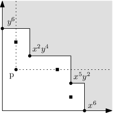 |
 |
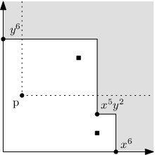 |
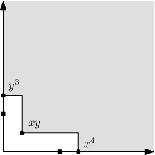
| (a) | (b) | (c) |
Example 8.
Let and . Then is the ideal depicted in Figure 3(a), where is indicated by the dotted line and is indicated by the squares. We will compute by performing a step of the Slice Algorithm.
Let be the ideal , as depicted in Figure 3(b), where is indicated by the squares. As can be seen by comparing figures 3(a) and 3(b), the ideal corresponds to the part of the ideal that lies within . Thus it is reasonable to expect that corresponds to the subset of that lies within , which turns out to be true, since
| (1) |
It now only remains to compute . Let as depicted in Figure 3(c), where is indicated by the squares. The dotted line indicates that we are ignoring everything inside . It happens to be that one of the minimal generators of , namely , lies in the interior of , which allows us to ignore that minimal generator. We are looking at because
| (2) |
By combining Equation (1) and Equation (2), we can compute in terms of , and .
Having defined slices and their content, we can now explain how to split a slice into two smaller slices. This is done by choosing some monomial , called the pivot, and then to consider the following trivial equation.
| (3) |
The idea is to express both parts of this disjoint union as the content of a slice. This is easy to do for the last part, since
Expressing the first part of the union as the content of a slice can be done using the following equation, which we will prove at the end of this section.
which implies that (see Example 8)
Thus we can turn Equation (3) into the following.
| (4) |
Equation (4) is the basic engine of the Slice Algorithm. We will refer to it and its parts throughout the paper, and we need some terminology to facilitate this. The process of applying Equation (4) is called a pivot split. We will abbreviate this to just split when doing so should not cause confusion.
Equation (4) mentions three slices, and we give each of them a name. We call the left hand slice the current slice, since it is the slice we are currently splitting. We call the first right hand slice the inner slice, since its content is inside , and we call the second right hand slice the outer slice, since its content is outside .
It is not immediately obvious why it is easier to compute the outer slice’s content than it is to compute the current slice’s content . The following equation shows how it can be easier. See Proposition 11 for a proof.
| (5) |
This implies that . In other words, we can discard any element of where lies within . We will apply Equation (5) whenever it is of benefit to do so, which it is when . This motivates the following definition.
Definition 9 (Normal slice).
A slice is normal when .
Example 10.
Proposition 11 proves the equations in this section, and it establishes some results that we will need later.
Proposition 11.
Let be a monomial ideal and let be a monomial. Then
- (1)
divides
- (2)
- (3)
If , then
- (4)
- (5)
Proof.
: Let . Let be an -label of and let be an -label of where . This is possible due to the assumption in Section 2 that . Then and so .
: If then by (1), whereby
: As and , we see that
: Let and let be an -label of . Then since . Thus since , so . Also .
Suppose instead that . Then . If then there would exist an such that , which is a contradiction since then . Thus whereby . ∎
Lemma 12.
Let , and be monomial ideals. Then implies that .
Proof.
Let . We will prove that .
: If then but .
: Follows from and since then . ∎
3.2. The Base Case
In this section we present the base case for the Slice Algorithm. A slice is a base case slice if is square free or if does not divide . Propositions 13 and 14 show why base case slices are easy to handle.
Proposition 13.
If does not divide , then .
Proof.
If then there exists some . Let be an -label of . Then , so . ∎
Proposition 14.
If is square free and , then .
Proof.
Let be square free and let . Let be an -label of for . Then so . ∎
3.3. Termination And Pivot Selection
In this section we show that some quite weak constraints on the choice of the pivot are sufficient to ensure termination. Thus we leave the door open for a variety of different pivot selection strategies, which is something we will have much more to say about in Section 5.
We impose four conditions on the choice of the pivot . These are presented below, and for each condition we explain why violating that condition would result in a split that there is no sense in carrying out. Note that the last two conditions are not necessary at this point to ensure termination, but they will become so after some of the improvements in Section 3.4 are applied.
- :
-
If , then the outer slice will be equal to the current slice.
- :
-
If , then the inner slice will be equal to the current slice.
- :
- :
If a pivot satisfies these four conditions, then we say that it is valid. Proposition 15 shows that non-base case slices always admit valid pivots, and Proposition 16 states that selecting valid pivots ensures termination.
Proposition 15.
Let be a normal slice for which no valid pivot exists. Then is square free.
Proof.
Suppose is not square free. Then there exists an such that for some , which implies that . Also, since and is normal. We conclude that is a valid pivot. ∎
Proposition 16.
Selecting valid pivots ensures termination.
Proof.
Recall that the polynomial ring is noetherian, so it does not contain an infinite sequence of strictly increasing ideals. We will use this to show that the algorithm terminates. Suppose we are splitting a non-base case slice on a valid pivot where is the inner slice and is the outer slice.
Let and be functions mapping slices to ideals, and define them by the expressions and . Then the conditions on valid pivots and on non-base case slices imply that , , and . Also, if we let be an arbitrary slice and we let be the corresponding normal slice, then and .
Thus and never decrease, and one of them strictly increases on the outer slice while the other strictly increases on the inner slice. Thus there does not exist an infinite sequence of splits on valid pivots. ∎
3.4. Pseudo-code
This section contains a pseudo-code implementation of the Slice Algorithm. Note that the improvements in Section 3.4 are necessary to achieve good performance.
The function selectPivot used below returns some valid pivot and can be implemented according to any of the pivot selection strategies presented in Section 5. A simple idea is to follow the proof of Proposition 15 and test each variable for whether it is a valid pivot. If none of those are valid pivots, then in the pseudo-code below is square free.
Call the function below with the parameters to obtain .
-
function con(, , )
-
let
-
if does not divide then return
-
if is square free and then return
-
if is square free and then return
-
let := selectPivot(, )
-
return
4. Improvements To The Basic Algorithm
This section contains a number of improvements to the basic version of the Slice Algorithm presented in Section 3.
4.1. Monomial Lower Bounds On Slice Contents
Let be a monomial lower bound on the slice in the sense that for all . If we then perform a split on , we can predict that the outer slice will be empty, whereby Equation (4) specializes to Equation (6) below, which shows that we can get the effect of performing a split while only having to compute a single slice.
| (6) |
Proposition 11 provides the simple monomial lower bound , while Proposition 17 provides a more sophisticated bound.
Proposition 17.
Let be a slice and let where
Then is a monomial lower bound on .
Proof.
Let and let be an -label of . Then , so whereby . Thus . ∎
We can improve on this bound using Lemma 20 below.
Definition 19 (-maximal).
A monomial is -maximal if
Lemma 20.
Let and let be an -label of . Suppose that is -maximal for some variable . Then .
Proof.
Suppose that and let be an -label of . Then
Corollary 21.
If is -maximal for two distinct variables, then where .
Corollary 22.
Let be a slice and let where
Then is a monomial lower bound on .
It is possible to compute a more exact lower bound by defining and computing the of pairs of minimal generators that could simultaneously be respectively and -labels. However, we expect the added precision to be little and the computational cost is high. If this is expanded from 2 to variables, the lower bound is exact, but as costly to compute as the set itself.
Corollaries 21 and 22 allow us to make a slice simpler without changing its content, and they can be iterated until a fixed point is reached. We call this process simplification, and a slice is fully simplified if it is a fixed point of the process. Proposition 23 is an example of how simplification extends the reach of the base case.
Proposition 23.
Let be a fully simplified slice. If then is a base case slice.
Proof.
Assume that . Then for each variable , there must be some that is -maximal, and these are all distinct. Since this implies that . Thus where is defined in Corollary 22. Furthermore, since is fully simplified, , so and we are done. ∎
An argument much like that in the proof of Proposition 23 shows that is a base case if all elements of are maximal. If there is exactly one element of that is not maximal, then one can construct a new base case for the algorithm by trying out the possibility of that generator being an -label for each . One can do the same if there are non-maximal elements for any , but the time complexity of this is exponential in , so it is slow for large .
Our implementation does this for , and implementing did make our program a bit faster. We expect the effect of implementing would be very small or even negative.
4.2. Independence Splits
In this section we define -independence and we show how this independence allows us to perform a more efficient kind of split. The content of this section was inspired by a similar technique for computing Hilbert-Poincaré series that was first suggested in [15] and described in more detail in [9].
Definition 24.
Let be non-empty disjoint sets such that . Then and are -independent if .
In other words, and are -independent if no element of is divisible by both a variable in and a variable in .
Example 25.
Let . Then and are -independent. It then turns out that we can compute independently for and , which is reflected in the following equation.
Proposition 26 generalizes the observation in Example 25. The process of applying Proposition 26 is called an independence split.
Proposition 26.
If are -independent, then
Proof.
Let and . If then by Proposition 13, so we can assume that and . It holds that
so for monomials and we get that
and thereby
which implies that
Given a slice , this brings up the problem of what to do about when and are -independent but not -independent. One solution is to remove the elements of from when doing the independence split, and then afterwards to remove those computed maximal standard monomials that lie within . Note that this problem does not appear if we use a pivot selection strategy that only selects pivots of the form for .
Example 27.
Let be as in Example 25 and consider the slice . Then belongs to neither nor , but we can do the independence split on the slice which has content . We then remove from this set, whereby .
This idea can be improved by observing that when we know , we can easily get the monomial lower bound , and we can exploit this using the technique from Section 4.1. This might decrease the size of , which can help us compute .
This leaves the question of how to detect -independence. This can be done in space and nearly in time using the classical union-find algorithm [16, 17].11 1 It can also be done in space and in time by constructing a graph in a similar way and then finding connected components. See the pseudo-code below, where represents a disjoint-set data structure such that union merges the set containing with the set containing . At the end is the set of independent sets where implies that there are no independent sets. The running time claimed above is achieved by using a suitable data structure for along with an efficient implementation of union. See [16, 17] for details.
-
let .
-
for each do
-
pick an arbitrary that divides
-
for each that divides do
-
union
This is an improvement on the algorithm for detecting independence suggested in [9]. That algorithm is similar to the one described here, the main difference being the choice of data structure.
4.3. A Base Case Of Two Variables
When there is a well known and more efficient way to compute . This is also useful when an independence split has reduced down to two.
Let where ,…, are sorted in ascending lexicographic order where . Let . Then
4.4. Prune
Depending on the selection strategy used, it is possible for the in to pick up a large number of minimal generators, which can slow things down. Thus there is a point to removing elements of when that is possible without changing the content of the slice. Equation (7) allows us to do this.
| (7) |
Example 28.
Consider the slice . Then is a valid pivot, yielding the inner slice . We can now apply Equation (7) to turn this into .
Proposition 16 states that the Slice Algorithm terminates, and we need to prove that this is still true when we use Equation (7). Fortunately, the same proof can be used, except that the definition of the function needs to be changed from to . Note that the condition on a valid pivot that is there to make this work.
4.5. More Pruning of
We can prune using Equation (8) below, and for certain splitting strategies this will even allow us to never add anything to .
| (8) |
To prove this, observe that any divides .
Example 29.
Consider the slice . Then is a valid pivot, yielding the normalized outer slice . We can now apply Equation (8) to turn this into .
Similarly, Equation (8) will remove any generator of the form from . So if we use a pivot of the special form , and we apply a normalization and Equation (8) to the outer slice, we can turn Equation (4) into
which for and specializes to
An implementer who does not want to deal with might prefer this equation to the more general Equation (4).
4.6. Minimizing The Inner Slice
A time-consuming step in the Slice Algorithm is to compute for each inner slice . By minimizing, we mean the process of computing from , which is done by removing the non-minimal elements of where .
Proposition 30 below makes it possible to do this using fewer divisibility tests than would otherwise be required. As seen by Corollary 31 below, this generalizes both statements of [18, Proposition 1] from of the form to general .22 2 This provides an answer to the statement from [18, p. 11] that “These remarks drastically reduce the number of divisibility tests, but they do not easily generalize for non-simple-power pivots, not even for power-products with only two indeterminates.” See [9, Section 6] for an even earlier form of these ideas.
Note that the techniques in this section also apply to computing intersections of a momomial ideal with a principal ideal generated by a monomial, since .
The most straightforward way to minimize is to consider all pairs of distinct and then to remove if . It is well known that this can be improved by sorting according to some term order, in which case a pair only needs to be considered if the first term comes before the last. This halves the number of divisibility tests that need to be carried out.
We can go further than this, however, because we know that is already minimized. Proposition 30 shows how we can make use of this information.
Proposition 30.
Let , and be monomials such that does not divide . Then does not divide if it holds for that .
Proof.
We prove the contrapositive statement, so suppose that does not divide and that divides . Then there is an such that . As we conclude that . ∎
This allows us to draw some simple and useful conclusions.
Corollary 31.
Let . Then does not divide if any one of the following two conditions is satisfied.
- (1)
- (2)
Corollary 32.
If and , then and does not divide any other element of .
We can push Proposition 30 further than this. Fix some monomial , let , , and define the function , which maps monomials to vectors in , by
Also, define the relation for vectors by
By Proposition 30, this implies that if and , then does not divide . This motivates us to define the function by
If and , then no element of divides any element of . In particular, no element of divides any other. Note that the domain of is a partition of .
This technique works best when most of the non-empty sets contain considerably more than a single element, which is likely to be true e.g. if is a small power of a single variable. Even in cases where most of the non-empty sets consist of only a few elements, it will likely still pay off to consider and to make use of Corollary 32.
Example 33.
Let and . Then
We will process these sets from the top down. The set is easy, since , so we do not have to do any divisibility tests for .
Then comes . We have to test if any elements of divide any elements of or . It turns out that and , so we can remove all of from consideration. We do not need to do anything more for , so we conclude that .
4.7. Reduce The Size Of Exponents
Some applications require the irreducible decomposition of monomial ideals where the exponents that appear in are very large. One example of this is the computation of Frobenius numbers [1, 2].
This presents the practical problem that these numbers are larger than can be natively represented on a modern computer. This necessitates the use of an arbitrary precision integer library, which imposes a hefty overhead in terms of time and space. One solution to this problem is to report an error if the exponents are too large, as indeed the programs Monos [19] and Macaulay 2 [20] do for exponents larger than and respectively.
In this section, we will briefly describe how to support arbitrarily large exponents without imposing any overhead except for a quick preprocessing step. The most time-consuming part of this preprocessing step is to sort the exponents.
Let be a function mapping monomials to monomials such that when . Suppose that and that is injective for each when restricted to the set . The reader may verify that then
The idea is to choose such that the exponents in are as small as possible, which can be done by sorting the exponents that appear in . If this is done individually for each variable, then is the largest integer that can appear as an exponent in . Thus we can compute in terms of , which does not require large integer computations.
Example 34.
If then we can choose the function such that .
The underlying mathematical idea used here is that it is the order rather than the value of the exponents that matters. This idea can also be found e.g. in [12, Remark 4.6], though in the present paper it is used to a different purpose.
4.8. Label Splits
In this section we introduce label splits. These are based on some properties of labels which pivot splits do not make use of.
Let be the current slice, and assume that it is fully simplified and not a base case slice. The first step of a label split is then to choose some variable such that . Let . Then is non-empty since the current slice is fully simplified. Assume for now that and let .
Observe that if , then if and only if is an -label of , which is true if and only if does not divide . This and Equation (3.1) implies that
whereby
This equation describes a label split on in the case where . In general can be larger than one, so let and define
for . Then is the set of those such that is an -label of , and such that none of the monomials are -labels of . This implies that
| (9) |
where the union is disjoint. This equation defines a label split on .
An advantage of label splits is that if is artinian, and , then none of the slices on the right hand side of Equation (9) are empty. These conditions will remain true throughout the computation if the ideal is artinian and generic and we perform only label and independence splits. Example 35 shows that a label split can produce empty slices when .
Example 35.
Let . We perform a label split on where and , which yields the following equation.
| (this is ) | ||||
| (this is ) | ||||
| (this is ) | ||||
The reason that is empty is that both and are -labels of .
5. Split Selection Strategies
We have not specified how to select the pivot monomial when doing a pivot split, or when to use a label split and on what variable. The reason for this is that there are many possible ways to do it, and it is not clear which one is best. Indeed, it may be that one split selection strategy is far superior to everything else in one situation, while being far inferior in another. Thus we examine several different selection strategies in this section.
We are in the fortunate situation that an algorithm for computing Hilbert-Poincaré series has an analogous issue of choosing a pivot [9]. Thus we draw on the literature on that algorithm to get interesting pivot selection strategies [9, 18], even though these strategies do have to be adapted to work with the Slice Algorithm. The independence and label strategies are the only ones among the strategies below that is not similar to a known strategy for the Hilbert-Poincaré series algorithm.
It is assumed in the discussion below that the current slice is fully simplified and not a base case slice. Note that all the strategies select valid pivots only. We examine the practical merit of these strategies in Section 7.2.
5.1. The Minimal Generator Strategy
We abbreviate this as MinGen.
Selection
This strategy picks some element that is not square free and then selects the pivot .
Analysis
This strategy chooses a pivot that is maximal with respect to the property that it removes at least one minimal generator from the outer slice. This means that the inner slice is easy, while the outer slice is comparatively hard since we can be removing as little as a single minimal generator.
5.2. The Pure Power Strategies
There are three pure power strategies.
Selection
These strategies choose a variable that maximizes provided that . Then they choose some positive integer such that and select the pivot .
The strategy Minimum selects and the strategy Maximum selects . The strategy selects as the median exponent of from the set .
Note that the Minimum strategy makes the Slice Algorithm behave as a version of the staircase-based algorithm due to Gao and Zhu [10].
Analysis
The pure power strategies have the advantage that the minimization techniques described in Section 4.6 work especially well for pure power pivots. Maximum yields an easy inner slice and a hard outer slice, while Minimum does the opposite. Median achieves a balance between the two.
5.3. The Random GCD Strategy
We abbreviate this as GCD.
Selection
Let be a variable that maximizes and pick three random monomials . Then the pivot is chosen to be . If , then the GCD strategy fails, and we might try again or use a different selection strategy.
Analysis
We consider this strategy because a similar strategy has been found to work well for the Hilbert-Poincaré series algorithm mentioned above.
5.4. The Independence Strategy
We abbreviate this as Indep.
Selection
The independence strategy picks two distinct variables and , and then selects the pivot . If , then the independence strategy fails, and we might try again or use a different selection strategy.
Analysis
The pivot is the maximal monomial that will make every minimal generator that is divisible by both and disappear from the outer slice. The idea behind this is to increase the chance that we can perform an independence split on the outer slice while having a significant impact on the inner slice as well.
5.5. The Label Strategies
There are several label strategies.
Selection
These strategies choose a variable such that and then perform a label split on . The strategy MaxLabel maximizes , VarLabel minimizes and MinLabel minimizes while breaking ties according to MaxLabel.
Note that the VarLabel strategy makes the Slice Algorithm behave as a version of the Label Algorithm [11].
Analysis
MaxLabel chooses the variable that will have the biggest impact, while MinLabel avoids considering as many empty slices by keeping small. MinLabel is being considered due to its relation to the Label Algorithm.
6. Applications To Optimization
Sometimes we compute a socle or an irreducible decomposition because we want to know some property of it rather than because we are interested in knowing the socle or decomposition itself. This kind of situation often has the form
where is some function mapping to . We call such a problem an Irreducible Decomposition Program (IDP). As described in sections 6.3 and 6.4, applications of IDP include computing the integer programming gap, Frobenius numbers and the codimension of a monomial ideal.
The Slice Algorithm can solve some IDPs in much less time than it would need to compute all of , and that is the subject of this section. Section 6.1 explains the general principle of how to do this, while Section 6.2 provides some useful techniques for making use of the principle. Sections 6.3 and 6.4 present examples of how to apply these techniques.
6.1. Branch And Bound Using The Slice Algorithm
In this section we explain the general principle of solving IDPs using the Slice Algorithm.
The first issue is that the Slice Algorithm is concerned with computing maximal standard monomials while IDPs are about irreducible decomposition. We deal with this by using the function from Section 2.2 to reformulate an IDP of the form
into the form
where and for some .
It is a simple observation that there is no reason to compute all of before beginning to pick out the element that yields the greatest value of . We might as well not store , and only keep track of the greatest value of found so far.
We define a function that maps slices to real numbers to be an upper bound if implies that . We will now show how to use such an upper bound to turn the Slice Algorithm into a branch and bound algorithm.
Suppose that the Slice Algorithm is computing the content of a slice , and that is less than or equal to the greatest value of found so far. Then we can skip the computation of , since no element of improves upon the greatest value of found so far.
We can take this a step further by extending the idea of monomial lower bounds from Section 4.1. The point there was that if we can predict that the outer slice of some pivot split will be empty, then we should perform that split and ignore the outer slice. That way we get the benefit of a split while only having to examine a single slice. In the same way, if we can predict that one slice of some pivot split will not be able to improve upon the best value found so far, we should perform the split and ignore the non-improving slice. The hard part is to come up with a way to find pivots where such a prediction can be made. Sections 6.3 and 6.4 provide examples of how this can be done.
A prerequisite for applying the ideas in this section is to construct a bound . It is not possible to say how to do this in general, since it depends on the particulars of the problem at hand, but Section 6.2 presents some ideas that can be helpful.
6.2. Monomial Bounds
In this section we present some ideas that can be useful when constructing upper bounds for IDPs of the form
Suppose that is decreasing in the sense that if then . Then is an upper bound, since if then so .
Suppose instead that is increasing in the sense that if then . Then is an upper bound, since if then by Proposition 36 below, so . Any monomial upper bound on yields an upper bound in the same way.
Proposition 36.
If then .
Proof.
Let and let be an -label of for . Then divides . ∎
6.3. Linear IDPs, Codimension And Frobenius Numbers
Let and define the function . Then we refer to IDPs of the form (10) as linear.
| (10) |
It is well known that the codimension of a monomial ideal equals the minimal number of generators of the ideals in . The reader may verify that this is exactly the optimal value of the IDP (10) if we let and , noting the well known fact that the codimension of an ideal does not change by taking the radical. This implies that solving IDPs is NP-hard since computing codimensions of monomial ideals is NP-hard [15, Proposition 2.9]. Linear IDPs are also involved in the computation of Frobenius numbers [1, 2].
Let us return to the general situation of and being arbitrary. Our goal in this section is to solve IDPs of the form (10) efficiently by constructing a bound. The techniques from Section 6.2 do not immediately seem to apply, since need neither be increasing nor decreasing. To deal with this problem, we will momentarily restrict our attention to some special cases.
Let be a vector of non-negative real numbers, and define . We will construct a bound for the IDP
This is now easy to do, since is increasing so that we can use the techniques from Section 6.2. Specifically, for all .
Similarly, let be a vector of non-positive real numbers, and define . We will construct a bound for the IDP
This is also easy, since is decreasing so that we can use the techniques from Section 6.2. Specifically, for all .
We now return to the issue of constructing a bound for the IDP (10). Choose and such that . Then we can combine the bounds for and above to get a bound for . So if , then
Now that we have a bound , we follow the suggestion from Section 6.1 that we should devise a way to find pivots where we can predict that one of the slices will be non-improving. Let be the current slice and let .
Suppose that is positive and consider the outer slice from a pivot split on . We can predict that the exponent of in our monomial upper bound will decrease from down to . Thus we get that
whereby
which implies that the outer slice is non-improving if
| (11) |
where is the best value found so far. We can do a similar thing if is negative by considering the value of on the inner slice of a pivot split on .
As we will see in Section 7.4, this turns out to make things considerably faster. One reason is that checking Equation (11) for each variable is very fast, because it only involves computations on the single monomial . Another reason is that we can iterate this idea, as moving to the inner or outer slice can reduce the bound, opening up the possibility for doing the same thing again. We can also apply the simplification techniques from Section 4.1 after each successful application of Equation (11).
6.4. The Integer Programming Gap
Let and , and let be a integer matrix. The integer programming gap of a bounded and feasible integer program of the form
is the difference between its optimal value and the optimal value of its linear programming relaxation, which is defined as the linear program
The paper [3] describes a way to compute the integer programming gap that involves the sub-step of computing an irreducible decomposition of a monomial ideal . Our goal in this section is to show that this sub-step can be reformulated as an IDP whose objective function satisfies the property that whereby we can construct a bound using the technique from Section 6.2.
First choose and let so that we can consider in place of . Define by the expression
So if then . Define for as the optimal value of the following linear program. We say that this linear program is associated to .
The IDP that the algorithm from [3] needs to solve is then
By Proposition 37 below, we can construct a bound for this IDP using the technique from Section 6.2. Note that we can use this bound to search for non-improving outer slices for pivots of the form in the exact same way as described for linear IDPs in Section 6.3.
Proposition 37.
The function satisfies the condition that .
Proof.
Let be a vector of zeroes except that the ’th entry is 1. It suffices to prove that for . Let be some optimal solution to the linear program associated to . We will construct a feasible solution to the linear program associated to that has the same value. We will ensure this by making satisfy the equation .
: Let .
: Let . Note that the non-negativity constraint on the ’th entry of is lifted due to .
: Let . Note that this case is not relevant to the computation since no upper bound will be divisible by . ∎
7. Benchmarks
We have implemented the Slice Algorithm in the software system Frobby [21], and in this section we use Frobby to explore the Slice Algorithm’s practical performance. Section 7.1 describes the test data we use, Section 7.2 compares a number of split selection strategies, Section 7.3 compares Frobby to other programs and finally Section 7.4 evaluates the impact of the bound optimization from Section 6.
7.1. The Test Data
In this section we briefly describe the test data that we use for the benchmarks. Table 1 displays some standard information about each input. The data used is publicly available at http://www.broune.com/.
| name | n | max. exponent | ||
|---|---|---|---|---|
| generic-v10g40 | 10 | 40 | 52,131 | 29,987 |
| generic-v10g80 | 10 | 80 | 163,162 | 29,987 |
| generic-v10g120 | 10 | 120 | 411,997 | 29,991 |
| generic-v10g160 | 10 | 160 | 789,687 | 29,991 |
| generic-v10g200 | 10 | 200 | 1,245,139 | 29,991 |
| nongeneric-v10g100 | 10 | 100 | 19,442 | 10 |
| nongeneric-v10g150 | 10 | 150 | 52,781 | 10 |
| nongeneric-v10g200 | 10 | 200 | 79,003 | 10 |
| nongeneric-v10g400 | 10 | 400 | 193,638 | 10 |
| nongeneric-v10g600 | 10 | 600 | 318,716 | 10 |
| nongeneric-v10g800 | 10 | 800 | 435,881 | 10 |
| nongeneric-v10g1000 | 10 | 1,000 | 571,756 | 10 |
| squarefree-v20g100 | 20 | 100 | 3,990 | 1 |
| squarefree-v20g500 | 20 | 500 | 11,613 | 1 |
| squarefree-v20g2000 | 20 | 2,000 | 22,796 | 1 |
| squarefree-v20g4000 | 20 | 4,000 | 30,015 | 1 |
| squarefree-v20g6000 | 20 | 6,000 | 30,494 | 1 |
| squarefree-v20g8000 | 20 | 8,000 | 35,453 | 1 |
| squarefree-v20g10000 | 20 | 10,000 | 37,082 | 1 |
| J51 | 89 | 3,036 | 9 | 1 |
| J60 | 89 | 3,432 | 10 | 1 |
| smalldual | 20 | 160,206 | 20 | 9 |
| frobn12d11 | 12 | 56,693 | 4,323,076 | 87 |
| frobn13d11 | 13 | 170,835 | 24,389,943 | 66 |
| k4 | 16 | 61 | 139 | 3 |
| k5 | 31 | 13,313 | 76,673 | 6 |
| model4vars | 16 | 20 | 64 | 2 |
| model5vars | 32 | 618 | 6,550 | 4 |
| tcyc5d25p | 125 | 3,000 | 20,475 | 1 |
| tcyc5d30p | 150 | 4,350 | 40,920 | 1 |
Generation of random monomial ideals
The random monomial ideals referred to below were generated using the following algorithm, which depends on a parameter . We start out with the zero ideal. A random monomial is then generated by pseudo-randomly generating each exponent within the range . Then this monomial is added as a minimal generator of the ideal if it does not dominate or divide any of the previously added minimal generators of the ideal. This process continues until the ideal has the desired number of minimal generators. The random number generator used was the standard C rand() function.
Description of the input data
This list provides information on each test input.
- generic:
-
These ideals are nearly generic due to choosing .
- nongeneric:
-
These ideals are non-generic due to choosing .
- square free:
-
These ideals are square free due to choosing .
- J51, J60:
-
These ideals were generated using the reverse engineering algorithm of [4], and they were kindly provided by M. Paola Vera Licona. They have the special features of having many variables, being square free and having a small irreducible decomposition.
- smalldual:
-
This ideal has been generated as the Alexander dual of a random monomial ideal with 20 minimal generators in 20 variables. Thus it has many minimal generators and a small decomposition.
- t5d25p, t5d30p:
-
These ideals are from the computation of cyclic tropical polytopes, and they have the special property of being generated by monomials of the form [5]. They were kindly provided by Josephine Yu.
- k4, k5:
- model4vars, model5vars:
-
These ideals come from computations on algebraic statistical models, and they were generated using the program 4ti2 [22] with the help of Seth Sullivant.
- frobn12d11, frobn13d11:
-
These ideals come from the computation of the Frobenius number of respectively 12 and 13 random 11-digit numbers [1].
7.2. Split Selection Strategies
In this section we evaluate the split selection strategies described in Section 5. Table 2 shows the results.
The most immediate conclusion that can be drawn from Table 2 is that label splits do well on ideals that are somewhat generic, while they fare less well on square free ideals when compared with pivot splits. It is a surprising contrast to this that the MinLabel strategy is best able to deal with J60.
Table 2 also shows that the pivot strategies are very similar on square free ideals. This is not surprising, as the only valid pivots on such ideals have the form , and the pivot strategies all pick the same variable.
The final conclusion we will draw from Table 2 is that the Median strategy is the best split selection strategy on these ideals, so that is the strategy we will use in the rest of this section. The Minimum strategy is a very close second.
| strategy | generic- | nongeneric- | squarefree- | |
|---|---|---|---|---|
| v10g200 | v10g400 | v20g10000 | J60 | |
| MaxLabel | 13s | 13s | 224s | 19s |
| MinLabel | 14s | 13s | 203s | 2s |
| VarLabel | 18s | 13s | 213s | 13s |
| Minimum | 13s | 14s | 19s | 3s |
| Median | 12s | 11s | 20s | 3s |
| Maximum | 35s | 43s | 19s | 3s |
| MinGen | 59s | 201s | 19s | 4s |
| Indep | 13s | 12s | 21s | 3s |
| GCD | 18s | 20s | 19s | 3s |
7.3. Empirical Comparison To Other Programs
In this section we compare our implementation in Frobby [21] of the Slice Algorithm to other programs that compute irreducible decompositions. There are two well known fast algorithms for computing irreducible decompositions of monomial ideals.
- Alexander Dual [8, 23]:
-
This algorithm uses Alexander duality and intersection of ideals. Its advantage is speed on highly non-generic ideals.
- Scarf Complex [12, 23]:
-
This algorithm enumerates the facets of the Scarf complex by walking from one facet to adjacent ones. The advantage of the algorithm is speed for generic ideals, while the drawback is that highly non-generic ideals lead to high memory consumption and bad performance. This is because the algorithm internally transforms the input ideal into a corresponding generic ideal that can have a much larger decomposition.
We have benchmarked the following three programs.
- Macaulay 2 version 1.0 [20]:
-
Macaulay 2 incorporates an implementation of the Alexander Dual Algorithm. The time consuming parts of the algorithm are written in C++.
- Monos version 1.0 RC 2 [19]:
-
This Java program33 3 There are two different versions of Monos that have both been released as version 1.0. We are using the newest version, which is the version 1.0 RC2 that was released in 2007. incorporates Alexander Milowski’s implementation of both the Alexander Dual Algorithm and the Scarf Complex Algorithm.
- Frobby version 0.6 [21]:
-
This C++ program is our implementation of the Slice Algorithm.
How these programs compare depend on what kind of input is used, so we use all the inputs described in Section 7.1 to get a complete picture. In order to run these benchmarks in a reasonable amount of time, we have allowed each program to run for one hour on each input and no longer. Each program has been allowed to use 512 MB of RAM and no more, not including the space used by other programs. We use the abbreviation OOT for “out of time”, OOM for “out of memory” and RE for “runtime error”.
The benchmarks have all been run on the same Linux machine with a 2.4 GHz Intel Celeron CPU. The reported time is the user time as measured by the Unix command line utility “time”.
All of the data can be seen on Table 3. The data shows that Frobby is faster than the other programs on all inputs except for smalldual. This is because the Alexander Dual Algorithm does very well on this kind of input, due to the decomposition being very small compared to the number of minimal generators. The decompositions of J51 and J60 are also small compared to the number of minimal generators, though from the data not small enough to make the Alexander Dual Algorithm win out.
It is clear from Table 3 that Macaulay 2 has the fastest implementation of the Alexander Dual Algorithm when it does not run out of memory. As expected, the Scarf Complex Algorithm beats the Alexander Dual Algorithm on generic ideals, while the positions are reversed on square free ideals.
As can be seen from Table 3, the other programs frequently run out of memory. In the case of Macaulay 2, this is clearly in large part due to some implementation issue. However, the issue of consuming large amounts of memory is fundamental to both the Alexander Dual Algorithm and the Scarf Complex Algorithm, since it is necessary for them to keep the entire decomposition in memory, and these decompositions can be very large - see frobn13d11 as an example. The Slice Algorithm does not have this issue.
An advantage of the Slice Algorithm is that the inner and outer slices of a pivot split can be computed in parallel, making it simple to make use of multiple processors. The Scarf Complex Algorithm is similarly easy to parallelize, while the Alexander Dual Algorithm is not as amenable to a parallel implementation. Although Frobby, Macaulay 2 and Monos can make use of no more more than a single processor, multicore systems are fast becoming ubiquitous. Algorithmic research and implementations must adapt or risk wasting almost all of the available processing power on a typical system. E.g. a non-parallel implementation on an eight-way system will use only 13% of the available processing power.
| Input | Frobby | Macaulay2 | Monos | Monos |
|---|---|---|---|---|
| (Alexander) | (Scarf) | |||
| generic-v10g40 | 1s | 512s* | 1632s | 14s |
| generic-v10g80 | 1s | OOM | OOT | 82s |
| generic-v10g120 | 4s | OOM | OOT | 332s |
| generic-v10g160 | 8s | OOM | OOT | OOM |
| generic-v10g200 | 12s | OOM | OOT | OOM |
| nongeneric-v10g100 | 1s | 138s* | 770s | 191s |
| nongeneric-v10g150 | 1s | OOM | OOT | OOT |
| nongeneric-v10g200 | 1s | OOM | OOT | OOT |
| nongeneric-v10g400 | 4s | OOM | OOT | OOM |
| nongeneric-v10g600 | 8s | OOM | OOT | OOM |
| nongeneric-v10g800 | 11s | OOM | OOT | OOM |
| nongeneric-v10g1000 | 15s | OOM | OOT | OOM |
| squarefree-v20g100 | 1s | 17s | 27s | 1015s |
| squarefree-v20g500 | 1s | 80s | 608s | OOM |
| squarefree-v20g2000 | 4s | OOM | OOT | OOM |
| squarefree-v20g4000 | 9s | OOM | OOT | OOM |
| squarefree-v20g6000 | 13s | OOM | OOT | OOT |
| squarefree-v20g8000 | 19s | OOM | OOT | OOT |
| squarefree-v20g10000 | 21s | OOM | OOT | OOT |
| J51 | 2s | 8s | 6s | OOM |
| J60 | 3s | 10s | 7s | OOM |
| smalldual | 1961s | RE | 559s | RE |
| frobn12d11 | 285s | OOM | OOT | OOT |
| frobn13d11 | 2596s | RE | OOT | RE |
| k4 | 1s | 2s | 2s | 22s |
| k5 | 108s | OOM | OOT | OOM |
| model4vars | 1s | 1s | 1s | 2s |
| model5vars | 2s | OOM | 896s | OOM |
| tcyc5d25p | 7s | OOM | OOM | OOM |
| tcyc5d30p | 16s | OOM | OOT | OOM |
*: This time has been included despite using more than 512 MB of memory.
7.4. The Bound Technique
In this section we examine the impact of using the bound technique from Section 6 to compute Frobenius numbers.
Table 4 displays the time needed to solve a Frobenius problem IDP with and without using the bound technique for some split selection strategies. We have included a new selection strategy Frob that works as Median, except that it selects the variable that maximizes the increase of the lower bound value on the inner slice.
It is clear from Table 4 that the Frob and Median split selection strategies are much better than the others for computing Frobenius numbers, and that Frob is a bit better than Median. We also see that applying the bound technique to the best split selection strategy improves performance by a factor of between two and three.
| strategy | frob-n11d11 | frob-n11d11 | frob-n12d11 | frob-n12d11 |
|---|---|---|---|---|
| without bound | using bound | without bound | using bound | |
| Frob | 66s | 22s | 204s | 93s |
| Median | 76s | 35s | 256s | 147s |
| Maximum | 226s | 189s | 805s | 712s |
| Minimum | 731s | 761s | 3205s | 3388s |
References
- [1] B. H. Roune, “Solving Thousand Digit Frobenius Problems Using Grobner Bases,” Journal of Symbolic Computation 43 (January, 2008) 1–7, arXiv:math/0702040.
- [2] D. Einstein, D. Lichtblau, A. Strzebonski, and S. Wagon, “Frobenius Numbers by Lattice Point Enumeration,” Integers 7 (2007). Available at http://www.integers-ejcnt.org/.
- [3] S. Hosten and B. Sturmfels, “Computing the integer programming gap,” Combinatorica 27 (2007), no. 3, arXiv:math/0301266.
- [4] A. S. Jarrah, R. Laubenbacher, B. Stigler, and M. Stillman, “Reverse-engineering of polynomial dynamical systems,” Advances in Applied Mathematics (2006) arXiv:q-bio/0605032.
- [5] F. Block and J. Yu, “Tropical convexity via cellular resolutions,” Journal of Algebraic Combinatorics 24 (2006), no. 1, 103–114, arXiv:math/0503279.
- [6] B. Sturmfels and S. Sullivant, “Combinatorial secant varieties,” Pure and Applied Mathematics Quarterly 2 (2006), no. 3, arXiv:math/0506223.
- [7] S. Sullivant, “Combinatorial Symbolic Powers.” To appear in Journal of Algebra, 2006. Eprint arXiv:math/0608542.
- [8] E. Miller, “Alexander duality for monomial ideals and their resolutions,” 1998. arXiv:math/9812095.
- [9] A. M. Bigatti, P. Conti, L. Robbiano, and C. Traverso, “A “divide and conquer” algorithm for Hilbert-Poincaré series, multiplicity and dimension of monomial ideals,” in Applied algebra, algebraic algorithms and error-correcting codes (San Juan, PR, 1993), vol. 673 of Lecture Notes in Comput. Sci., pp. 76–88. Springer, Berlin, 1993. Available at http://cocoa.dima.unige.it/research/publications.html.
- [10] S. Gao and M. Zhu, “Irreducible decomposition of monomial ideals,” SIGSAM Bulletin 39 (2005), no. 3, 99–99.
- [11] B. H. Roune, “The Label Algorithm For Irreducible Decomposition of Monomial Ideals,” 2007. arXiv:0705.4483.
- [12] D. Bayer, I. Peeva, and B. Sturmfels, “Monomial resolutions,” Mathematical Research Letters 5 (1998), no. 1-2, 31–46, arXiv:alg-geom/9610012.
- [13] E. Miller, B. Sturmfels, and K. Yanagawa, “Generic and cogeneric monomial ideals,” Journal of Symbolic Computation 29 (2000), no. 4-5, 691–708. Available at http://www.math.umn.edu/~ezra/papers.html.
- [14] E. Miller and B. Sturmfels, Combinatorial commutative algebra, vol. 227 of Graduate Texts in Mathematics. Springer, 2005.
- [15] D. Bayer and M. Stillman, “Computation of Hilbert functions,” Journal of Symbolic Computation 14 (1992), no. 1, 31–50.
- [16] B. A. Galler and M. J. Fisher, “An improved equivalence algorithm,” Communications of the ACM 7 (1964), no. 5, 301–303.
- [17] T. H. Cormen, C. E. Leiserson, R. L. Rivest, and C. Stein, Introduction to Algorithms, ch. 21 Data structures for Disjoint Sets, pp. 498–524. MIT Press and McGraw-Hill, second ed., 2001.
- [18] A. M. Bigatti, “Computation of Hilbert-Poincaré series,” Journal of Pure and Applied Algebra 119 (1997), no. 3, 237–253. Available at http://cocoa.dima.unige.it/research/publications.html.
- [19] R. A. Milowski, “Monos – A software package for monomial computations.” Available at http://code.google.com/p/monos-algebra/.
- [20] D. R. Grayson and M. E. Stillman, “Macaulay 2, a software system for research in algebraic geometry.” Available at http://www.math.uiuc.edu/Macaulay2/.
- [21] B. H. Roune, “Frobby version 0.6 – A software system for computations with monomial ideals.,” 2008. Available at http://www.broune.com/frobby/.
- [22] 4ti2 team, “4ti2 version 1.3 – A software package for algebraic, geometric and combinatorial problems on linear spaces.” Available at http://www.4ti2.de, 2006.
- [23] R. A. Milowski, “Computing Irredundant Irreducible Decompositions and the Scarf Complex of Large Scale Monomial Ideals,” Master’s thesis, San Francisco State University, May, 2004. Available at http://www.milowski.com/.