Approximating Multi-Criteria Max-TSPThanks: An extended abstract of this work will appear in Proc. of the 16th Ann. European Symposium on Algorithms (ESA 2008).
Postfach 151150, 66041 Saarbrücken, Germany
blaeser/manthey@cs.uni-sb.de, oli.putz@gmx.de
Abstract
We present randomized approximation algorithms for multi-criteria Max-TSP. For Max-STSP with objective functions, we obtain an approximation ratio of for arbitrarily small . For Max-ATSP with objective functions, we obtain an approximation ratio of .
1 Multi-Criteria Traveling Salesman Problem
1.1 Traveling Salesman Problem
The traveling salesman problem (TSP) is one of the most fundamental problems in combinatorial optimization. Given a graph, the goal is to find a Hamiltonian cycle of minimum or maximum weight. We consider finding Hamiltonian cycles of maximum weight (Max-TSP).
An instance of Max-TSP is a complete graph with edge weights . The goal is to find a Hamiltonian cycle of maximum weight. The weight of a Hamiltonian cycle (or, more general, of a subset of ) is the sum of the weights of its edges. If is undirected, we speak of Max-STSP (symmetric TSP). If is directed, we have Max-ATSP (asymmetric TSP).
Both Max-STSP and Max-ATSP are NP-hard and APX-hard. Thus, we are in need of approximation algorithms. The currently best approximation algorithms for Max-STSP and Max-ATSP achieve approximation ratios of and , respectively [2, 5].
Cycle covers are an important tool for designing approximation algorithms for the TSP. A cycle cover of a graph is a set of vertex-disjoint cycles such that every vertex is part of exactly one cycle. Hamiltonian cycles are special cases of cycle covers that consist of just one cycle. Thus, the weight of a maximum-weight cycle cover is an upper bound for the weight of a maximum-weight Hamiltonian cycle. In contrast to Hamiltonian cycles, cycle covers of minimum or maximum weight can be computed efficiently using matching algorithms [1].
1.2 Multi-Criteria Optimization
In many optimization problems, there is more than one objective function. Consider buying a car: We might want to buy a cheap, fast car with a good gas mileage. How do we decide which car suits us best? With multiple criteria involved, there is no natural notion of a best choice. Instead, we have to be content with a trade-off. The aim of multi-criteria optimization is to cope with this problem. To transfer the concept of an optimal solution to multi-criteria optimization problems, the notion of Pareto curves was introduced (cf. Ehrgott [3]). A Pareto curve is a set of solutions that can be considered optimal.
More formally, a -criteria optimization problem consists of instances , solutions for every instance , and objective functions that map and to . Throughout this paper, our aim is to maximize the objective functions. We say that a solution dominates another solution if for all and for at least one . This means that is strictly preferable to . A Pareto curve (also known as Pareto set or efficient set) for an instance contains all solutions of that instance that are not dominated by another solution.
Unfortunately, Pareto curves cannot be computed efficiently in many cases: First, they are often of exponential size. Second, because of straightforward reductions from knapsack problems, they are NP-hard to compute even for otherwise easy problems. Thus, we have to be content with approximate Pareto curves.
For simpler notation, let . We will omit the instance if it is clear from the context. Inequalities are meant component-wise. A set of solutions is called an approximate Pareto curve for if the following holds: For every solution , there exists a with . We have , and a approximate Pareto curve is a Pareto curve. (This is not precisely true if there are several solutions whose objective values agree. However, in our case this is inconsequential, and we will not elaborate on this for the sake of clarity.) An algorithm is called an approximation algorithm if, given the instance , it computes an approximate Pareto curve. It is called a randomized approximation algorithm if its success probability is at least . This success probability can be amplified to by executing the algorithm times and taking the union of all sets of solutions. (We can also remove solutions from this union that are dominated by other solutions in the union, but this is not required by the definition of an approximate Pareto curve.)
Papadimitriou and Yannakakis [10] showed that approximate Pareto curves of size polynomial in the instance size and exist. The technical requirement for the existence is that the objective values of solutions in are bounded from above by for some polynomial , where is the size of . This is fulfilled in most natural optimization problems and in particular in our case.
A fully polynomial time approximation scheme (FPTAS) for a multi-criteria optimization problem computes approximate Pareto curves in time polynomial in the size of the instance and for all . Papadimitriou and Yannakakis [10], based on a result of Mulmuley et al. [9], showed that multi-criteria minimum-weight matching admits a randomized FPTAS, i. e., the algorithm succeeds in computing a approximate Pareto curve with constant probability. This randomized FPTAS yields also a randomized FPTAS for the multi-criteria maximum-weight cycle cover problem [8], which we will use in the following.
1.3 New Results
We devise the first approximation algorithm for multi-criteria Max-TSP. For -criteria Max-STSP, we achieve an approximation ratio of for arbitrarily small . For -criteria Max-ATSP, we achieve . Our algorithm is randomized. Its running-time is polynomial in the input size and and exponential in the number of criteria. However, the number of different objective functions is usually a small constant.
The main ingredient for our algorithm is a decomposition technique for cycle covers and a reduction from -criteria instances to -criteria instances.
2 Outline and Idea
A straight-forward approximation for mono-criterion Max-ATSP is the following: First, we compute a maximum-weight cycle cover . Then we remove the lightest edge of each cycle, thus losing at most half of ’s weight. In this way, we obtain a collection of paths. Finally, we add edges to connect the paths to get a Hamiltonian cycle. For Max-STSP, the same approach yields a approximation since the length of every cycle is at least three.
Unfortunately, this does not generalize to multi-criteria Max-TSP for which “lightest edge” is usually not well defined: If we break an edge that has little weight with respect to one objective, we might lose a lot of weight with respect to another objective. Based on this observation, the basic idea behind our algorithm and its analysis is the following case distinction:
- Light-weight edges:
-
If all edges of our cycle cover contribute only little to its weight, then removing one edge does not decrease the overall weight by too much. Now we choose the edges to be removed such that no objective loses too much of its weight.
- Heavy-weight edges:
-
If there is one edge that is very heavy with respect to at least one objective, then we take only this edge from the cycle cover. In this way, we have enough weight for one objective, and we proceed recursively on the remaining graph with objectives.
In this way, the approximation ratio for -criteria Max-TSP depends on two questions: First, how well can we decompose a cycle cover consisting solely of light-weight edges? Second, how well can -criteria Max-TSP be approximated? We deal with the first question in Section 3. In Section 4, we present and analyze our approximation algorithms, which also gives an answer to the second question. Finally, we give evidence that the analysis of the approximation ratios is tight and point out some ideas that might lead to better approximation ratios (Section 5).
3 Decompositions
Let , and let be a cycle cover. We call a collection of paths an -decomposition of if . (Remember that all inequalities are meant component-wise.) In the following, our aim is to find -decompositions of cycle covers consisting solely of light-weight edges, that is, for all .
Of course, not every cycle cover possesses an -decomposition for every . For instance, a single directed cycle of length two, where each edge has a weight of shows that is best possible for a single objective function in directed graphs. On the other hand, by removing the lightest edge of every cycle, we obtain a -decomposition.
For undirected graphs and , is optimal: We can find a -decomposition by removing the lightest edge of every cycle, and a single cycle of length three, where each edge weight is , shows that this is tight.
More general, we define to be the maximum number such that every directed cycle cover with for all possesses an -decomposition. Analogously, is the maximum number such that every undirected cycle cover with possesses an -decomposition. We have and , as we have already argued above. We also have and as well as .
3.1 Existence of Decompositions
In this section, we investigate for which values of such -decompositions exist. In the subsequent section, we show how to actually find good decompositions. We have already dealt with and . Thus, remains to be considered in the following theorems. In particular, only is needed for the analysis of our algorithms.
Let us first normalize our cycle covers to make the proofs in the following a bit easier. For directed cycle covers , we can restrict ourselves to cycles of length two: If we have a cycle of length with edges , we replace it by cycles for . If is odd, then we add a edge with and add the cycle . (Strictly speaking, edges are 2-tuples of vertices, and we cannot simply reconnect them. What we mean is that we remove the edges of the cycle and create new edges with the same names and weights together with appropriate new vertices.) We do this for all cycles of length at least three and call the resulting cycle cover . Now any -decomposition of the new cycle cover yields an -decomposition of the original cycle cover by removing the newly added edges : In , we have to remove at least one edge of the cycle to obtain a decomposition. In , we have to remove at least edges of , thus at least one. Furthermore, if for every , then also for every since we kept all edge weights. This also shows .
We are interested in -decompositions that work for all cycle covers with objective functions. Thus in particular, we have to be able to decompose . The consequence is that if every directed cycle cover that consists solely of cycles of length two possesses an -decomposition, then every directed cycle cover does so.
For undirected cycle covers, we can restrict ourselves to cycles of length three: We replace a cycle by cycles for . If is not divisible by three, then we add one or two edges to form a cycle of length three with the remaining edge(s). Again, every -decomposition of the new cycle cover yields an -decomposition of the original cycle cover.
In the remainder of this section, we assume that all directed cycle covers consist solely of cycles of length two and all undirected cycle covers consist solely of cycles of length three. Both theorems are proved using the probabilistic method.
3.1.1 Undirected Cycle Covers
For the proof of Theorem 3.2 below, we use Hoeffding’s inequality [4, Theorem 2], which we state here in a slightly modified version.
Lemma 3.1 (Hoeffding’s inequality).
Let be independent random variables, where assumes values in . Let . Then
Theorem 3.2.
For all , we have .
Proof.
Let be any cycle cover and be objective functions. First, we scale the edge weight such that for all . Thus, for all edges of since the weight of any edge is at most a fraction of the total weight. Second, we can assume that consists solely of cycles of length three.
Let be the cycles of and let be the three edges of . We perform the following random experiment: We remove one edge of every cycle independently and uniformly at random to obtain a decomposition . Fix any . Let be the weight with respect to of the path in that consists of the two edges of . Then . Let . Then .
Every assumes values between and . Since the weight of each edge is at most , we have . Since the sum of all edge weights is , we have
Let us estimate the probability of the event that , which corresponds to . If , then, by a union bound, we have . Thus, , which implies the existence of a -decomposition. By Hoeffding’s inequality,
We have , , and . Thus, for , and also for all larger values of , we have , which implies the existence of a -decomposition for . The cases and remain to be considered since and . The bound for follows from Lemma 3.3 below, which does not require .
Let us show . This is done in a constructive way. First, we choose from every cycle the edge that maximizes and put it into . The set will become a subset of . Then . But we can also have some weight with respect to or . Let and . If , then does not need any further attention.
Let . We have for , and consists solely of paths of length two. Of every such path, we can choose at most one edge for inclusion in . (Choosing both would create a cycle.) Let be the two edges of with . Now we proceed by considering only . Let be initially empty sets. For all , if , then we put (the heavier edge) into and into . If , then we put into and into .
Both and are decompositions of . We claim that at least one has a weight of at least with respect to all three objectives. Since , this holds for both with respect to . Furthermore, since for all edges. We have . Thus, . This implies and . Hence, with respect to and , both and will do. The first objective remains to be considered. We have . Choosing either or results in . ∎
For undirected graphs and , we do not need the assumption that the weight of each edge is at most times the weight of the cycle cover. Lemma 3.3 below immediately yields a approximation for bi-criteria Max-STSP: First, we compute a Pareto curve of cycle covers. Second, we decompose each cycle cover to obtain a collection of paths, which we then connect to form Hamiltonian cycles. The following lemma can also be generalized to arbitrary (Lemma 3.6).
Lemma 3.3.
For every undirected cycle cover with edge weights , there exists a collection of paths with .
Proof.
Let be a cycle of consisting of edges . Since we have three edges, there exists one edge that is neither the maximum-weight edge with respect to nor the maximum-weight edge with respect to . We remove this edge. Thus, we have removed at most half of ’s weight with respect to either objective. Consequently, we have kept at least half of ’s weight, which proves . ∎
3.1.2 Directed Cycle Covers
For directed cycle covers, our aim is again to show that the probability of having not enough weight in one component is less than . Hoeffding’s inequality works only for . We use a different approach, which immediately gives us the desired result for , and which can be tweaked to work also for small .
Theorem 3.4.
For all , we have .
Proof.
As argued above, we can restrict ourselves to cycle covers consisting solely of cycles of length two. We scale the edge weights to achieve for all . This implies for all edges .
Of every cycle, we randomly choose one of the two edges and put it into . Fix any . Our aim is to show that , which would prove the existence of an -decomposition. Let be the cycles of with . Let and . We assume for all . Let . Then, no matter which edges we choose, we obtain a weight of at least . Hence, if , we are done. Otherwise, we have and replace by and by . Then we only need additional weight , and our new goal is to prove .
This boils down to the following random experiment: We have numbers with . Then we choose a set uniformly at random. For such an , we define (by abusing notation) . We have to show .
To this aim, let with be pairwise disjoint sets with . Such sets exist: We select arbitrary elements for until . This can always be done since for all . Then we continue with , , and so on. If we have already such sets, then
since . Thus, at least weight is left, which suffices for .
The sets do not necessarily form a partition of . Let . We will have to consider once in the end of the proof.
Now consider any . We say that if
for some . Here, denotes the symmetric difference of sets. The relation is an equivalence relation that partitions all subsets of into equivalence classes, each of cardinality . Let .
Lemma 3.5.
For every , there are at most two sets with .
Proof.
Without loss of generality assume that . If , then there is nothing to show. Otherwise, consider any with :
We conclude that the only possibility for other sets with is for some . We prove that there is at most one such set by contradiction. So assume that there are and with . Then and . Thus,
a contradiction. ∎
A consequence of Lemma 3.5 is . This is less than for . The cases need special treatment.
Let us treat first. Here , which is almost good enough. To prove , we only have to find a set such that at most one set has . We claim that is such a set: Of course . But for any other , we have
for some . The latter equality holds since the sets are disjoint. Thus .
To finish the proof, we consider the case . For this purpose, we consider and simultaneously. The classes and are disjoint: would imply . Then . Since is odd, we have . Thus, since , there must exist an with
which contradicts .
We show that the number of sets with is at most two. This would prove the result for since this would improve the bound to .
If we had more than two sets with , we can assume that we have two such sets in . (We cannot have more than two such due to Lemma 3.5.) We assume that these two sets are and . Now consider any . Since is odd and is even, we have
Thus, all sets have a weight of less than . This implies for all . Thus, if contains two sets whose weight is less than , then contains no such set. ∎
3.1.3 Improvements and Generalizations
To conclude this section, let us discuss some improvements of the results of this section. First, as a generalization of Lemma 3.3, cycle covers without cycles of length at most can be -decomposed. This, however, does not immediately yield an approximation algorithm since finding maximum-weight cycle covers where each cycle must have a length of at least is NP- and APX-hard for in directed graphs and for [7].
Lemma 3.6.
Let , and let be an arbitrary cycle cover such that the length of every cycle is at least . Then there exists a collection of paths with .
Proof.
The proof is similar to the proof of Lemma 3.3. Let be any cycle of . For each , we choose one edge of that maximizes for inclusion in . Since has at least edges, this leaves us (at least) one edge for removal. ∎
Figure 1 shows that Theorems 3.2 and 3.4, respectively, are tight for . Due to these limitations for , proving larger values for or does not immediately yield better approximation ratios (see Section 5). However, for larger values of , Hoeffding’s inequality yields the existence of -decompositions. Together with a different technique for heavy-weight cycle covers, this might lead to improved approximation algorithms for larger values of .

Lemma 3.7.
We have .
Proof.
Let for some sufficiently large constants and . Since , we can restrict ourselves to directed graphs. Using the notation of Theorem 3.2, we have to show that , where and assumes values in the interval , , , and . We use Hoeffding’s inequality and plug in :
∎
3.2 Finding Decompositions
While we know that decompositions exist due to the previous section, we have to find them efficiently in order to use them in our approximation algorithm. We present a deterministic algorithm and a faster randomized algorithm for finding decompositions.
3.2.1 Deterministic Algorithm
(Algorithm 1) is a deterministic algorithm for finding a decomposition. The idea behind this algorithm is as follows: First, we scale the weights such that . Then for all edges . Second, we normalize all cycle covers such that they consist solely of cycles of length two (in case of directed graphs) or three (in case of undirected graphs). Third, we combine very light cycles as long as possible. More precisely, if there are two cycles and such that and , we combine them to one cycle with . The requirements for an -decomposition to exist are still fulfilled. Furthermore, any -decomposition of immediately yields an -decomposition of .
The proof of the following lemma follows immediately from the existence of decompositions (Theorems 3.2 and 3.4).
Lemma 3.8.
Let . Let be an undirected cycle cover and be edge weights such that . Then returns a collection of paths with .
Let be a directed cycle cover and be edge weights such that . Then returns a collection of paths with .
Let us also estimate the running-time of . The normalization in lines 5 to 13 can be implemented to run in linear time. Due to the normalization, the weight of every cycle is at least with respect to at least one . Thus, we have at most cycles in in the undirected case and at most cycles in in the directed case. In either case, we have cycles. All of these cycles are of length two or of length three. Thus, we find an optimal decomposition, which in particular is an or -decomposition, in time linear in the input size and exponential in .
3.2.2 Randomized Algorithm
By exploiting the probabilistic argument of the previous section, we can find a decomposition much faster with a randomized algorithm. (Algorithm 2) does this: We choose the edges to be deleted uniformly at random for every cycle. The probability that we obtain a decomposition as required is positive and bounded from below by a constant. Furthermore, as the proofs of Theorems 3.2 and 3.4 show, this probability tends to one as increases. For , it is at least approximately for undirected cycle covers and at least for directed cycle covers. For , we just use our deterministic algorithm, which has linear running-time for constant . The following lemma follows from the considerations above.
Lemma 3.9.
Let . Let be an undirected cycle cover and be edge weights such that . Then returns a collection of paths with .
Let be a directed cycle cover and be edge weights such that . Then returns a collection of paths with .
The expected running-time of is .
4 Approximation Algorithms
Based on the idea sketched in Section 2, we can now present our approximation algorithms for multi-criteria Max-ATSP and Max-STSP. However, in particular for Max-STSP, some additional work has to be done if heavy edges are present.
4.1 Multi-Criteria Max-ATSP
We first present our algorithm for Max-ATSP (Algorithm 3) since it is a bit easier to analyze.
First of all, we compute a approximate Pareto curve of cycle covers. Then, for every cycle cover , we decide whether it is a light-weight cycle cover or a heavy-weight cycle cover (line 17). If has only light-weight edges, we decompose it to obtain a collection of paths. Then we add edges to to obtain a Hamiltonian cycle , which we then add to .
If contains a heavy-weight edge, then there exists an edge and an with . We pick one such edge. Then we iterate over all possible vertices (including equalities and including and ). We denote by the graph with vertices , , , , , and edges , , , and . We call legal if it can be extended to a Hamiltonian cycle: is legal if and only if it consists of one or two vertex-disjoint directed paths. Figure 2 shows the different possibilities.
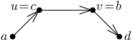
For every legal , we contract the paths as follows: We remove all outgoing edges of and , all incoming edges of and , and all edges incident to or . Then we identify and as well as and . If consists of a single path, then we remove all vertices except the two endpoints of this path, and we identify these two endpoints.
In this way, we obtain a slightly smaller instance . Then, for every , we remove the th objective to obtain , and recurse on with only objectives . This yields approximate Pareto curves of Hamiltonian cycles of . Now consider any . We expand the contracted paths to obtain . Then we construct two tours: First, we just add to , which yields a Hamiltonian cycle by construction. Second, we observe that no edge in is incident to or . We add the edge to as well as some more edges such that we obtain a Hamiltonian cycle. We put the Hamiltonian cycles thus constructed into .
We have not yet discussed the success probability. Randomness is needed for computing the approximate Pareto curves of cycle covers and the recursive calls of with objectives. Let be the size of the instance at hand, and let is a polynomial that bounds the size of a approximate Pareto curve from above. Then we need at most recursive calls of . In total, the number of calls of randomized algorithms is bounded by some polynomial . We amplify the success probabilities of these calls such that the probability is at least . Thus, the probability that one such call is not successful is at most by a union bound. Hence, the success probability of the algorithm is at least .
Instead of , we can also use its randomized counterpart . We modify such that the running-time is guaranteed to be polynomial and that there is only a small probability that errs. Furthermore, we have to make the error probabilities of the cycle cover computation as well as the recursive calls of slightly smaller to maintain an overall success probability of at least .
Overall, the running-time of is polynomial in the input size and , which can be seen by induction on : We have a polynomial time approximation algorithm for . For , the approximate Pareto curve of cycle covers can be computed in polynomial time, yielding a polynomial number of cycle covers. All further computations can also be implemented to run in polynomial time since for runs in polynomial time by induction hypothesis.
Theorem 4.1.
is a randomized approximation for multi-criteria Max-ATSP. Its running-time is polynomial in the input size and .
Proof.
We have already discussed the error probabilities and the running-time. Thus, it remains to consider the approximation ratio, and we can assume in the following, that all randomized computations are successful. We prove the theorem by induction on . For , this follows since mono-criterion Max-ATSP can be approximated with a factor .
Now assume that the theorem holds for . We have to prove that, for every Hamiltonian cycle , there exists a Hamiltonian cycle with . Since every Hamiltonian cycle is in particular a cycle cover, there exists a with . Now we distinguish two cases.
The first case is that consists solely of light-weight edges, i. e., , then returns a collection of paths with , which yields a Hamiltonian cycle with as claimed.
The second case is that contains at least one heavy-weight edge . Let , , , and be the edges in that are incident to or . (We may have some equalities among the vertices as shown in Figure 2.) Note that does not necessarily contain the edge . We consider the corresponding and divide the second case into two subcases.
The first subcase is that there exists a with , i. e., at least a fraction of the th objective is concentrated in . (We can have , but this is not necessarily the case.) Let be the set of such .
We fix one arbitrarily and consider the graph obtained by removing the th objective and contracting the paths and . A fraction of of the weight of is left in with respect to all objectives but those in . Thus, contains a Hamiltonian cycle with for all . Since -criteria Max-ATSP can be approximated with a factor of by assumption, contains a Hamiltonian cycle with for all . Together with , which contributes enough weight to the objectives in , we obtain a Hamiltonian cycle with , which is as claimed.
The second subcase is that for all . Thus, at least a fraction of of the weight of is outside of . We consider the case with the th objective removed. Then, with the same argument as in the first subcase, we obtain a Hamiltonian cycle of with for all . To obtain a Hamiltonian cycle of , we take the edge and connect its endpoints appropriately. (For instance, if are distinct, then we add the path and the edge .) This yields enough weight for the th objective in order to obtain a Hamiltonian cycle with since . ∎
4.2 Multi-Criteria Max-STSP
works of course also for undirected graphs, for which it achieves an approximation ratio of . But we can do better for undirected graphs.
Our algorithm for undirected graphs (Algorithm 4) starts by computing an approximate Pareto curve of cycle covers just as did. Then we consider each cycle cover separately. If consists solely of light-weight edges, then we can decompose using . If contains one or more heavy-weight edges, then some more work has to be done than in the case of directed graphs. The reason is that we cannot simply contract paths – this would make the new graph (and the edge weights ) asymmetric.
So assume that a cycle cover contains a heavy-weight edge . Let be such that . In a first attempt, we remove the th objective to obtain . Then we set for all edges incident to or . We recurse with objectives on with edge weights . This yields a tour on . Now we remove all edges incident to or of and add new edges including . In this way, we get enough weight with respect to objective . Unfortunately, there is a problem if there is an objective and an edge incident to or such that contains almost all weight with respect to : We cannot guarantee that this edge is included in without further modifying . To cope with this problem, we do the following: In addition to and , we set the weight of all edges incident to the other vertex of to . Then we recurse. Unfortunately, there may be another objective that now causes problems. To solve the whole problem, we iterate over all and over all additional vertices . Let . We remove one objective to obtain , set the weight of all edges incident to to , and recurse with objectives. Although the time needed to do this is exponential in , we maintain polynomial running-time for fixed .
As in the case of directed graphs, we can make the success probability of every randomized computation small enough to maintain a success probability of at least .
The base case is now : In this case, every cycle cover possesses a decomposition, and we do not have to care about heavy-weight edges. Overall, we obtain the following result.
Theorem 4.2.
is a randomized approximation for multi-criteria Max-STSP. Its running-time is polynomial in the input size and .
Proof.
We have already dealt with error probabilities and running-time. Thus, we can assume that all randomized computations are successful in the following. What remains to be analyzed is the approximation ratio. As in the proof of Theorem 4.1, the proof is by induction on .
The base case is . Let be an arbitrary Hamiltonian cycle. Then there is a with . From , we obtain a Hamiltonian cycle with by decomposition and Lemma 3.3.
Let us analyze for objectives. By the induction hypothesis, we can assume that is a approximation for -criteria Max-STSP. Let be any Hamiltonian cycle. We have to show that contains a Hamiltonian cycle with .
There is a with . We have to distinguish two cases. First, if consists solely of light-weight edges, i. e., for all , then we obtain a Hamiltonian cycle from with .
Second, let and with . We construct sets , , and in phases as follows (we do not actually construct these sets, but only need them for the analysis): Initially, and . In every phase, we consider the set of all edges of that have exactly one endpoint in . We always have by construction. Let . If is empty, then we are done. Otherwise, add to , add to , and add all new endpoints of vertices in to . We add at least one element to in every phase. Thus, and since .
Let , and let be the weight of edges of that have exactly one endpoint in . Let . By construction, we have for all . Otherwise, we would have added more edges to .
We distinguish two subcases. The first subcase is that . Then and . Consider the set and the edge weights used to obtain it. We have for . By the induction hypothesis, there is an with
for . We remove all edges incident to or to obtain . Since the weight of all these edges has been set to , we have . There exists a set such that and is a Hamiltonian cycle. For this cycle, which is in , we have
and, for ,
The second subcase is that is not empty. Let , and let . We consider . Let , , and be as defined above. By the induction hypothesis, the set contains a Hamiltonian cycle cover with for . We remove all edges incident to from to obtain with . By construction is a collection of paths. We add edges to to obtain such that is a Hamiltonian cycle. Let us estimate the weight of . For all , we have . For all , we have
which completes the proof. ∎
5 Remarks
The analysis of the approximation ratios of our algorithms is essentially optimal: Our approach can at best lead to approximation ratios of for some . The reason is as follows: Assume that -criteria Max-TSP can be approximated with a factor of . If we have a -criteria instance, we have to set the threshold for heavy-weight edges somewhere. Assume for the moment that this threshold be arbitrary. Then the ratio for -criteria Max-TSP is . Choosing maximizes this ratio. Thus, if for some , then . We conclude that the denominator of the approximation ratio increases by at least if we go from to .
For undirected graphs, we have obtained a ratio of roughly , which is optimal since implies . Similarly, for directed graphs, we have a ratio of , which is also optimal since implies .
Due to the existence of -decompositions, we conjecture that both -criteria Max-STSP and -criteria Max-ATSP can in fact be approximated with factors of . This, however, requires a different approach or at least a new technique for heavy-weight edges.
References
- [1] Ravindra K. Ahuja, Thomas L. Magnanti, and James B. Orlin. Network Flows: Theory, Algorithms, and Applications. Prentice-Hall, 1993.
- [2] Zhi-Zhong Chen, Yuusuke Okamoto, and Lusheng Wang. Improved deterministic approximation algorithms for Max TSP. Information Processing Letters, 95(2):333–342, 2005.
- [3] Matthias Ehrgott. Multicriteria Optimization. Springer, 2005.
- [4] Wassily Hoeffding. Probability inequalities for sums of bounded random variables. Journal of the American Statistical Association, 58(301):13–30, 1963.
- [5] Haim Kaplan, Moshe Lewenstein, Nira Shafrir, and Maxim I. Sviridenko. Approximation algorithms for asymmetric TSP by decomposing directed regular multigraphs. Journal of the ACM, 52(4):602–626, 2005.
- [6] Bodo Manthey. Approximate pareto curves for the asymmetric traveling salesman problem. Computing Research Repository cs.DS/0711.2157, arXiv, 2007.
- [7] Bodo Manthey. On approximating restricted cycle covers. SIAM Journal on Computing, 38(1):181–206, 2008.
- [8] Bodo Manthey and L. Shankar Ram. Approximation algorithms for multi-criteria traveling salesman problems. Algorithmica, to appear.
- [9] Ketan Mulmuley, Umesh V. Vazirani, and Vijay V. Vazirani. Matching is as easy as matrix inversion. Combinatorica, 7(1):105–113, 1987.
- [10] Christos H. Papadimitriou and Mihalis Yannakakis. On the approximability of trade-offs and optimal access of web sources. In Proc. of the 41st Ann. IEEE Symp. on Foundations of Computer Science (FOCS), pages 86–92. IEEE Computer Society, 2000.