Opportunistic Interference Alignment in MIMO Interference Channels
Abstract
We present two interference alignment techniques such that an opportunistic point-to-point multiple input multiple output (MIMO) link can reuse, without generating any additional interference, the same frequency band of a similar pre-existing primary link. In this scenario, we exploit the fact that under power constraints, although each radio maximizes independently its rate by water-filling on their channel transfer matrix singular values, frequently, not all of them are used. Therefore, by aligning the interference of the opportunistic radio it is possible to transmit at a significant rate while insuring zero-interference on the pre-existing link. We propose a linear pre-coder for a perfect interference alignment and a power allocation scheme which maximizes the individual data rate of the secondary link. Our numerical results show that significant data rates are achieved even for a reduced number of antennas.
I Introduction
We consider the case of radio devices attempting to opportunistically exploit the same frequency band being utilized by licensed networks under the constraint that no additional interference must be generated. This can be implemented for example by assuming that opportunistic users are cognitive radios [1, 2]. Typically, cognitive radios temporally exploit the unused frequency bands, named white-spaces, to transmit their data. This clearly improves the spectral efficiency since more users are allowed to co-exist in the same bandwidth. However, a higher spectrum efficiency could be attained by simultaneously allowing the opportunistic radios to transmit with the licensees if no harmful interference is generated. In this case, interference alignment (IA) has been identified as a powerful tool to achieve such a goal. This technique, was initially introduced in [3, 4]. IA allows a given transmitter to partially or completely “align” its interference with unused dimensions of the primary terminals [5]. The concept of dimension could be associated with a specific spatial direction, frequency carrier or time slot [4], [6]. An extensive study has been conducted [4, 6, 7] to estimate the number of interference-free dimensions a given radio might find to transmit when several radio systems co-exist. In [4] and [6] several IA schemes to exploit such dimensions are proposed. Similarly, in [8], a linear pre-coder based on Vandermonde matrices allows an orthogonal frequency division multiplexing (OFDM) radio to co-exist with similar pre-existing terminals without generating any additional interference. The idea is to exploit the redundancy of the OFDM cyclic prefix and frequency selectivity of the channel.
In this study, we propose a novel interference alignment technique for the secondary users exploiting the fact that under a power-limitation, a primary user which maximizes its own rate by water-filling on its MIMO channel singular values, might leave some of them unused. i.e. no transmission takes place along the corresponding spatial directions. These unused directions may be opportunistically utilized by a secondary transmitter, since its signal would not interfere with the signal sent by the primary transmitter. We present a linear pre-coder which perfectly aligns the interference generated by the secondary transmitter with such unused spatial directions. Similarly, we present a power allocation scheme based on the water-filling idea which maximizes the individual data rate of the opportunistic radio. Simulation results show that a significant data rate can be achieved by the secondary link following our approach.
II System Model
Notation: In the following, matrices and vectors are denoted by boldface upper case symbols and boldface lower case symbols, respectively. The entry of the vector is denoted . The entry corresponding to the row and column of the matrix is denoted by . The -dimension identity and null matrix are represented by and , respectively. The Hermitian transpose is denoted , and the expected value is represented by the operator .
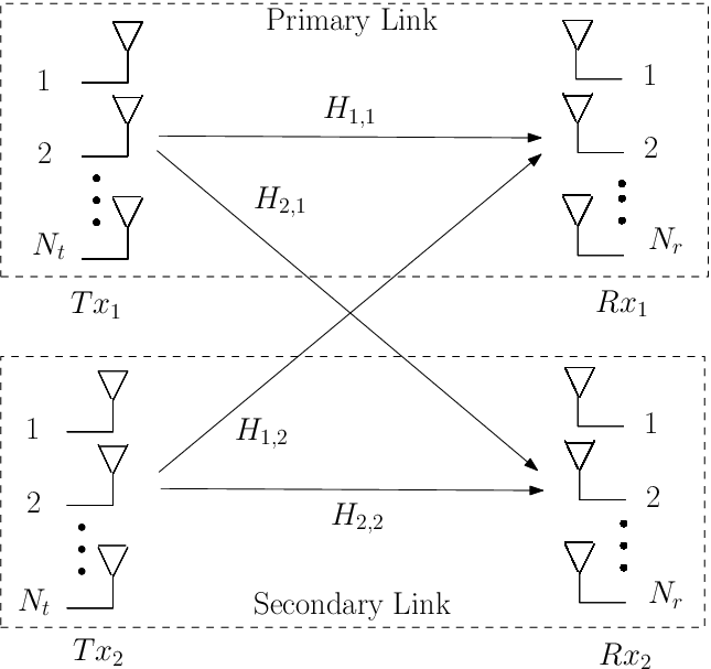
We consider two point-to-point unidirectional links simultaneously operating in the same frequency band and producing mutual interference as shown in Fig. 1 [9]. Both transmitters are equipped with antennas while both receivers use antennas. The first transmitter-receiver pair, i.e. and , is a primary link licensed to exclusively exploit a given frequency band. The pair, and is an opportunistic link exploiting the same frequency band subject to the constraint that no additional interference must be generated over the primary system. Note that no cooperation between terminals is allowed, i.e. transmitters do not share or exchange any signal before transmitting. Therefore, the multiple access interference (MAI) is considered as additive white Gaussian noise (AWGN).
The channel transfer matrix from transmitter to receiver is denoted , where the entries of are independent and identically distributed (i.i.d) complex Gaussian circularly symmetric random variables. The channel matrices are supposed to be fixed for the whole transmission duration. This correspond to assuming (static) Gaussian links. But our analysis readily extends to the case of slow-fading channels by assuming the channels to be constant over each data block. Regarding the channel state information (CSI) conditions, we assume the primary terminals (transmitter and receiver) to only have perfect knowledge of the matrix . On the other hand, the secondary terminals have perfect knowledge of all the channel transfer matrices , for every and . Although unrealistic, this condition provides us with an upper bound on the achievable rate of the secondary user. It can however be met in practice in the TDD (Time Division Duplex) mode if the secondary user exploits opportunistically the training sequences and signaling communication between the primary devices.
Following a matrix notation, the primary and secondary received signals can be written as
| (1) |
where the vectors and represent the transmitted symbols and an AWGN process with zero mean and covariance matrix for the link. For all the matrices represent the linear pre-coders used for interference alignment. Furthermore, at each receiver, the input signal is linearly processed with the matrix . The signal at the output of the linear filter is . Both matrices and are described later on. The power allocation matrices are defined as the input covariance matrices , for the transmitter. The power constraints are
| (2) |
where is the maximum transmit power level for the transmitter. Without loss of generality, we assume identical maximum transmit powers for all the terminals i.e. , .
III Interference Alignment Strategy
In this section we focus on the study of the pre-coding and post-processing matrices. Suppose that the primary terminals completely ignore the presence of the opportunistic transmitter. Hence, in order to maximize its own data rate, the primary transmitter follows a water-filling power allocation as in the single-user case [10].
III-A Primary link design
Under the assumption that the channel matrix is known at the receiver and transmitter, the primary terminal chooses its pre-coding and post-processing matrices in such a way that their channel transfer matrix is diagonalized, i.e. and satisfy the singular value decomposition , where and are unitary matrices and is a diagonal matrix which contains non-zero singular values, . Thus, the received signal after linear processing, , can be written as
| (3) |
where is an AWGN process with zero mean and covariance matrix . Then, the achievable rate of the primary user is maximized by the power allocation matrix which is a solution to the following optimization problem
| (4) |
The solution to (4) is the classical water-filling algorithm [10]. Following this approach, the optimal power allocation matrix is a diagonal matrix with entries
| (5) |
with . The constant is a Lagrangian multiplier that is determined to satisfy
III-B Secondary link design
Depending on the channel singular values , the power allocation matrix might contain zeros in its main diagonal. A zero power allocation for a given singular value means that no transmission takes place along the corresponding spatial direction. This means that the secondary terminal can align its transmitted signal with the unused singular modes such that it does not interfere with the signal transmitted by the primary user. If one converts the spatial problem into the frequency one, the result is similar to the cognitive scenario where the secondary would opportunistically use the unexploited frequency modes. The main difference here lies in the fact that in the spatial domain, there is no universal precoder which diagonalizes the basis of all the devices whereas this is the case in the frequency domain with the use of the FFT.
As a consequence, in the spatial domain, the corresponding orthogonality condition (such that the secondary user generates no interference on the primary link) is given by
| (6) |
where the matrix is a diagonal matrix with entries
| (7) |
such that the condition always holds. It can be easily verified since both matrices are diagonal. Additionally, the constant is chosen to satisfy the power constraints (2) with .
Assuming that perfect estimates of and are available at the secondary transmitter, the secondary precoder (when the inverse of exists) is given by:
| (8) |
For the case where , i.e. the receiver has more antennas than the transmitter, it is still possible to obtain the pre-coding matrix by using the Moore-Penrose pseudo-inverse of ,
| (9) |
Once the pre-decoder has been adapted to satisfy (8) or (9) at the secondary transmitter, no additional interference impairs the primary user. However, the secondary receiver still undergoes the interference from the primary transmitter. Typically, this effect is a colored noise with covariance due to the channel and the pre-coder . Here,
| (10) |
Hence, the received signal can be whitened by using the matrix , to obtain , such that
| (11) |
where is an i.i.d. AWGN process with zero mean and a covariance matrix proportional to the identity. Let be the number of zeros on the main diagonal of . Then, the matrix contains zero columns. Note that implies that no transmission takes place in the secondary link. In the sequel, we always assume that (which will be the case at low signal to noise ratio as shown in the simulations).
IV Input Covariance Matrix Optimization
In the latter section the proposed pre-coding scheme does not generate any interference on the primary user but the transmission rate for the secondary user was not optimized. For this purpose, the choice of the power allocation of the secondary transmitter, i.e. the matrix , needs to be optimized. First, we present the most simple case where uniform power allocation is performed. Second, we introduce a power allocation which maximizes the individual transmission rate. In both cases we assume that the pre-coder has been previously adapted to satisfy the orthogonality conditions (8) or (9).
IV-A Uniform Power Allocation
For the uniform power allocation scheme the input covariance matrix is set to and the constant from (6) is tuned in order to meet the condition . The rate achieved by the secondary user while generating zero-interference to the primary receiver is
| (12) |
IV-B Optimal Power Allocation
The transmission rate for the secondary link is maximized by adopting a power allocation matrix which is a solution of the following optimization problem,
| (13) |
where
| (14) |
Note that solving this optimization problem requires the knowledge of the covariance matrix , which is calculated at the secondary receiver based on the knowledge of the channel . This can be done if the secondary receiver estimates and feeds it back to the secondary transmitter. Here, we assume a perfect knowledge of is available at the secondary transmitter.
By definition (Eq. (13)), the matrix is not full rank. Therefore, the optimization problem (13) does not have a simple solution. We propose a two-step optimization which leads to a water-filling solution. First, we define a new input covariance such that,
| (15) |
By replacing the expression (15) in (13), the optimization problem becomes
| (16) |
where . The idea here is to solve the a priori non-trivial optimization problem defined by expression (13) by introducing an equivalent channel matrix to simplify the problem. Using we can then apply a singular value decomposition to the new channel such that , where and are unitary matrices, and the matrix contains the singular values of . Under these assumptions, the optimal solution is
| (17) |
where is a Lagrangian multiplier that is determined to satisfy . Once has been obtained, then the optimal power allocation matrix [10] is
| (18) |
The constant in (6) is tuned such that the condition (2) is met for .
V Numerical Results
In this section we show numerical examples to illustrate the performance of our interference alignment strategy. Considering the same number of antennas at the receiver and the transmitter, we analyze the number of unused singular values or free dimensions available for the secondary link as well as its achieved data rate. Recall that the primary link is interference-free, therefore its data rate corresponds to the single user case rate [10].
In Fig. 2 we show the number of unused singular values in the primary link as a function of the number of antennas and . Note that in low SNR regime, the transmitter attempts to concentrate all its power in the best singular values leaving all the others unused. On the contrary, in high SNR regime the primary transmitter tends to spread its power among all its available singular values. Thus, in the first case the opportunistic link has plenty of free dimensions, while in the second one, it is effectively limited. This power allocation behavior has been also reported in [11] and [12]. Similarly, it is observed that increasing the number of antennas leads on average, to a linear scaling of the unused singular values. In Fig. 3, we show the achieved data rate of secondary link when optimal power allocation is implemented () as a function of the number of antennas and the SNR. Therein, it is shown that at very low and very high SNRs the data rate approaches zero bits/sec. In low SNR regime this effect is natural since detection is difficult due to the noise. However, at high SNRs it is due to the fact that the primary transmitter does not leave any unused singular value. Nonetheless, at intermediate SNRs, significant data rates are achieved by the secondary link. Note that increasing the number of antennas always leads to higher data rates for the secondary link. In Fig. 4, we plot the data rate of the primary and secondary link for the case of uniform and optimal power allocation. Note that in high SNR regime, the and performs similarly. It is due to the fact that few or even none of the singular values are left unused by the primary link, therefore the uniform power allocation does not differ from the optimal in average. In contrast, at intermediate SNRs the difference in performance is more significant for a large number of antennas.


VI Conclusions
We provided a novel interference alignment scheme which allows an opportunistic point-to-point MIMO link to co-exist with a similar pre-existing primary link on the same fully utilized band without generating any additional interference. The proposed scheme exploits the fact that the licensed transmitter, while performing water-filling power allocation on its MIMO channel (in order to maximize its single user rate) will leave some singular values unused when constrained by power limitations. Hence, no transmission takes place along the corresponding spatial directions. We proposed a linear pre-coder for the opportunistic radio, which perfectly aligns the transmitted signal with such unused dimensions. We also provided a power allocation scheme which maximizes the data rate of the opportunistic link. Numerical results show that significant data rates are achieved by the secondary link even for a reduced number of antennas. Further studies will extend the novel approach to multi-user multi-carrier systems and the case of incomplete CSI.
References
- [1] S. Haykin, “Cognitive radio: brain-empowered wireless communications,” Selected Areas in Communications, IEEE Journal on, vol. 23, no. 2, pp. 201–220, 2005.
- [2] B. A. Fette, Cognitive Radio Technology. Newnes editors, 2006.
- [3] M. Maddah-Ali, A. Motahari, and A. Khandani, “Communication over x channel: Signalling and multiplexing gain,” UW-ECE-2006-12, University of Waterloo, Tech. Rep., July 2006.
- [4] M. A. Maddah-Ali, A. S. Motahari, and A. K. Khandani, “Signaling over mimo multi-base systems: Combination of multi-access and broadcast schemes,” in Information Theory, 2006 IEEE International Symposium on, 2006, pp. 2104–2108.
- [5] V. R. Cadambe and S. A. Jafar, “Interference alignment and spatial degrees of freedom for the k user interference channel,” in Communications, 2008. ICC ’08. IEEE International Conference on, 2008, pp. 971–975.
- [6] S. A. Jafar and M. J. Fakhereddin, “Degrees of freedom for the mimo interference channel,” Information Theory, IEEE Transactions on, vol. 53, no. 7, pp. 2637–2642, 2007.
- [7] S. A. Jafar and S. Shamai, “Degrees of freedom region of the mimo x channel,” Information Theory, IEEE Transactions on, vol. 54, no. 1, pp. 151–170, 2008.
- [8] L. S. Cardoso, M. Kobayashi, M. Debbah, and O. Ryan, “Vandermonde frequency division multiplexing for cognitive radio,” in SPAWC2008, July 2008.
- [9] H. Sato, “Two-user communication channels,” Information Theory, IEEE Transactions on, vol. 23, no. 3, pp. 295–304, 1977.
- [10] W. Yu, W. Rhee, S. Boyd, and J. M. Cioffi, “Iterative water-filling for gaussian vector multiple-access channels,” Information Theory, IEEE Transactions on, vol. 50, no. 1, pp. 145–152, 2004.
- [11] F. R. Farrokhi, A. Lozano, G. J. Foschini, and R. A. Valenzuela, “Spectral efficiency of fdma/tdma wireless systems with transmit and receive antenna arrays,” Wireless Communications, IEEE Transactions on, vol. 1, no. 4, pp. 591–599, 2002.
- [12] C.-N. Chuah, D. N. C. Tse, J. M. Kahn, and R. A. Valenzuela, “Capacity scaling in mimo wireless systems under correlated fading,” Information Theory, IEEE Transactions on, vol. 48, no. 3, pp. 637–650, 2002.