Optimal View Angle in Collective Dynamics of Self-propelled Agents

The collective motion of a group of autonomous agents (or particles) [1, 2, 3, 4, 5, 6, 7, 8] has attracted much attention in the past decade. One of the most remarkable characteristics of systems, such as flocks of birds, schools of fish, and swarms of locusts, is the emergence of collective states in which the agents move in the same direction. A particularly simple and popular model to describe such behavior was proposed by Vicsek et al. [9]. Due to simplicity and efficiency, the Vicsek model (VM) has been intensively investigated in recent years [10, 11, 12, 13, 14, 15, 16, 17, 18, 19, 20, 21, 22].

In the VM, $N$ agents move synchronously in a square shaped cell of linear size $L$ with the periodic boundary conditions. The initial directions and positions of the agents are randomly distributed in the cell, and each agent has the same absolute velocity $v_{0}$. Agent $i$ and agent $j$ are neighbors at time step $k$ if and only if $\parallel\vec{X}_{i}(k)-\vec{X}_{j}(k)\parallel\leq R$, where $\vec{X}_{i}(k)$ denotes the position of agent $i$ on a 2-dimensional (2D) plane at time step $k$ and $R$ is the sensor radius. The direction of agent $i$ at time step $k+1$ is:

where $\langle\theta_{i}(k)\rangle_{R}$ denotes the average direction of agent $i$’s neighbors (include itself), $\Delta\theta$ denotes noise (in the following discussions, $\Delta\theta=0$ without special mention). To be more specific, let $\Gamma_{i}(k)$ be the set of neighbors of agent $i$ at time step $k$, the VM is then described as [16, 17]:

where $e^{i\theta_{i}(k)}$ is the unitary complex directional vector of agent $i$, $e^{i\theta_{i}(k)}=\cos(\theta_{i}(k))+i\sin(\theta_{i}(k))$, $\theta_{i}(k)\in[0,2\pi)$. Here the function $angle(\cdot)$ denotes the angle of a complex number. $\theta_{i}(k+1)$ is the moving direction of agent at time step $k+1$, which is the average direction of agents in the neighbor set $\Gamma_{i}(k+1)$. $v_{0}e^{i\theta_{i}(k)}$ represents the velocity of agent $i$ at time step $k$ with constant speed $v_{0}$ and direction $\theta_{i}(k)$.

In the VM and most other models of self-propelled particles, the field of vision for every agent is a complete disc (2D case) or a sphere (3D case) characterized only by its sensor radius $R$. In the reality, however, most animals are incapable of complete view. For example, the cyclopean retinal field of human is about 180 degree and the cyclopean retinal field of tawny owl is 201 degree [23]. It is thus more reasonable to assume limited view angles of agents [3, 24], instead of the omnidirectional views, in swarm models to better mimic the real collective behaviors.

In this Brief Report, we investigate the VM in which agents have limited view angles $\omega$, $\omega\in(0,2\pi]$. As illustrated in Fig. 1, the field of vision of every agent is only a sector of disc bounded by two radii and the included arc, the left (right) boundary of vision and the heading of agent $i$ have inclination $\omega/2$, that is, for every agent, the field of view is symmetric about its current moving direction. Thus rule (3) in the VM can be modified as:

where $\Gamma_{i}(k+1,\omega)$ denotes the neighbor set of agent $i$ with view angle $\omega$. When $\omega=2\pi$, the rule (4) degenerates to the original Vicsek model (3).

To give a quantitative discussion, we define an order parameter

for the system (4) at time step $k$ with view angle $\omega$, obviously, $0\leq\Phi(k,\omega)\leq 1$.

In noiseless case, the order parameter $\Phi(k,\omega)$ can approach 1 when the evolution is long enough, except for extremely rare cases (for example, the cases may occur when $R$ or $\omega$ is too small). To quantify the speed of direction consensus, we study the transient time step $\tau$, which is defined as the time step when the order parameter first surpasses a certain value $\Phi_{0}$. Here we take $\Phi_{0}=0.99$ and we have checked that qualitative results are not changed when $\Phi_{0}$ is large enough.

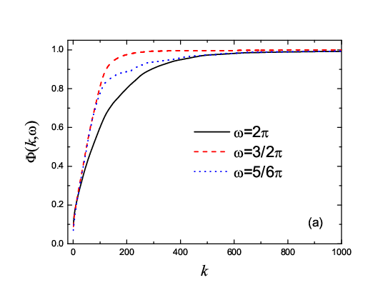
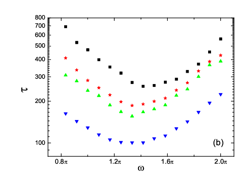
We then investigate the effects of the view angle $\omega$ on the transient process. As shown in Fig. 2(a), the order parameter $\Phi(k,\omega)$ reaches 1 faster when the view angle $\omega=3\pi/2$, compared with $\omega=2\pi$ and $\omega=5\pi/6$. Figure 2(b) shows the transient time step $\tau$ as a function of $\omega$ for different values of parameters. One can find that $\tau$ is not a monotonic function of $\omega$ and there exists an optimal view angle, leading to the shortest transient time.

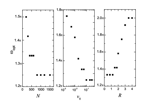
Figure 3 shows the optimal view angle $\omega_{opt}$ as functions of the parameters: the swarm number $N$, the sensor radius $R$ and the absolute velocity $v_{0}$, respectively. One can see that the optimal view angle $\omega_{opt}$ decreases with the increasing of $N$ and $v_{0}$, and converges to a fixed value when $N$ or $v_{0}$ is large enough. $\omega_{opt}$ increases as the sensor radius $R$ increases. In particular, when $R$ being close to the lattice size $L$, agents with panoramic view will be globally coupled and the directions of the swarm can reach consensus in only one time step.

We next investigate whether more communications are needed for faster convergence. We define $n_{i}(k,\omega)$ as the number of $i$’s neighbors, and the average number of neighbors $\langle n(k,\omega)\rangle$ over all agents at time step $k$ is

In Fig. 4, we report this average neighboring number for different $\omega$. Combining Fig. 2(a) and Fig. 4, it is interesting to find that, agents with optimal view angle $\omega=3\pi/2$ have the least number of neighbors in the steady state, compared with $\omega=2\pi$, $\omega=5\pi/6$ and $\omega=\pi$. This result indicates the existence of superfluous communications in the VM, which may counteract the direction consensus.

In the following, we focus on the noise effects associated with the restriction of view angle. The noise is introduced to the view angle model as:

where the moving direction of each agent is perturbed by a random number $\xi$ chosen with a uniform probability from the interval $[-\eta,\eta]$. In the presence of noise, the order parameter $\Phi(k,\omega,\eta)$ will fluctuate and never keep fixed at a certain value, therefor we adopt a statistically stable order parameter in terms of $\Phi_{stable}(\omega,\eta)$, which is an average of the consecutive series of $\Phi(k,\omega,\eta)$ over many time steps after a sufficiently long transient time. Figure 5 shows that $\Phi_{stable}(\omega,\eta)$ increases as $\omega$ increases if the noise is kept constant, and decreases as the noise increases.

In the noisy case, we define the transient time step $\tau$ as the time step when the order parameter firstly exceeds $0.99\Phi_{stable}(\omega,\eta)$ for each run. For $\eta=0$, $\Phi_{stable}(\omega,0)$ approaches 1, thus this definition of $\tau$ is applicable in the absence of noise. From Fig. 6, one can find that there still exists an optimal view angle $\omega_{opt}$ leading to the shortest transient time step in the presence of noise and the value of the optimal view angle decreases as the noise increases.

In conclusion, we have studied the effects of restricted vision of a group of self-propelled agents. The field of vision of every agent is only a sector of disc and the included arc represents the view angle. It is interesting to find that there exists an optimal angle resulting in the fastest direction consensus. The value of the optimal view angle increases as the increasing of sensor radius, while decreases as the increasing of swarm number, the absolute velocity or the noise strength. Another interesting phenomenon is that agents with optimal view angle have the least number of neighbors in the steady state. Our studies indicate the existence of superfluous communications in the Vicsek model, which indeed hinder the direction consensus. Moreover, our results may be useful in designing the man-made swarms such as autonomous mobile robots.

We thank Hai-Tao Zhang and Ming Zhao for their valuable comments. This work is funded by the National Basic Research Program of China (973 Program No.2006CB705500), the National Natural Science Foundation of China under Grant Nos. 10635040 and 10805045, the Specialized Research Fund for the Doctoral Program of Higher Education of China (20060358065).

References

- [1] J. K. Parrish, Science 284, 99 (1999).
- [2] H. Levine, W. J. Rappel, and I. Cohen, Phys. Rev. E 63, 017101 (2000).
- [3] I. D. Couzin, J. Krause, R. James, G. D. Ruxton, and N. R. Franks, J. Theor. Biol. 218, 1 (2002).
- [4] I. D. Couzin, J. Krause, N. R. Franks, and S. A. Levin, Nature (London) 433, 513 (2005).
- [5] J. Buhl, D. J. T. Sumpter, I. D. Couzin, J. J. Hale, E. Despland, E. R. Miller, and S. J. Simpson, Science 312, 1402 (2006).
- [6] M. R. D’Orsogna, Y. L. Chuang, A. L. Bertozzi, and L. S. Chayes, Phys. Rev. Lett. 96, 104302 (2006).
- [7] D. Grunbaum, Science 312, 1320 (2006).
- [8] A. Kolpas, J. Moehlis, and I. G. Kevrekidis, Proc. Natl. Acad. Sci. U.S.A. 104, 5931 (2007).
- [9] T. Vicsek, A. Czirók, E. Ben-Jacob, I. Cohen, and O. Shochet, Phys. Rev. Lett. 75, 1226 (1995).
- [10] L. Moreau, IEEE Trans. Autom. Control 50, 169 (2005).
- [11] F. Cucker and S. Smale, IEEE Trans. Autom. Control 52, 852 (2007).
- [12] G. Grégoire and H. Chaté, Phys. Rev. Lett. 92, 025702 (2004).
- [13] C. Huepe and M. Aldana, Phys. Rev. Lett. 92, 168701 (2004).
- [14] M. Aldana, V. Dossetti, C. Huepe, V. M. Kenkre, and H. Larralde, Phys. Rev. Lett. 98, 095702 (2007).
- [15] M. Nagy, I. Daruka, and T. Vicsek, Physica A 373, 445 (2007).
- [16] W. Li and X. F. Wang, Phys. Rev. E 75, 021917 (2007).
- [17] W. Li, H. T. Zhang, M. Z. Q. Chen, and T. Zhou, Phys. Rev. E 77, 021920 (2008).
- [18] W. Li, IEEE Trans. Syst., Man, Cybern. B 38, 1084 (2008).
- [19] H. Chaté, F. Ginelli, G. Grégoire, and F. Raynaud, Phys. Rev. E 77, 046113 (2008).
- [20] H. T. Zhang, M. Chen, and T. Zhou, Phys. Rev. E 79, 016113 (2009).
- [21] L. Q. Peng, Y. Zhao, B. M. Tian, J. Zhang, B. H. Wang, H. T. Zhang, and T. Zhou, Phys. Rev. E 79, 026113 (2009).
- [22] J. Zhang, Y. Zhao, B. M. Tian, L. Q. Peng, H. T. Zhang, B. H. Wang, and T. Zhou, Physica A 388, 1237 (2009).
- [23] G. R. Martin, J Comp Physiol A 174, 787 (1994)
- [24] A. Hutha and C. Wissela, J. Theor. Biol. 156, 3 (1992).