Failure of Local Realism Revealed by Extremely Coarse-Grained Measurements

The development of quantum physics has revealed a world quite different from the one depicted by classical physics. Probably, the most striking feature of the quantum world, distinguishing it from the classical one, is failure of local realism [1, 2]. Local realism combines two reasonably acceptable assumptions, locality and realism. The principle of locality is that distant objects cannot have direct instantaneous influence on one another. Physical realism claims that all measurement outcomes are determined by pre-existing quantities of physical systems. The failure of local realism is evidenced by violation of Bell’s famous inequality which should be obeyed by any local-realistic theories.

Although certain odd features of nature predicted by quantum physics such as the failure of local realism have been experimentally observed in laboratories [3, 4], such quantum properties are not seen in our everyday experience on a macroscopic scale. Decoherence is often considered the main reason for the appearance of the classical world from the laws of quantum physics [5]. Quantum systems, particularly when they are macroscopic, unavoidably interact with their environments and rapidly lose their quantum features. Recently, Kofler and Brukner suggested a conceptually different view [6]: they attributed the appearance of the classical world to the “coarse-grained” (or fuzzy) properties of the measurements, suggesting that “classical physics can be seen as implied by quantum mechanics under the restriction of fuzzy measurements.”

Here, we address a crucial question concerning fundamental tests of quantum mechanics: Can the quantum world where local realism fails be perceived by the observer even when the measurements are very unsharp? In stark contrast with the conclusions reached in [6], here we find that extremely coarse-grained measurements can still be useful to reveal the quantum world where local realism fails. In our examples, Bell’s inequality, which is enforced by local realism, is violated up to the maximum limit, known as Cirel’son’s bound [7], when appropriate local unitary transformations and states are chosen alongside the coarse-grained measurements. Furthermore, we show that while local realism fails, a recent version of Leggett’s inequality [8, 9, 10], which is imposed by non-local realistic theories, can still be satisfied. Failure of local realism means that at least one between locality and realism should be abandoned while the satisfaction of Leggett’s inequality implies that a realistic interpretation is tenable as far as some level of non-locality is allowed. This suggests that locality alone fails while realism is tenable in our specific examples.

In order to show such instances, we first need to describe the sort of coarse-grained measurements we consider, which should only be able to discern differences at a macroscopic scale [6]. As an extreme example, a “measurement” by human eyes can notice differences between two objects only when they are macroscopically different. In quantum optics, homodyne measurements with low efficiency can be considered such coarse-grained measurements in the classical limit: two different states may be distinguished only when they are sufficiently separate in phase space. In our study, we make use of entangled thermal states (ETSs), which have been introduced in [11], where component states are “classical” thermal states. Of course, even when local states obtained by taking the partial trace of the total state appear classical, Bell’s inequality can be violated if “sharp” measurements, such as highly efficient photon number detection, are used as shown in [11, 12]. However, it has not been previously found that extremely unsharp measurements can be used to reveal failure of local realism.

In our proposal, two local parties, Alice and Bob, are each provided with one mode of an ETS prepared by a third party upon entangling two displaced thermal states as described in [11]. A displaced thermal state is defined as $\rho^{\rm th}(V,d)=\int d^{2}\alpha P_{\alpha}^{\rm th}(V,d)|\alpha\rangle\langle\alpha|$, where $P_{\alpha}^{\rm th}(V,d)=\frac{2}{\pi(V-1)}e^{-\frac{2|\alpha-d|^{2}}{V-1}}$ a Gaussian function with variance $V$ and center $d$ (with respect to the origin of the phase space). Two identical such states, $\rho^{\rm th}_{A}(V,d)$ and $\rho^{\rm th}_{B}(V,d)$, are distributed to spatially separate locations. As the first step to entangle them, a microscopic system in the superposition state, $|\psi\rangle_{m}=(|0\rangle_{m}+|1\rangle_{m})/\sqrt{2}$, sequentially interacts with the two thermal states, where, $|0\rangle_{m}$ and $|1\rangle_{m}$ are the ground and excited states of the microscopic system (for instance, the first two levels of a harmonic oscillator or two energy levels of an atom). The interaction is taken to be of the nonlinear cross-Kerr form ${\cal H}^{K}_{mj}=\hbar\lambda\hat{a}_{m}^{\dagger}\hat{a}_{m}\hat{a}_{j}^{\dagger}\hat{a}_{j}$ with $\lambda$ the strength of the nonlinearity and $j=A,B$. Nonlinear media with free-traveling optical fields [14, 15] or dispersive interactions within optical/microwave cavities [16] may be used to implement such interactions [11, 13]. We stress that the use of the microscopic superposition, $|\psi\rangle_{m}$, is not essential, and we shall later describe an alternative method using another type of ETS produced without it.

For simplicity, we assume that the interaction time is $t=\pi/\lambda$, while we note that an equivalent effect can be obtained in principle using a (more realistic) weaker nonlinearity ($t\ll\pi/\lambda$) and a thermal state with a larger displacement $d$ [15, 11]. When the thermal state $\rho^{\rm th}_{j}(V,d)$ interacts with the ground state $|0\rangle_{m}$, nothing happens. On the other hand, when it interacts with the excited state of $m$, it evolves to $\rho^{\rm th}_{j}(V,-d)$, i.e. it is “moved” to the opposite location in the phase space. After the interactions represented by ${\cal H}^{K}_{mA}\otimes{\cal H}^{K}_{mB}$, the microscopic system is measured out on the superposed basis $(|0\rangle\pm|1\rangle)_{m}/\sqrt{2}$. As the result, the thermal states at modes $A$ and $B$ become entangled [11, 13]. From now on, we assume that the outcome of the measurement is $(|0\rangle+|1\rangle)_{m}/\sqrt{2}$ so that the ETS $\rho_{AB}^{\Psi(+)}$ is shared between Alice and Bob who, as described below, should now perform nonlinear local operations and homodyne measurements.

The local operations required for Bell inequality tests are composed of displacement operation $\hat{D}_{j}(\zeta)=e^{\zeta\hat{a}^{\dagger}_{j}-\zeta^{*}\hat{a}_{j}}$ ($\zeta\in\mathbb{C}$) and single-mode Kerr nonlinearities described by the interaction Hamiltonian ${\cal H}_{NL,j}=\hbar\Omega({\hat{a}}^{\dagger}_{j}{\hat{a}}_{j})^{2}$, where $\Omega$ is the strength of the nonlinearity and $\hat{a}_{j}$ ($\hat{a}^{\dagger}_{j}$) is the annihilation (creation) operator of system $j$. The displacement operation $\hat{D}_{j}(\zeta)$ can be readily performed using a beam splitter and a thermal state with a large displacement. Nonlinear media such as optical crystals can in principle be used to realize single-mode Kerr effects. It is known that the Kerr nonlinear interaction, $\hat{U}_{NL}=e^{-\frac{i}{\hbar}{\cal H}_{NL}t_{c}}$, where $t_{c}=\pi/\Omega$, causes a coherent state to evolve into the normalized state $\hat{U}_{NL}|\alpha\rangle=e^{-i\frac{\pi}{4}}(|\alpha\rangle+i|-\alpha\rangle)/\sqrt{2}$ [17]. We define the local unitary operations [18] $\hat{\cal V}_{j}(\theta_{j})=\hat{U}_{NL,j}\hat{D}_{j}\left({i\theta_{j}}/{2d}\right)\hat{U}_{NL,j}$, which are applied to mode $j=A,B$ as ${\rho_{AB}^{\Psi{(+)}}}^{\prime}(\theta_{A},\theta_{B})=\hat{\cal V}_{A}(\theta_{A})\hat{\cal V}_{B}(\theta_{B}){\rho_{AB}^{\Psi{(+)}}}\hat{\cal V}^{\dagger}_{A}(\theta_{A})\hat{\cal V}^{\dagger}_{B}(\theta_{B})$.

An imperfect homodyne detector with efficiency $\eta$ can be modeled by a beam splitter with transmittivity $\eta$, superimposing mode $j$ ($j=A,B$) with an ancilla $v_{j}$ prepared in vacuum state, and cascaded with an ideal homodyne detector. The beam splitter operator between modes $j$ and $v_{j}$ is defined as ${\hat{B}}_{jv_{j}}=e^{\frac{\xi}{2}({\hat{a}}_{j}^{\dagger}{\hat{a}}_{v_{j}}-{\hat{a}}_{j}{\hat{a}}_{v_{j}}^{\dagger})}$, where $\cos\xi=\sqrt{\eta}$. As we discard the output state of the ancillae, this changes ${\rho_{AB}^{\Psi{(+)}}}^{\prime}(\theta_{A},\theta_{B})$ into ${\rho_{AB}^{\Psi{(+)}}}^{\prime}(\theta_{A},\theta_{B},\eta)={\rm Tr}_{v_{A,B}}\big[{\hat{B}}_{Av_{A}}{\hat{B}}_{Bv_{B}}{\rho_{AB}^{\Psi{(+)}}}^{\prime}(\theta_{A},\theta_{B})\big(|00\rangle_{v_{A}v_{B}}\!\langle{00}|\big){\hat{B}}^{\dagger}_{Av_{A}}{\hat{B}}^{\dagger}_{Bv_{B}}\big]$.

The tools described above bear some analogies with the qubit case: states $\rho^{\rm th}(V,\pm d)$ correspond to a qubit basis, the ETS a two-qubit entangled state, the nonlinear operation ${\cal V}_{j}(\theta_{j})$ a single-qubit operation, and the homodyne detection to discriminate between the two thermal states a computational basis measurement. In order to test Clauser, Horne, Shimony, and Holt (CHSH)’s version of Bell’s inequality [19], we assign value $+1$ to the measurement outcome corresponding to a homodyne signal larger than 0, and $-1$ otherwise. Then, the joint probability $P_{kl}(\theta_{A},\theta_{B})$, where the subscripts $k,l=\pm$ correspond to A and B’s assigned measurements outcomes $\pm{1}$ respectively, can be calculated as $P_{kl}(\theta_{A},\theta_{B})=\int^{k_{s}}_{k_{i}}dx\int^{l_{s}}_{l_{i}}dy~_{A}\langle x|_{B}\langle y|{\rho_{AB}^{\Psi{(+)}}}^{\prime}(\theta_{A},\theta_{B},\eta)|x\rangle_{A}|y\rangle_{B}$, where $|x\rangle$ and $|y\rangle$ are quadrature eigenstates. The Bell function is constructed as $B(\theta_{A},\theta_{B},\theta^{\prime}_{A},\theta^{\prime}_{B})=C(\theta_{A},\theta_{B})+C(\theta_{A}^{\prime},\theta_{B})+C(\theta_{A},\theta^{\prime}_{B})-C(\theta^{\prime}_{A},\theta^{\prime}_{B})$ where $C(\theta_{A},\theta_{B})=\sum_{k=\pm}P_{kk}(\theta_{A},\theta_{B})-\sum_{k\neq{l}=\pm}P_{kl}(\theta_{A},\theta_{B})$ and the Bell-CHSH inequality [19] is $|B(\theta_{A},\theta_{B},\theta^{\prime}_{A},\theta^{\prime}_{B})|\leq 2$. Throughout this process, we have obtained the Bell’s function $B(\theta_{A},\theta_{B},\theta^{\prime}_{A},\theta^{\prime}_{B})$ as a function of $V$, $d$ and $\eta$. The explicit form of $C(\theta_{A},\theta_{B})$ which composes the Bell’s function is

Here we have defined $Y=[8(1+V^{2}e^{\frac{4d^{2}}{V}})]^{-1}$, $h(\mu)=e^{\frac{2(d^{4}+\mu^{2})}{d^{2}V}}$, $W=e^{-4i(\theta_{A}+\theta_{B})-\frac{2(1+V^{2})(\theta^{2}_{A}+\theta^{2}_{B})}{d^{2}V}}$, $Q=8e^{4i\theta_{B}+\frac{2V(\theta^{2}_{A}+\theta^{2}_{B})}{d^{2}}}$, $f_{\pm}(\mu)={\rm Erf}\Big(\frac{\sqrt{2}\eta(d^{2}\pm iV\mu)}{d\sqrt{1+\eta^{2}(V-1)}}\Big)$, $\kappa(\mu,\nu)=f_{-}(\mu)-e^{8i\nu}f_{+}(\mu)$, $g(\mu)={\rm Erfi}\Big(\frac{\sqrt{2}\eta\mu}{d\sqrt{V^{2}-\eta^{2}V(V-1)}}\Big)$ and $s_{\mu}={\rm sign(\mu)}$ with $\mu,\nu=\theta_{A},\theta_{B}$. We have then numerically optimized the Bell’s function to obtain $|B(\theta_{A},\theta_{B},\theta^{\prime}_{A},\theta^{\prime}_{B})|_{\rm max}$, which is plotted in Figs. 1 against the relevant parameters $V$, $d$ and $\eta$.

In Fig. 1(a), large thermal states with $V=1000$ have been used in order to generate the various ETSs. The (sky-blue) horizontal plane indicates the classical limit 2 over which local-realistic theories fail. It is evident that the Bell-CHSH inequality is significantly violated for large regions, almost uniformly with respect to $\eta$. In this example, the degree of mixedness for the ETS $\rho^{\Psi(+)}$, quantified by the linear entropy $S(V,d)=1-{\rm Tr}[{{\rho^{\Psi(+)}_{AB}}}^{2}]$, is $S(1000,d)>0.999$, regardless of $d$. Here, $S(V,d)=0$ for pure states while $S(V,d)=1$ for completely mixed ones. In spite of nearly the maximum degree of mixedenss, significant violations of Bell-CHSH inequality are revealed. In Fig. 1(b), we choose $\eta=0.05$, which is a very low detection efficiency, and again, strong violations are observed as $d$ increases. In other words, the Bell’s function rapidly approach the maximum bound $2\sqrt{2}$, known as Cirel’son’s bound [7] as $d$ increases, regardless of values of $\eta$ and $V$. We have therefore shown that the Bell-CHSH inequality can be violated nearly up to the maximum value even when extremely coarse-grained measurements are used, as far as one can increase the “classical distinctness” $d$ between the local states.

It is worth noting that in a sense, a “more classical” method without the microscopic superposition results in qualitatively the same conclusions: an alternative form of ETS is given by superimposing a displaced therma mode $A$ subjected to a single-mode Kerr nonlinear interaction $\hat{\cal H}_{NL,A}$ with a vacuum mode $B$ at a $50\!:\!50$ beam splitter. The resulting state has the structure $\rho^{\rm{alt}}_{AB}=\int{d}^{2}\alpha{P}^{\rm{th}}_{\alpha}(V,d)\left|\psi\right\rangle_{AB}\!\left\langle\psi\right|$ with $\left|\psi\right\rangle_{AB}\propto\left|{\alpha}\sqrt{2},-\alpha/\sqrt{2}\right\rangle_{AB}+i\left|-\alpha/\sqrt{2},\alpha/\sqrt{2}\right\rangle_{AB}$. Here, in order to show Bell violations in the same way as before, the third party needs to perform an additional displacement operation $\hat{D}_{A}(i\pi/8d)$ to remove the relative phase factor, $i$, of the alternative form of ETS that was not present in the previously discussed case. The state can then be shared by Alice and Bob for the Bell inequality test, and the construction of the corresponding Bell function follows the steps described above. Although this time we have not been able to get a closed analytical expression for $C(\theta_{A},\theta_{B},\eta)$, a numerical calculation reveals qualitatively the same features to those found for the case of $\rho^{\Psi(+)^{\prime}}_{AB}$, as shown in Fig. 1(c). Without loss of generality, we restrict our study to the $\rho^{\Psi(+)^{\prime}}_{AB}$ class of states due to the convenience of dealing with fully analytic expressions. Of course, our results can be extended to $\rho^{\rm{alt}}_{AB}$.

A natural question now arises: “What causes Bell’s inequality to be violated even when local states and measurements are totally classical”? We stress that single-mode Kerr nonlinear interactions are important elements of the local operation, $\hat{\cal V}_{j}(\theta_{j})$. It is straightforward to show that the dynamics of the thermal state in a Kerr medium, which can be observed by homodyne measurements, differs from that of the classical counterpart. The latter can be obtained by replacing quantum mechanical operator $\hat{a}$ ($\hat{a}^{\dagger}$) with $c$-number $\alpha$ ($\alpha^{*}$) [20]. In other words, Alice and Bob can independently observe statistical distributions of homodyne measurement results, even when the detection efficiency is low, different from the distributions predicted by the classical theory of light in a Kerr medium. Therefore, it is still questionable whether one can find a realistic description to explain all the measurement results for each local system. To pursue an answer to this question, we investigate non-local realism as expressed by a recent version of Leggett’s inequality [9, 8]. Following the derivation given in [8], one finds that $\hat{R}_{j}(\theta_{j},\varphi_{j})=\left(\begin{array}[]{cc}\sin(\theta_{j}/2)&e^{i\varphi_{j}}\cos(\theta_{j}/2)\\ e^{-i\varphi_{j}}\cos(\theta_{j}/2)&-\sin(\theta_{j}/2)\end{array}\right)$, applied to the vector $\begin{pmatrix}\left|\alpha\right\rangle_{j}&\left|-\alpha\right\rangle_{j}\end{pmatrix}^{T}$, realizes the set of local operations needed for this task. Notice that such a set requires out-of-plane rotations. We have thus generalized our effective transformations by following the scheme in [21], through which one can recognize that the sequence $\hat{D}_{j}(-i\varphi_{j}/4\alpha)\hat{U}_{NL}\hat{D}_{j}(i\theta_{j}/4\alpha)\hat{U}_{NL}\hat{D}_{j}(i\varphi_{j}/4\alpha)$ approximates $\hat{R}_{j}(\theta_{j},\varphi_{j})$. From now on, we identify such operations by specifying the unit vectors $\mathbf{a}\equiv(\theta_{A},\varphi_{A})$ and $\mathbf{b}\equiv(\theta_{B},\varphi_{B})$, determined by the corresponding set of angles expressed in spherical polar coordinates. Then, we identify the unit vectors $\mathbf{a}\equiv(\theta_{A},\varphi_{A})$ and $\mathbf{b}\equiv(\theta_{B},\varphi_{B})$ by the set of corresponding angles in spherical polar coordinates. By following the procedure described for the Bell-CHSH inequality and through a rather lenghty calculation, one can find the form of the correlation function $C^{L}(\mathbf{a},\mathbf{b})$ associated with non-ideal detectors. However, the expression we gather is too lengthy to be reported here and we thus directly pass to discuss our results.

Non-local realism can be studied by considering the unit vectors $\mathbf{a}_{1,2,3}$ and $\mathbf{b}_{1-7}$, each identifying a rotation that A (B) has to perform on her (his) mode. Explicitly $\mathbf{a}_{1}\!=\!\mathbf{b}_{5}\equiv({\pi}/{2},0)$, $\mathbf{a}_{2}\!=\!\mathbf{b}_{6}\equiv({\pi}/{2},{\pi}/{2})$, $\mathbf{a}_{3}\!=\!\mathbf{b}_{7}\equiv({0}{},{0}{})$, $\mathbf{b}_{1}\equiv({\pi}/{2},\varphi)$ and $\mathbf{b}_{4}\equiv({\varphi},{\pi}/{2})$ with $\mathbf{b}_{2}$ and $\mathbf{b}_{3}$ which are found from $\mathbf{b}_{1}$ and $\mathbf{b}_{4}$, respectively, by taking $\varphi\rightarrow\pi/2+\varphi$. We can thus build the function

Non-local realistic theories impose a bound on $L$ given by is $8-2|\sin(\varphi/2)|$ [8]. Numerically, we have found that the Leggett function defined (for convenience) as ${\cal L}=L-8+|\sin(\varphi/2)|$ is maximized for $\varphi\sim{0.2507}$ radians, which is the value we assume in our calculations. With our notation, ${\cal L}\leq 0$ is forced by non-local realistic theories. If the inequality is satisfied, we may “retain” non-local realistic theories to explain all the measurement results under our assumptions [23]. To see if this is the case, we have studied the optimized Leggett function $|{\cal L}|_{\rm max}$ against $V$ and $d$. Our analysis shows that, indeed, there is a range of values of $d$ where the Bell-CHSH inequality is violated while Leggett’s one is satisfied for any given value of $V$ and $\eta$, thus confirming our expectations. Interestingly, as seen in Fig. 2, this range widens by going towards regimes of increasing classicality, i.e. when $V$ ($\eta$) is increased (reduced).

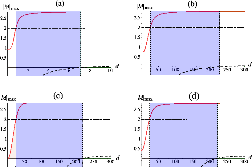
We have shown that the quantum world, where local realism fails, can be revealed by extremely coarse-grained measurements, which is in stark contrast to previous findings [6]. Furthermore, Bell-CHSH inequality can be violated while a Leggett-type inequality imposed by certain non-local realistic theories is satisfied. When $V$ and $d$ take moderate values, the decoherence effects of the type of states under our consideration remain in a reasonable range [22]. A small-scale experimental demonstration of our examples, such as one in Fig. 2(a), may be realized. In this case, the required ETSs become pure entangled coherent states (i.e., $V\sim 1$) with $d\approx 1.1$. Such states can be generated, using a beam splitter, from superpositions of two coherent states with $d\approx 1.6$, which were experimentally demonstrated in a recent experiment [24]. There have been important progresses [25] in obtaining strong nonlinearities, which are demanding yet necessary to implement the local operation $\hat{\cal V}_{j}(\theta_{j})$. Our results unveil unknown aspects of the boundary between quantum and classical worlds and their small-scale experimental realization, although demanding, is foreseeable.

We thank A.C. Doherty, Ph. Grangier and M.S. Kim for discussions. This work was supported by the DTO-funded U.S. Army Research Office (W911NF-05-0397), the ARC, the Queensland State Government, and the KOSEF grant funded by the Korea government (MEST) (R11-2008-095-01000-0). MP is supported by EPSRC (EP/G004579/1).

References

- [1] A. Einstein, B. Podolsky, and N. Rosen, Phys.Rev. 47, 777 (1935).
- [2] J.S. Bell, Physics 1, 195 (1964).
- [3] S.J. Freedman and J.F. Clauser, Phys.Rev.Lett. 28, 938 (1972).
- [4] A. Aspect, Ph. Grangier and G. Roger, Phys.Rev.Lett. 47, 460 (1981).
- [5] W.H. Zurek, Phys. Today 44, 36 (1991); Rev.Mod.Phys. 75, 715 (2003).
- [6] J. Kofler and Č. Brukner, Phys.Rev.Lett. 99, 180403 (2007).
- [7] B.S. Cirel’son, Lett.Math.Phys. 4, 93 (1980).
- [8] T. Paterek et al., Phys.Rev.Lett. 99, 210406 (2007); C. Branciard et al., ibid. 99, 210407 (2007); C. Branciard et al., Nature Phys. 4, 681 (2008).
- [9] A.J. Leggett, Found. Phys. 33, 1469 (2003).
- [10] S. Gröblacher et al., Nature (London) 446, 871 (2007).
- [11] H. Jeong and T.C. Ralph, Phys.Rev.Lett. 97, 100401 (2006); Phys.Rev.A 76, 042103 (2007).
- [12] R. Filip, et al., Phys.Rev.A 65, 043802 (2002); K. Banaszek and K. Wódkiewicz, ibid. 58, 4345 (1998); Z.-B. Chen, et al., Phys.Rev.Lett. 88, 040406 (2002).
- [13] M. Paternostro, H. Jeong, and M.S. Kim, Phys.Rev.A 73, 012338 (2006).
- [14] C.C. Gerry, Phys.Rev.A 59, 4095 (1999).
- [15] H. Jeong, Phys.Rev.A 72, 034305 (2005).
- [16] M. Brune, et al. Phys.Rev.Lett. 77, 4887–4890 (1996).
- [17] B. Yurke and D. Stoler, Phys.Rev.Lett. 57, 13 (1986).
- [18] M. Stobińska, H. Jeong, and T.C. Ralph, Phys.Rev A 75, 052105 (2007).
- [19] J.F. Clauser, et al., Phys.Rev.Lett. 23, 880 (1969).
- [20] D.F. Walls and G.J. Milburn, Quantum Optics (Springer-Verlag, 1994).
- [21] H. Jeong, and M.S. Kim, Phys.Rev.A 65, 042305 (2002).
- [22] H. Jeong, J. Lee, and H. Nha, J.Opt.Soc.Am.B, 25, 1025 (2008).
- [23] For ideal detectors and sufficiently large values of (for given values of ), our approach reproduces the results by Branciard et al. in [8] with a maximal violation of of Leggett’s inequality at .
- [24] A. Ourjoumtsev, et al., Nature (London) 448, 784 (2007).
- [25] L. V. Hau, et al., Nature (London) 397, 594 (1999); P. Bermel, et al., Phys.Rev.Lett. 99, 053601 (2007).