Tensor-entanglement renormalization group approach to 2D quantum systems

Introduction: To obtain various possible quantum phases of a quantum spin system $H=\sum_{\langle ij\rangle}\textbf{\emph{S}}_{i}\cdot\textbf{\emph{J}}_{ij}\cdot\textbf{\emph{S}}_{j}$, we may use a mean-field approach. The mean-field approach can be viewed as a variational approach. For example, to study the possible spin ordered phase of the above quantum spin system, we may start with a trial wave function $|\Psi_{trial}\rangle=\otimes(u_{i}\mid\uparrow\rangle_{i}+v_{i}\mid\downarrow\rangle_{i})$, where $\mid\uparrow\rangle_{i}$ and $\mid\downarrow\rangle_{i}$ are spin states on site $i$. The spin ordered phases can be obtained through minimizing average energy by changing $u_{i}$ and $v_{i}$. But such kind of mean-field theory only apply to states with short-range entanglement (since $|\Psi_{trial}\rangle$ is a direct product state). As a result, we cannot use the traditional mean-field theory to understand quantum phases that have pattern of long-range entanglement (such as topologically ordered states and other quantum states beyond Landau’s symmetry breaking description).[1, 2, 3]

One approach for addressing these phases is to use a more general class of trial wave functions known as “tensor product states” (TPS) or “projected entangled pair states” (PEPS). [4, 5] Tensor product states were first discovered in the context of the (1D) density matrix renormalization group (DMRG) method [6, 7], but were later generalized to higher dimensions and arbitrary lattices. On the square lattice (Fig. 1), the TPS are defined by

where $T_{ejfi}^{m_{1}}$ is a complex tensor with one physical index $m_{i}$ and four inner indices $i,j,k,l,\cdots$. The physical index runs over the number of physical states $d$ on each site and inner indices runs over $D$ values. Unlike simple mean field states, these variational wave functions can describe 2D many-body quantum systems[8] with short-range entanglement (such as symmetry breaking states) as well as long-range entanglement (such as string-net condensed states[9]).

One of main challenges of using this approach in higher dimensions is that it is not easy to compute expectation values in these states. In this Letter, we describe a simple solution to this problem in two dimensions. Our approach - which we call the tensor entanglement renormalization group (TERG) method - is an approximation scheme based on the 2D real space RG method developed in . A different real space RG method can be found in Ref. [11].

As we mentioned earlier, this kind of variational approach has the advantage that it can potentially address 2D quantum many-body states that contain both symmetry breaking orders and topological orders. In this paper, we will just introduce our algorithm by studying a few simple quantum models and compare our results with those obtained through other previous methods. The application of TERG approach to topologically ordered states will be presented in future publications.

To see the efficiency of the TERG method, let us compare it with other variational methods for 2D gapped systems (see Appendix for an explanation):

Here $T$ the calculation time and $\epsilon$ is the achieved accuracy of the calculated average energy for a given many-body state. The acronym VQMC stands for variational Quantum Monte Carlo, while “1D approach” refers to an approximation scheme where one replaces the infinite 2D lattice by an $L\times\infty$ lattice, for $L$ large but finite, and then computes expectation values using a transfer matrix approach.

The TERG method: Let us consider a system with translationally invariant $H=\sum_{i}H_{i}$. $H_{i}$ can always be expressed as a summation of products of local operators: $H_{i}=\hat{O}_{i}^{0}+\hat{O}_{i}^{1}\hat{O}_{j}^{2}+\cdots$. A key step in the variational approach is to calculate the norm and the expectation value of $H_{i}$ for the trial wave function $\Psi(\{m_{i}\})$:

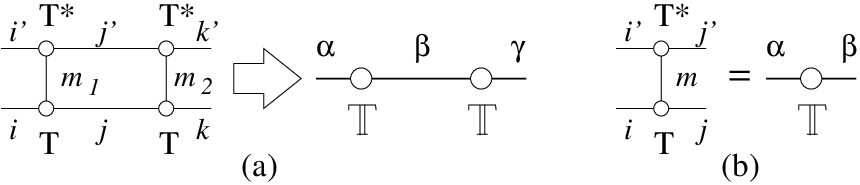
where double-tensors $\mathbb{T}$, $\mathbb{T}^{a}$, $a=0,1,2$, are defined as (see Fig. 2b)

with $O_{mm^{\prime}}^{a}$ the matrix elements of local operators $\hat{O}^{a}$ in the local basis $\left|m\right\rangle$. The tensor-trace (tTr) here means summing over all indices on the connected links of tensor-network (see Fig. 3a). Note that the inner product is obtained from a uniform tensor-network. The average of the on-site interaction is obtained from a tensor-network with one “impurity” tensor $\mathbb{T}^{0}$ at site $i$ (while other site has $\mathbb{T}$). Similarly, for two-body interactions, the tensor-network has two “impurity” tensors $\mathbb{T}^{1}$ and $\mathbb{T}^{2}$ at $i$ and $j$.

Calculating the tensor-trace tTr is an exponentially hard calculation in 2D or higher dimensions. Motivated by the tensor-renormalization approach developed in Ref. [10], we can accelerate the calculation exponentially if we are willing to make an approximation. The basic idea is quite simple and is illustrated in Fig. 3. After finding the reduced double-tensor $\mathbb{T}^{\prime\prime}$, we can express $\text{tTr}[\mathbb{T}\otimes\mathbb{T}\cdots]\approx\text{tTr}[\mathbb{T}^{\prime\prime}\otimes\mathbb{T}^{\prime\prime}\cdots]$ where the second tensor-trace only contain a quarter of the double-tensors in the first tensor-trace. We may repeat the procedure until there are only a few double-tensor in the tensor-trace. This allows us to reduce the exponential long calculation to a polynomial long calculation.

The detail implementation of the above TERG approach is actually a little more involved. For an uniform tensor-network Fig 3a, we can coarse grain it in two steps. The first step is decomposing the rank-four tensor into two rank-three tensors. We do it in two different ways on the sublattice purple and green (see Fig. 4a). On purple sublattice, we have $\mathbb{T}_{\alpha\beta\mu\nu}=\sum_{\gamma^{\prime}}{S_{1}}_{\mu\nu\gamma^{\prime}}{S_{3}}_{\alpha\beta\gamma^{\prime}}$ and on green sublattice, we have $\mathbb{T}_{\alpha\beta\mu\nu}=\sum_{\gamma^{\prime}}{S_{2}}_{\nu\alpha\gamma^{\prime}}{S_{4}}_{\beta\mu\gamma^{\prime}}$. Note that $\alpha,\beta,\mu,\nu$ run over $D^{2}$ values while $\gamma^{\prime}$ run over $D^{4}$ values.

Next we try to reduce the range of $\gamma^{\prime}$ through an approximation.[10] Say, on purple sublattice, we view $\mathbb{T}_{\alpha\beta\mu\nu}$ as a matrix $M_{\alpha\beta;\mu\nu}^{\rm{red}}=\mathbb{T}_{\alpha\beta\mu\nu}$ and do singular value decomposition $M^{\rm{red}}=U\Lambda V^{\dagger}$. We then keep only the largest $D_{cut}$ singular values $\lambda_{\gamma}$ and define ${S_{1}}_{\mu\nu\gamma}=\sqrt{\lambda_{\gamma}}V^{\dagger}_{\gamma,\mu\nu}$, ${S_{3}}_{\alpha\beta\gamma}=\sqrt{\lambda_{\gamma}}U_{\alpha\beta,\gamma}$. Thus, we can approximately express $\mathbb{T}_{\alpha\beta\mu\nu}$ by two rank-three tensors $S_{1}$, $S_{3}$

Similarly, on green sublattice we may also define $\mathbb{T}_{\alpha\beta\mu\nu}$ as a matrix $M_{\nu\alpha;\beta\mu}^{\rm{green}}$ and do singular value decompositions, keep the largest $D_{\text{cut}}$ singular values and approximately express $\mathbb{T}_{\alpha\beta\mu\nu}$ by two rank three tensors $S_{2},S_{4}$.

After such decompositions, the square lattice is deformed into the form in Fig. 4b (see also Fig. 5). The second step is simply contract the square and get a new tensor on the coarse grained lattice.

The range of indices for the reduced double-tensor $\mathbb{T}^{\prime}$ is only $D_{\text{cut}}$ which can be chosen to be $D^{2}$ or some other values. Repeat the above two steps twice, we can get the reduction from Fig. 3a to 3c.

The above TERG procedure can be easily generalized to tensor-network with “impurities”, such as the one in Fig. 5 which has four “impurity” tensors. Evaluating Fig. 5 will allow us to calculate the averages of up to four-body nearest-neighbor interactions (which include on-site interaction, nearest-neighbor and next-nearest-neighbor two-body interactions). TERG procedure is illustrated in Fig. 5. We note that the number and the relative positions of “impurity” tensors do not change after each iteration. So we repeat the same iterative calculation until there are only a few tensors in the tensor-trace. Thus the calculations of the averages of local operators is also reduced to polynomial long calculations. The total computational complexity is $\text{cost time}\sim D_{\text{cut}}^{6}\text{log}N$ on square lattice ($N$ is the total number of sites). For gapped systems in the thermodynamic limit, the truncation error can be estimated as $\epsilon\sim\exp\left[-\text{const}\cdot\left(\log D_{\text{cut}}\right)^{2}\right]$[10]. After calculating the inner product and the average of $H_{i}$ in (2), we can obtain the approximated ground state with minimized average energy by adjusting the elements in the tensor $T$.

Examples: To test our TERG algorithm, we first calculate ground state and its magnetization along $x$ and $z$ directions for the transverse field Ising model:

We choose the tensor $T$ in Eq. (1) to be real and has 90 degree rotational symmetry. We also choose the inner dimension $D=2$ and keep 18 singular values at each iteration ($D_{\text{cut}}=18$). The total system size is up to $2^{9}\times 2^{9}$ sites. The average energy for a tensor $T$ is calculated using the TERG approach. We use Powell minimization method to find the minimal average energy and the corresponding tensor which gives us the variational ground state.

In Fig. 6 we plot the polarization along $x$ direction and $z$ direction in the variational ground state. We note that despite the $\sigma^{z}\to-\sigma^{z}$ symmetry in the Hamiltonian, the tensor $T$ that minimize the average energy may break the $\sigma^{z}\to-\sigma^{z}$ symmetry and give rise to non-zero polarization in $z$ direction. We find a second order phase transition at $h_{c}\approx 3.08$. We further fit the critical exponent

with $\beta\approx 0.333\pm 0.003$. Both the values of critical field and critical exponent $\beta$ here are very close to the QMC results, with $h^{QMC}_{c}\simeq 3.044$[12] and $\beta^{QMC}\simeq 0.327$[13]. They are much better than the meanfield results $h_{c}=4$ and $\beta=0.5$.

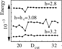
To see the truncation error caused by $D_{cut}$, we plot the ground state energy (per site) of Eq. 7 as a function of $D_{cut}$, for $h=2.8,3.2$, and $h=h_{c}=3.08$ (see Fig. 7). The energies for different $h$’s are shifted by different constants so that the three curves can be fitted into one window. Notice that for off critical systems ($h=2.8,3.2$), the energy converges very quickly for small $D_{cut}$ ($\sim 26$). Even at the critical point $h=h_{c}=3.08$, the error in energy per site is of order $10^{-4}$. The truncation error is much smaller for gapped off-critical states.

As another more stringent test, we also apply the TERG method to study Heisenberg model $H=\sum_{\langle ij\rangle}\textbf{\emph{S}}_{i}\cdot\textbf{\emph{S}}_{j}$ on square lattice which contains gapless excitations. Again we choose $D=2$, $D_{cut}=18$ and total system size $2^{9}\times 2^{9}$ sites. We choose tensors $T_{A}$ and $T_{B}$ to be real and has 90 degree rotational symmetry on sublattice $A$ and $B$. We find the ground state energy to be $-0.33$ per bond, which is quite close to the best QMC results(-0.3350).[14] The TERG method also allows us to calculate correlation function using tensor-network with two “impurity” tensors with arbitrary separations. Through the long-range correlation function, we find that the total magnetization is $m=\sqrt{\langle S_{i}^{x}S_{j}^{x}+S_{i}^{y}S_{j}^{y}+S_{i}^{z}S_{j}^{z}\rangle}=0.39$, which is larger than the QMC results(0.307).[14] We see that a small error in ground state energy (which depends only on short-range correlation) can leads to a larger error on correlations at long distances.

Conclusions and discussions: The TERG approach is a simple generic method to obtain various quantum phases and quantum phase transitions for quantum systems in any dimension. The most important feature of TERG approach is that it can handle quantum states with long-range entanglement (such as topologically ordered states). When we use traditional mean-field theory to calculate quantum phase diagram, the topological ordered phases cannot appear in such a mean-field phase diagram, since the mean-field states are limited to those with short-range entanglement. The TERG approach solves this problem and can generate phase diagrams that contain both symmetry breaking states and topologically ordered states.

Acknowledgements: We would like to thank Frank Verstraete for very helpful discussions and comments. This research is supported by the Foundational Questions Institute (FQXi) and NSF Grant DMR-0706078.

Appendix: In a VQMC calculation, the error $\epsilon$ is a statistical error that scales like $1/N^{1/2}$ where $N$ is the number of samples. The computational time $T$ scales like $N$. Thus the scaling of the error with computational time is given by $\epsilon\sim 1/T^{1/2}$.

In the 1D approach, the error $\epsilon$ is a finite size error that comes from the truncation of the infinite 2D lattice to an $L\times\infty$ lattice. In a gapped system we expect this error to fall off as $e^{-L/\xi}$ where $\xi$ is the correlational length. On the other hand, the computational time $T$ is exponential in $L$ since the method requires diagonalizing a transfer matrix whose size is exponentially large in $L$. We conclude that the error scales with computational time as $\epsilon\sim e^{-\text{const.}\cdot\log T}$.

In the TERG approach, the truncation error for each iteration step scales as $\epsilon_{1}\sim e^{-\text{const.}\cdot(\log D_{\text{cut}})^{2}}$, since calculating the norm and averages is like calculating the partition function in . The total truncation error for a system of size $L$ is $\epsilon_{t}\sim(\log L)e^{-\text{const.}\cdot(\log D_{\text{cut}})^{2}}$ since such a system requires $\log L$ iterations. On the other hand, the finite size error is $\epsilon_{s}\sim e^{-L/\xi}$. Minimizing the sum of the two errors, we see that the optimal $L$ is given by $L\sim(\log D_{\text{cut}})^{2}$. Since the computational time scales polynomially in $D_{\text{cut}}$, we conclude that the total error scales like $\epsilon\sim e^{-\text{const.}\cdot(\log T)^{2}}$ (neglecting subleading log corrections).

References

- [1] X.-G. Wen, Physics Letters A 300, 175 (2002).
- [2] A. Kitaev and J. Preskill, Phys. Rev. Lett. 96, 110404 (2006).
- [3] M. Levin and X.-G. Wen, Phys. Rev. Lett. 96, 110405 (2006).
- [4] F. Verstraete and J. I. Cirac, cond-mat/0407066.
- [5] F. Verstraete, M. M. Wolf, D. Perez-Garcia, and J. I. Cirac, Phys. Rev. Lett. 96, 220601 (2006).
- [6] S. R. White, Phys. Rev. Lett. 69, 2863 (1992).
- [7] S. stlund and S. Rommer, Phys. Rev. Lett. 75, 3537 (1995).
- [8] J. Jordan, R. Or¨²s, G. Vidal, F. Verstraete, and J. I. Cirac, cond-mat/0703788.
- [9] Z.-C. Gu, M. Levin, B. Swingle, and X.-G. Wen.
- [10] M. Levin and C. P. Nave, Phys. Rev. Lett. 99, 120601 (2007).
- [11] G. Vidal Phys. Rev. Lett. 99, 2204005 (2007).
- [12] H. W. J. Blote and Y. Deng, Phys. Rev. E 66, 066110 (2002).
- [13] A. Pelissetto and E. Vicari, Phys. Rept. 368, 547 (2002).
- [14] A. W. Sandvik, Phys. Rev. B 56, 11678 (1997).