Vol.0 (200x) No.0, 000–000
A Super-high Angular Resolution Principle for Coded-mask X-ray Imaging Beyond the Diffraction Limit of Single Pinhole
Abstract
High angular resolution X-ray imaging is always demanded by astrophysics and solar physics, which can be realized by coded-mask imaging with very long mask-detector distance in principle. Previously the diffraction-interference effect has been thought to degrade coded-mask imaging performance dramatically at low energy end with very long mask-detector distance. In this work the diffraction-interference effect is described with numerical calculations, and the diffraction-interference cross correlation reconstruction method (DICC) is developed in order to overcome the imaging performance degradation. Based on the DICC, a super-high angular resolution principle (SHARP) for coded-mask X-ray imaging is proposed. The feasibility of coded mask imaging beyond the diffraction limit of single pinhole is demonstrated with simulations. With the specification that the mask element size of and the mask-detector distance of 50 m, the achieved angular resolution is 0.32 arcsec above about 10 keV, and 0.36 arcsec at 1.24 keV ( nm) where diffraction can not be neglected. The on-axis source location accuracy is better than 0.02 arcsec. Potential applications for solar observations and wide-field X-ray monitors are also shortly discussed.
keywords
instrumentation: high angular resolution—techniques: image processing—telescopes1 Introduction
High angular resolution X-ray imaging is always demanded by astrophysics and solar physics, for example to study black holes near event horizon, relativistic jets of super massive black holes, as well as solar flares and coronal activities. So far the best imaging technology for X-ray observation is realized by grazing incidence reflection (Aschenbach [1985]), which provides a very good angular resolution, for example down to 0.5 arcsec as in the case of the Chandra X-ray Observatory (Weisskopf et al. [2000]). The diffraction limit of Chandra is about 8 miliarcsec at 6 keV; however slope errors and other surface irregularities that affect the angle of reflection prevent the angular resolution better than 0.5 arcsec. Further more, the grazing incidence reflection is limited by the working energy band, which hardly exceeds tens of keV. A possible way to improve the angular resolution beyond Chandra’s requires a different technology, for example the diffractive-refractive X-ray optics proposed by Gorenstein ([2007]) or the Fourier-Transform imaging by Prince et al. ([1988]). As an alternative, a super-high angular resolution principle (SHARP) for a coded-mask X-ray imaging telescope concept is proposed here.
The coded mask imaging technology, which has been reviewed by Zand ([1996]), is widely applied for X-ray observations, for example the INTEGRAL mission (Winkler et al. [2003]) of ESA and the SWIFT mission (Gehrels [2004]) of NASA. Both missions have angular resolution in tens of arcmin, since the distances between the masks and the detectors are limited by the dimensions of the satellites. In principle super-high angular resolution better than Chandra can be achieved by a coded-mask telescope with sub-millimeter size of mask pinholes and long mask-detector distances, which can be tens, even hundreds of meters with the formation-flying technology (for example proposed for XEUS (ESA [2001]) of ESA) or the mast technology (for example applied in Polar mission of NASA). The X-ray diffraction effect in a coded-mask system has been commonly thought to be negligible due to high photon energies in hard X-ray and gamma-ray range as well as relatively small mask-detector distance. Whereas for coded-mask telescope with a super high angular resolution in the milli-arc-second range, the X-ray diffraction effect could not be neglected, especially at low energy end (in the range of several keV), which might degrade the imaging performance remarkably, as pointed out by Prince et al. ([1988]) and Skinner ([2004]). In this work, we study the diffraction effect in SHARP with numerical computations, and propose a diffraction-interference cross correlation reconstruction method and demonstrate the feasibility of coded mask imaging beyond the diffraction limit of single pinhole. A potential application for solar observations is also shortly discussed.
2 The coded-mask principle and diffraction-interference reconstruction
2.1 The coded-mask principle and SHARP
In the limit of geometrical optics, i.e., the diffraction effect is not considered, the basic concept of coded-mask imaging is shown in Fig. 1. The coded-mask camera has a mask on top of a position-sensitive detector with a mask-detector distance . Two point sources project the mask pattern onto the detector plane. The shift and the strength of projections encode the position and the flux of sources separately. The detection of the X-ray flux can be described with Equ. 1 (Fenimore et al. [1978]),
| (1) |
where is the X-ray flux spatial distribution, is the encoding pattern of mask and means cross correlation. For the commonly applied cross correlation method, a matrix is used for reconstruction, as shown in Equ. 2,
| (2) |
where is the estimation of X-ray flux spatial distribution, if is a function. The encoding pattern is often chosen so that its auto-correlation function is a function. Therefore is commonly applied. The width of the Point Spread Function (PSF) obtained with Equ. 2 is defined as ( is the size of the mask element). The cyclic optimal coded-mask configuration (Zand [1996]) is also employed here. The coded mask or the mask pattern consisted of four basic patterns is about four times the size of the detector, and one basic pattern cyclically extends about twice along the width and length directions of the mask. In the next sections, simulations are done with the following assumptions: the basic pattern is totally random; the detector pixel size is equal to the mask element size, both of which are in square shape; the mask and the detector are assumed to be idealized, i.e., the mask has no thickness, the opaque mask elements block the X-ray completely and one incident event can only be recorded in one detector pixel.

In this work, and are chosen to be the basic parameters for the simulations of SHARP, which means in sub-arcsec range. Since the simulations employ two dimensional FFT (please refer to Sec. 2.2) which requires tremendous computing resources, the basic pattern simulated contains only elements, i.e., the reconstructed image contains the same pixels and each pixel is . The fully coded Field-Of-View (FOV) is .
2.2 The diffraction-interference cross correlation method
As shown in Fig. 2, is the mask modulation function, which is 1 or 0 with idealized mask. is a vector from point on the mask to the on the detector. is the wave vector. Since there are many pinholes in the mask, both diffraction and interference will take place on the detector plane. The diffraction-interference is described with Fresnel-Huygens principle (Lindsey [1978]) as,
| (3) |
where is the amplitude distribution of incident photons, which is described with the plane wave in our case as . The flux distribution is proportional to . is constant. In our case the dimension of the mask is far less than the mask-detector distance , we have . Therefore Equ. 3 becomes
| (4) |
where , , , . Equ. 4 is the Fourier transform approximation of Fresnel-Huygens principle, which can be simulated with an FFT algorithm. The conditions for the validity of this approximation are discussed by Lindsey ([1978]), and are satisfied in our simulations.

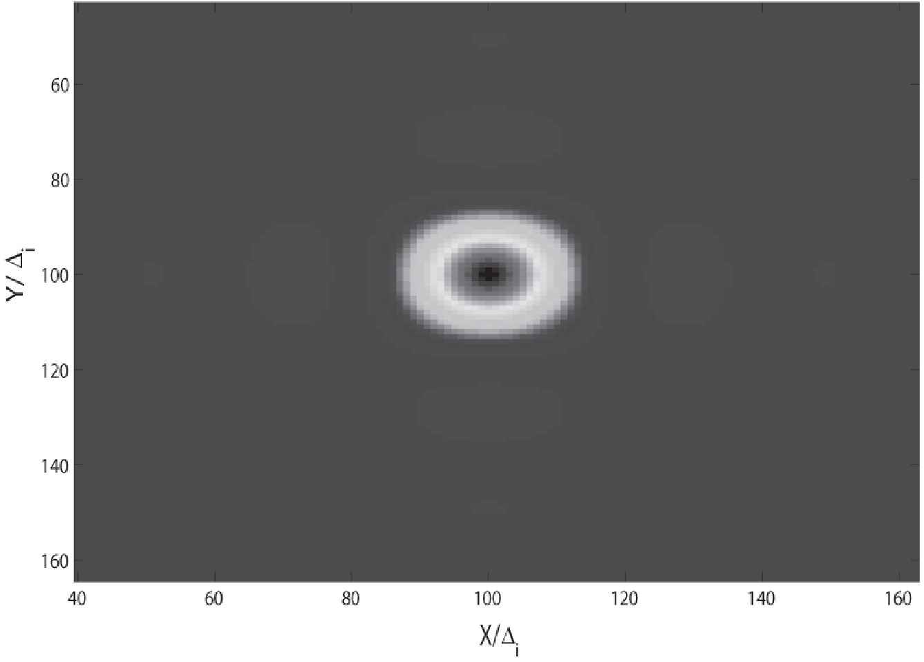
The X-ray diffraction can not be neglected at the low energy end as in Fig. 3, which shows the simulated flux distribution on the detector plane with a square pinhole in front of it (50 m away) for 1.24 keV photons ( nm). The flux spreads much larger than (each pixel in Fig. 3 is ) due to the diffraction effect.
If the reconstruction matrix in the cross correlation method is still chosen to be equal to (so-called geometrical reconstruction matrix, which is indicated as ) at the low energy end, the diffraction effect would degrade the reconstructed image remarkably. Fig. 4a shows the reconstructed image of a monochromatic on-axis point source () obtained by geometrical matrix. The reconstructed image is normalized so that the total integral flux is one photon, and all the reconstructed images in this work are normalized in the same way if not specified. The point source is hardly identified with the Fresnel diffraction stripes clearly observed. Since the X-ray probability wave through different mask open elements interferes with each other, the mask spatial information should be encoded into the diffraction-interference pattern on the detector. We then choose the reconstruction matrix at certain energy as the normal incident diffraction-interference pattern (so-called diffraction-interference matrix, which is indicated as ) on the detector plane. Fig. 4b shows the reconstructed image obtained with of the same source in Fig. 4a, and the point source can be clearly identified although slight Fresnel stripes still exist. This new reconstruction method is called diffraction-interference cross correlation method (DICC), which can be described with Equ. 5,
| (5) |
can be obtained by numerical simulation as shown in Equ. 4 or from actual measurements. The angular resolution of DICC is beyond the single pinhole (the single mask open element) diffraction limit as indicated in Fig. 4.

3 The simulation results
We have simulated the reconstructed images at several energies from 1.24 keV ( nm) to 6.2 keV ( nm), where DICC is valid. To illustrate the main properties of this method, we mainly discuss the imaging performance of DICC around 1 nm, which is also compared with that in the limit of geometrical optics.
3.1 Angular resolution
We calculate the reconstructed image of two point sources with the same flux (Poisson fluctuations are not considered here). The angular resolution is defined as the minimum angular distance between these two sources, which can be separated by the 50% contour line of the maximum flux on the reconstructed image. Fig. 5a shows the reconstructed images in the limit of geometrical optics for two point sources with angular distance ; the two sources can not be separated. However in Fig 5b two sources with angular distance can just be separated. Therefore the angular resolution is 0.32 arcsec in the limit of geometrical optics, i.e., at high energy end (above about 10 keV) with diffraction negligible. With the same procedure, the angular resolution of DICC for nm photons is obtained as 0.36 arcsec, i.e., the two sources can not be separated in Fig. 5c, but can be separated in Fig. 5d. This means the diffraction effect degrades the angular resolution by only about 12.5%, a significant improved compared to that in Fig. 3. We also calculated the reconstructed images with DICC for nm point sources at different locations inside the FOV, but no observable reconstruction degradation is found compared with the on-axis source case.

3.2 Source location accuracy
The reconstructed images for an on-axis point source is simulated 10000 times with 1000 photons recorded (Poisson fluctuations are considered). The source location of each simulation is calculated by fitting the reconstructed image to the PSF. The calculated source location distribution with DICC for nm is shown in Fig. 6a, which is concentrated within . The same simulation is also done in the limit of geometrical optics, which is shown in Fig. 6b. Therefore the source location accuracy is better than for 1000 detected photons.

3.3 System constraints
Since the diffraction pattern on the detector plane is energy dependent, the diffraction matrix is also energy dependent. In practice the detector can not identify two photons with an energy difference within the detector’s spectroscopy resolution, i.e., in practice photons within a small energy band must share a common diffraction matrix. Fig. 7 shows the reconstructed images of several on-axis point sources with wavelengths around 1 nm, which all apply the diffraction matrix of 1 nm photons (marked as ). The point source can be clearly identified. Obviously the imaging qualities are degraded by applying the instead of their own diffraction matrixes. Tab. 1 gives the angular resolution at several wavelengths around 1 nm by applying as reconstruction matrix instead of their own. For the 1.05 nm on-axis source, the angular resolution is degraded to by applying .
| Wavelength (nm) | 0.95 | 0.97 | 0.99 | 1 | 1.01 | 1.03 | 1.05 |
|---|---|---|---|---|---|---|---|
| Angular resolution (arcsec) | 0.39 | 0.38 | 0.37 | 0.36 | 0.37 | 0.39 | 0.41 |
Based on the detector energy resolution, the system constraint is considered. Assuming the detector pixel size , the difference of the main diffraction stripe diameters of photons with wavelength difference is
| (6) |
If the spectroscopy resolution of the detector is , spatially the detector does not need to distinguish for photons with wavelength difference ,
| (7) |
Here is a constant and depends upon the mask open fraction. For a 50% open mask, our simulations indicates that . For a mask fraction much less than 50%, is possible. Then with known basic parameters, i.e., and , the requirement for detector spectroscopy resolution is
| (8) |
In practice and are chosen to match the detector performance, which means
| (9) |
or
| (10) |
Therefore the larger the is, the more compact the system can be. Here is chosen for convenience, with which nm, and m satisfies the system constraint. The spectroscopy resolution 0.05 nm requires about 120 eV energy resolution @ nm, which can be provided by modern silicon imaging detectors like CCD or DEPFET (Strüder [2000]).

4 Discussion and Conclusion
By applying DICC, the system angular resolution is no more limited by single pinhole diffraction limit at low energy end, but limited by detector spectroscopy performance. Tab. 2 shows a brief comparison of SHARP with several X-ray astronomy missions. The advantage of SHARP is quite obvious: excellent angular resolution and easily fabricated mask which does not require high accuracy mechanical fabrication of X-ray grazing lens. However the detector effective area of a coded-mask telescope is smaller than the its actual area due to the encoding pattern. Further more each detector pixel receives background photons from all over the FOV. Therefore the sensitivity is limited by its large background and small effective area compared with that in the grazing incidence reflection case.
Current detector technology can provide even better energy resolution than 0.05 nm @1 nm, which means the angular resolution discussed above can be improved further by increasing the mask-detector distance as indicated in Equ. 10 or by decreasing the mask element size as indicated in Equ. 9. For example for a detector with 0.002 nm spectroscopy resolution (5 eV @ 1 keV), and m satisfies the system constraint with .
A potential application of SHARP will be the solar observation at 1-100 keV energy band with sub-arcsec angular resolution. The main objectives may be the coronal mass ejection (CME) and solar flares, including fine structures and evolutions of the solar flares, nonlinear solar flare dynamics, solar particle acceleration mechanism et al. Therefore applications of SHARP are foreseen to make significant progress on the study of solar high energy explosive events and the space weather forecast model. Another potential application is to make wide-field X-ray monitors with SHARP; its sub-arc angular resolution may allow the counterparts of gamma-ray bursts, X-ray bursts, black hole and neutron star transients to be identified without the requirement of subsequent follow-up observations of focusing X-ray telescopes.
| Mission | SHARP | Chandra | Integral11 1 IBIS onboard | RHESSI | Hinode (Solar B)22 2 XRT onboard |
|---|---|---|---|---|---|
| Imaging technology | Coded-mask | Focusing | Coded-mask | Rotation Modulation & Fourier Transform | Focusing |
| Energy band | 1-100 keV | Up to 10 keV | 15 keV-10 MeV | 3-150 keV33 3 The upper layer | About to 6 keV |
| Energy resolution | 133 eV@5.9 keV44 4 Take DEPFET as focal plane detector (Treis et al. [2006]) | ACIS: about 148 eV@5.9 keV55 5 CCD S3 on board | 9 % @ 100 keV | keV66 6 Below 100 keV | eV @5.9 keV77 7 Calculated based on the ENC el. |
| Angular resolution | 0.32-0.36 arcsec | 0.5 arcsec88 8 On-axis point source | 12 arcmin | 2.26 arcsec99 9 The collimator # 1 | 2 arcsec @ 0.523keV1010 10 68% source flux within 2 arcsec |
Acknowledgements.
We thank C. Fang, W. Q. Gan, J. Y. Hu, Z. G. Dai, X. D. Li, Y. F. Huang and X. Y. Wang for many interesting discussions and suggestions on SHARP and its potential applications. We are grateful to the anonymous referee for providing valuable comments and suggestions promptly. SNZ acknowledges partial funding support by the Ministry of Education of China, Directional Research Project of the Chinese Academy of Sciences under project No. KJCX2-YW-T03 and by the National Natural Science Foundation of China under grant Nos. 10521001, 10733010, 10725313 and 10327301.References
- [1985] Aschenbach B., 1985, Reports on Progress in Physics, 48 (5): 579-629
- [1978] Fenimore E. E., Cannon T. M., 1978, Applied Optics, 17: 337-347
- [2004] Gehrels N., 2004, New Astronomy Reviews, 48, 431-435
- [2007] Gorenstein P., 2007, Advances in Space Research, 40 (8): 1276-1280
- [1978] Lindsey C. A., 1978, J. Opt. Soc. Am., 68 (12): 1708
- [1988] Prince T. A., Hurford G. J., Hudson H. S., Crannell C. J., 1988, Solar Physics, 118: 269-290
- [2004] Skinner G. K., 2004, New Astronomy Reviews, 48: 205-208
- [2000] Strüder L., 2000, Nucl. Instr. and Meth. A, 454 (1): 73-113
- [2001] The XEUS Telescope Working Group, 2001, X-ray evolving universe spectroscopy-the XEUS telescope, ESA SP-1253
- [2006] Treis J., Fischer P., Halker O. et al., 2006, Nucl. Instr. and Meth. A, 568 (1): 191-200
- [2000] Weisskopf M. C., Tananbaum H. D., Van Speybroeck L. P., O’Dell S. L., 2000, In: J. Truemper, B. Aschenbach, eds., Proceedings of SPIE, 4012, p. 2
- [2003] Winkler C., Courvoisier T. J.-L., Cocco G. D. et al., 2003, A&A, 411, L1
- [1996] Zand J., 1992, 1996, Coded aperture camera imaging concept [EB/OL], http://lheawww.gsfc.nasa.gov/docs/cai/coded.html