Resistive jet simulations extending radially self-similar magnetohydrodynamic models
Abstract
Numerical simulations with self-similar initial and boundary conditions provide a link between theoretical and numerical investigations of jet dynamics. We perform axisymmetric resistive magnetohydrodynamic (MHD) simulations for a generalised solution of the Blandford & Payne type, and compare them with the corresponding analytical and numerical ideal-MHD solutions. We disentangle the effects of the numerical and physical diffusivity. The latter could occur in outflows above an accretion disk, being transferred from the underlying disk into the disk corona by MHD turbulence (anomalous turbulent diffusivity), or as a result of ambipolar diffusion in partially ionized flows. We conclude that while the classical magnetic Reynolds number measures the importance of resistive effects in the induction equation, a new introduced number, with the plasma beta, measures the importance of the resistive effects in the energy equation. Thus, in magnetised jets with , when resistive effects are non-negligible and affect mostly the energy equation. The presented simulations indeed show that for a range of magnetic diffusivities corresponding to the flow remains close to the ideal-MHD self-similar solution.
Keywords:
stars: pre–main sequence – magnetic fields – MHD – ISM: jets and outflows1 Introduction
Collimated outflows of plasma observed to emerge from the vicinity of a wide spectrum of cosmic objects are still a challenge for observational and theoretical astrophysics. These outflows play a key role in the transport of angular momentum and energy of the accreted gas facilitating thus, for example, star formation. Nevertheless, when new observations put more and more severe constraints on models, these seem to be still too rudimentary to provide sophisticated answers.
The starting point of the modeling of jets are the ideal MHD equations, which can be solved analytically by assuming axisymmetry, time-independence and the self-similarity ansatz. Analytical models of ideal MHD disk winds (Blandford & Payne 1982, re-visited in Vlahakis et al. 2000; hereafter V00), provide not only the first insight into the physics of such outflows but equally important they can be used as a test bed of more sophisticated simulations of the resistive MHD system via various numerical codes. In Vlahakis & Tsinganos (1998) general classes of self-consistent ideal-MHD solutions have been constructed. Two sets of exact MHD outflow models have been found: meridionally and radially self-similar ones. Previously known studies were recognised to belong in this more general classification of all available analytical models. In particular, the V00 study remedied the physically unacceptable feature of the Blandford & Payne (1982) terminal wind solution which was not causally disconnected from the disk (see also Ferreira & Casse (2004) when a resistive disk is included).
Among the basic problems which still remained to be solved however were the common deficiency that all radially self-similar models had, namely, a cut-off of the solution at small cylindrical radii and also at some finite height above the disk where they were unphysical. The reason for such behaviour is a strong Lorentz force close to the system’s axis. The invalid analytical solution very close to the axis has been corrected numerically. Also, a search in the numerical simulations for solutions at larger distances from the disk has been performed, in Gracia et al. (2006; hereafter GVT06), where ideal-MHD numerical simulations with the V00 solution as initial condition have been performed using the NIRVANA code (version 2.0, Ziegler 1998). These results have been verified also by using the PLUTO code (Mignone et al. 2007) in the ideal MHD simulations by Matsakos et al. (2008).

The next step in the exploitation of the available analytical solutions has been the investigation of the dynamical connection of the outflow to the underlying disk (see e.g., Königl, 1989; Wardle & Königl 1993; Li 1995; Ferreira 1997; Casse & Keppens 2004; Zanni et al. 2007), providing some understanding of the formation of jets from the accretion disk. At the same time, since the disk is naturally resistive, the need emerged to go beyond the ideal MHD regime. With the magnetic field included, the effects of the magnetic resistivity, both numerical and physical, had to be addressed, discriminated and analysed.
In fully ionized disks an anomalous turbulent diffusivity has to be invoked to allow for accretion of matter crossing a large-scale magnetic field. This anomalous turbulent diffusivity may be present in the outflow as well, at least at distances close to the disk. In partially ionized disks the physical conductivity is properly described by a tensor, consisting of three distinct parts corresponding to the ambipolar diffusion, the Hall effect, and the Ohmic dissipation (e.g. Wardle & Ng, 1999; Salmeron et al., 2007). The dominant mechanism in the outflow above the disk is most likely the ambipolar diffusion (e.g., Sano & Stone 2002; Kunz & Balbus 2004; Wardle 2007), and can be appropriately described only by a multifluid MHD. Nevertheless, in both cases (turbulent or ambipolar diffusion), a scalar conductivity can capture the basic characteristics of the breakdown of ideal MHD related to the magnetic field diffusion and the resistive heating.
The effects of the resistive heating in the formation and acceleration of jets from resistive disks or tori, have been studied in Kuwabara et al. (2000, 2005), concluding that Joule heating is not playing an essential role in jet formation. However, in these studies only low values (lower than the critical value that we define below) of resistivity were examined. Resistive effects have been also studied in Fendt & Čemeljić (2002; hereafter FC02). In this case, however, the energy equation was not solved and a polytropic equation of state has been assumed instead, such that the effects of finite resistivity have not been directly incorporated in the energetics of the problem. Safier (1993a) working in the ambipolar diffusion regime of outflows associated with young stars, found that the diffusive term in the energy equation cannot be neglected. The heating of the gas could have significant observational consequences (see e.g. Safier 1993b; Martin 1996b; Cabrit et al., 1999; Garcia et al., 2001a,b; O’Brien et al., 2003; Shang et al., 2004). Safier’s (1993a) work also shows why the cooling term in the energy equation and the ionization balance equation need to be considered in a full investigation. He was able to uncover a strong feedback mechanism between the gas temperature and the ionization fraction (which scales inversely with the ambipolar diffusion heating rate). The result of the heating depends also on the geometry of the flow which strongly affects the adiabatic cooling. In a spherical outflow this cooling effectively counters the Joule dissipation heating (Ruden et al., 1999), while in a disk-driven jet with a small streamline divergence the adiabatic cooling is relatively unimportant (at least initially). Interestingly, Joule dissipation can play a role (although generally not a dominant one) also in magnetically guided accretion problems (e.g., Martin 1996a).
Numerical resistivity is implicitly present in any numerical simulation, and its various effects need to be identified and studied in detail. This is one of the main aims of this paper. The other one is to investigate the effects of small physical resistivity, examine the stability of the resistive jet solutions and define when the resistivity is ”small” and when it becomes ”large”. The novel approach followed here is that the analytical solution is a stationary reference solution, something which was lacking in the previous investigations of resistive MHD flows, e.g. FC02.
The structure of the paper is as follows. The analytical expressions and their modification in the setup for numerical simulations are first presented in Sec. 2. Then the resistive-MHD solutions (Sec. 4) are systematically compared to the ideal-MHD ones of Sec. 3. In Sec. 5 we introduce an extension of the magnetic Reynolds number which quantifies the transition from an ideal-like behaviour of the low diffusivity solutions for values of the diffusivity below a critical value , to a transient and erratic behaviour of the solutions for . The main possible consequences for astrophysical outflows are briefly discussed. A summary of the main results is given in the last Sec. 6.
2 Problem setup
2.1 Governing equations
The resistive-MHD equations solved by the NIRVANA code are, in SI units:
| (1) | |||
| (2) | |||
| (3) | |||
| (4) | |||
| (5) |
where is the flow velocity, is the magnetic field, are the gas density and pressure, and is the gravitational potential of the central mass . The internal energy (per unit mass) is related to the pressure and density by
| (6) |
where is the effective polytropic index. The magnetic diffusivity is assumed constant and is related to the resistivity , where is the permeability of vacuum.
2.2 Initial and boundary conditions
For the initial and boundary conditions of the simulations the self-similar solution of V00 is used. The assumptions of steady-state, axisymmetry and radial self-similarity result in the following expressions for the physical quantities in spherical (, , ) and cylindrical (, , ) coordinates:
| (7) | |||
| (8) | |||
| (9) | |||
| (10) | |||
| (11) | |||
| (12) |
where , are functions of , and
| (13) |
Here we decomposed vector quantities in poloidal (index ) and toroidal (index ) components. We set the solution parameters to , as in the V00 solution.
The diffusivity (which is assumed constant throughout the domain) is normalised as , with dimensionless.


The self-similar solution breaks down near the rotation axis. This becomes evident from the fact that all physical quantities are proportional to a power of the function , which is divergent on the axis (), see Eqs. (7-12). In addition, the analytical solution of V00 is not provided for smaller than 0.025 rad, measured from the axis.
To perform numerical simulations in a computational box with the symmetry axis included, we need to modify/extrapolate the analytical solution. Near the axis, we extrapolated the missing analytical solutions for the tabulated functions , and , as described in GVT06. A similar result can be achieved with less involved extrapolation, as shown in Matsakos et al. (2008). Modification of the functions G and M means also that the pressure/energy is modified near the axis.
For the magnetic field in the vicinity of the symmetry axis there is an additional problem. With the extrapolated functions and the magnetic field as given by Eq. (9) is not divergence-free. This leads to the need for suitable modification of the initial magnetic field. A simple modification is to compute the component from the component of the self-similar expression
| (14) |
and subsequently the radial component by solving the with boundary condition .


The poloidal velocity field should, in result, also be modified. Initially , as demanded for steady ideal-MHD flow. Therefore, we compute the new poloidal velocity field, maintaining the magnitude of velocity, but correcting the direction so that holds.
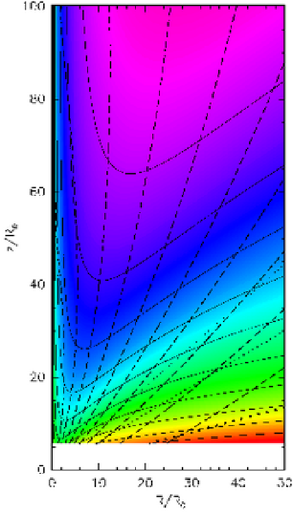
The modified initial magnetic field is presented in Fig. 1, together with the modified density isocontours and positions of the critical surfaces.
For boundary conditions we use symmetry conditions on the rotation axis, and outflow conditions on the outer and boundaries. On the lower boundary (we take in all simulations) we fix the values for six physical quantities, namely density, three velocity components, the azimuthal and one poloidal magnetic field component (the other one is given from ). The pressure/internal energy boundary condition is kept fixed only in the super-sonic region (where the poloidal velocity is larger than the speed of sound), otherwise it is extrapolated from the flow onto the boundary.
More specifically, in our simulations the -component of the magnetic field in the first ghost cell is set from the analytical solution, and the radial component is obtained from the divergence-free condition. Therefore, the magnetic flux along the boundary is fixed at all times. In the second ghost cell the -component of the magnetic field is extrapolated linearly, to allow for change in the field line shape, when the radial component is again obtained from .
In our computations we used various resolutions and sizes of the computational domain. Here we present the results for the resolution grid cells , in the uniform grid. Results comply with the solutions for one fourth, one half and double of this resolution, which we also computed and presented, when needed for direct comparison.
2.3 Ideal-MHD integrals
It can be shown, that steady, axisymmetric, ideal-MHD polytropic flows conserve five physical quantities along the poloidal magnetic field lines (Tsinganos 1982). These so called integrals are the mass-to-magnetic-flux ratio , the field angular velocity , the total angular momentum-to-mass flux ratio , the entropy , and the total energy-to-mass flux ratio (henceforth we call the latter integral energy for brevity). These integrals are given as
| (15) |
| (16) |
| (17) |
| (18) |
| (19) |
The various contributions of the energy correspond to the various terms on the right hand-side of Eq. (19). From left to right, the kinetic, enthalpy, Poynting, and gravity terms can be recognised.
The degree of alignment of the lines on the poloidal plane where the above quantities are constant together with the poloidal magnetic field lines can be used as a test on how close to a steady-state is the final result of a simulation.
3 Ideal-MHD simulations and numerical resistivity
Ideal-MHD () numerical simulations with the same setup and using the same code have been performed in GVT06. The density isocontour plots for ideal MHD simulations in different times are presented in Fig. 2, for illustration of the relaxation process.
In the early stage of simulation, the initial conditions, especially the setup near the symmetry axis, affect the outflow time-evolution. Up to few thousands of Courant time steps, the solutions might look moderately different, before the relaxation towards the stationary state. Finally, after few ten thousand Courant time-steps (or in higher resolutions after few hundred thousands) the simulations give similar result as the initial state. This solution is stationary (not quasi-stationary) as we did not note virtually any change in a time ten times longer than the time needed to reach the stationary state. This time is equal to five millions of Courant times steps, or , when expressed in normalised units.
The initial setup near the axis, which may introduce big differences in the initial state (compared to the self-similar solution), does not affect the reached final state so much as the corresponding part of the boundary near the disk surface. These ideal MHD results have been extensively discussed in GVT06.
For our purpose here, to use them as a reference solution for the resistive runs, the problem of numerical resistivity should be addressed.
In ideal-MHD numerical simulations, a current sheet, which forms at any discontinuity of the magnetic field, should not diffuse away. Also, magnetic field lines should not reconnect through such a sheet. However, since in a finite-difference scheme computations can not resolve features smaller than grid cells, numerical reconnection occurs, cf. Hawley & Stone (1995).
To check the effects of the numerical resistivity, we compared our ideal-MHD simulations performed in various resolutions. These were and grid cells, in identical setups. In Fig. 3 the effect of grid resolution (i.e. the effect of the numerical resistivity) on the position of the critical MHD surfaces, on the shape of the field lines, and on integral lines, is shown. For increasing numerical resistivity (i.e. for lower resolution), the critical surfaces move downstream. However, towards large cylindrical radii and small height , the effect of the boundary conditions becomes important and the critical surfaces bend towards the disk, as noted in GVT06. Also, for increasing numerical resistivity the field lines tend to straighten out and move to smaller cylindrical radius. However these differences are insignificant.
In Fig. 4 the entropy integral is shown, along the same field lines as in Fig. 3, normalised to its value at large distance.
In the ideal MHD case, all integral lines should coincide. Fig. 4 illustrates that the initial state does not show perfect alignment of the integrals. This is expected, since the initial state is a modified exact solution of the ideal-MHD equations. For the final state the integral lines at any resolution are better aligned than in the initial state. As expected, the alignment of the integrals is better for lower numerical resistivity, i.e. higher resolution. In contrast to the analytical solution, the numerical solution features a shock (see a related discussion in Matsakos et al., 2008). As expected, the entropy jumps across the shock, as illustrated in Fig. 4, but is otherwise constant along the energy integral line.
Further, for ideal-MHD steady flows the integrals fall exactly on magnetic flux surfaces, i.e. field lines. However, as shown in the right panel of Fig. 4, the presence of numerical resistivity changes this situation. While the integrals stay well-aligned among themselves, the alignment with the magnetic field lines is poor for low resolution () and becomes almost perfect for high resolution () runs. In fact, while the integrals re-align while the simulation progresses, the field lines diffuse away from the corresponding integral lines over time. However, for all numerical resolutions in our simulations this process eventually comes to halt and a stationary state is reached.
Not only are the integrals aligned very well, but also the individual contributions to the energy along the integral lines are very similar across different numerical diffusivities as illustrated in Fig. 5. Apart from resolution effects at the shock along the inner integral lines, all models follow similar trends and converge to the same profiles.
Again, plotting the same quantities along field lines, as shown in the right panel of Fig. 5 shows large spread across different numerical resistivities. Higher values of resistivity show larger changes along the field line, as well as do field lines further in.
We conclude that numerical resistivity does effect the solution, but in a smooth manner. For reasonable resolutions (grid cells small enough compared to the characteristic length of the problem), it does not challenge the solution in our setup.
4 Resistive-MHD simulations
To investigate the resistive-MHD behaviour of such outflows, we set the resistive-MHD numerical simulation for NIRVANA with the same initial and boundary conditions as for the ideal-MHD simulations presented in the previous section.


The magnetic diffusivity is set to constant throughout the computational box. It would be possible to model the diffusivity as proportional to a product of a characteristic length (e.g. the cylindrical distance) with a characteristic velocity of the problem (e.g. the Alfvén velocity or the sound speed). Alternatively, we could model an ambipolar diffusivity as a non-constant scalar , where is the Alfvén speed and is the neutral-ion momentum exchange time. In the special case that the magnetic field and current density are orthogonal (as is the case close to the disk where the poloidal field dominates) this is an exact expression (e.g., Balbus & Terquem, 2001). However, in this study we opted for the simplest case of a constant . It is expected that, at least for relatively low values of , the exact prescription of diffusivity should not significantly affect the flow. As noted in FC02, where diffusivities were examined,11 1 These cases correspond to for and being a global constant (and not constant along the flow as in the self-similar model of V00). differences introduced by relating the resistivity to density are small. Variable resistivity cases in which the exact prescription may significantly affect the results in the high resistivity limit, will be examined in another connection.
The nature of magnetic diffusivity which we introduced in our simulations depends on the specific circumstances valid for the investigated flow. We treat it as an ”effective magnetic diffusivity”, without discussing its physical origin, an issue that would be beyond the scope of this paper. The most obvious case could be magnetic turbulence, which would extend from the disk to the disk corona immediately above the disk. Since we do not treat the disk, but take it as a boundary condition here, we can not treat the resistivity self-consistently. Therefore we take it as a free parameter.
We performed a study of magnetic resistivity in our simulations. At first, preparatory work has been done, with level of numerical magnetic diffusivity tracked by decreasing the parameter until there was no effect on the solutions (i.e. until they became identical to the ideal MHD solutions, obtained by the code). In our setup here it showed to be of the order of .
Then we started increasing the magnetic diffusivity. The solution remained similar in character to the ideal-MHD one until some threshold critical magnetic diffusivity has been reached. For the solution changed abruptly, not resembling the initial condition anymore. Similar behaviour has been reported in FC02 who also refer to a critical magnetic diffusivity, but in their study a comparison to some analytical solution was not possible.22 2 In FC02 the setup was motivated by reasons of comparison with Ouyed & Pudritz (1997) ideal MHD numerical simulations, which reach well defined quasi-stationary state, needed for successful comparisons, but are not necessarily stationary even in the ideal MHD regime. Quasi-stationarity of the solutions in FC02 has been defined rather by a ”rule of thumb”, when here the solution reaches well defined stationary state, which is possible to relate and compare to the analytical solution. More importantly, FC02 ignored the resistive term in the energy Eq. (4), and thus they could not observe a modification in the flow caused by the energy dissipation as we do here. Their critical resistivity has to do with the diffusion of the magnetic field; as a result we cannot directly compare the two works.
Analysis and direct comparison of the data for the resistive runs with the ideal-MHD analytical solutions can be performed only when the solutions do not depart largely from the stationary ideal-MHD ones. In such case the integrals along the similar lines can be compared. For the large resistivity, as the solutions differ significantly, a separate study of validity and stationarity of the new solution is required.
Therefore, here we concentrate on the solutions not departing significantly from the ideal-MHD solutions.
The positions of critical surfaces and field line shapes for the different physical resistivities (but for single resolution) are shown in Fig. 6. As was the case with the numerical resistivity, the critical surfaces move downward the flow with increasing resistivity. This effect is more prominent here, meaning that gives an upper limit for the numerical resistivity of the resolution.
Also, the field lines tend to straighten out. However, field lines close to the axis seem to be little, if at all, affected by the resistivity, leading to the conclusion that the flow is not modified along them. This is different than was the case for the numerical resistivity.
The MHD integrals (see Fig. 7) are not well conserved along the flux surfaces, as was observed also for the numerical resistivity. However, the misalignment is not enlarged.
The evolution of individual contributions of the energy (see Fig. 8) shows a clear trend along the flux surfaces. For increasing resistivity, the Poynting energy and enthalpy increase, while the kinetic energy decreases. The differences are not big, though, especially in the outer field lines. Again, the field lines close to the axis are special in the sense that all the curves fall atop of each other, indicating that the energy there is independent of the physical resistivity.
The curves for and are almost identical, what amounts to the conclusion of our preparatory work mentioned above, about the order of numerical magnetic diffusivity. It is confirmed now that is a low physical magnetic diffusivity case.
As in the numerical diffusivity cases, not only are the integrals aligned very well, but also the individual contributions to the energy along the integral lines are very similar across different diffusivities, as illustrated in Fig. 8.
In general, the time evolution of the NIRVANA solutions for a low magnetic diffusivity parameter does not differ much from the ideal MHD evolution. It only takes more computational timesteps to reach the stationary state, as the diffusive timestep now adds to the total timestep.
After a few hundred thousands (or few millions, for larger resolutions) Courant timesteps of the relaxation process, the outflow reaches the stationary state, which is similar to the initial state. The relaxation is not dramatic, as the flow is without strong shocks, and connection of the initial condition to the boundary conditions is smooth. Such evolution is expected for given initial conditions.
Here we also presented solutions for the magnetic diffusivity close to the highest one which does not change the solutions dramatically, . For larger magnetic diffusivity than this threshold, the solutions seem to depart significantly from the initial condition. Therefore, it is not possible to describe these solutions simply comparing the integrals along the same lines, as we did in the analysis above, because the geometry of the solutions is completely different.
Preliminary results for the high resistivity regime in our setup are shown in Fig. 9. The flow with is examined, i.e. with diffusivity 50 times larger than the typical ”low magnetic diffusivity” value. The solution departs significantly from the ideal MHD case, and seems to show some periodicity in time-evolution. This result of the radical deviation of the solution from the stable ideal MHD jet solution may have some interesting astrophysical implications. For example, one possibility is that if somehow the resistivity drastically increases in the disk (e.g., due to some instability), a well formed and behaved jet ceases to exist, giving its place to a more erratic outflow. However, this investigation is beyond the scope of the present paper, where we check the behaviour and stability of the ideal MHD solutions with the inclusion of the resistivity for the particular problem setup. Instead, it will be examined in a following paper.


5 A critical value of the diffusivity in MHD jets
The resistive effects in a magnetohydrodynamic flow have been traditionally quantified by using the magnetic Reynolds number , the dimensionless ratio of the advection and diffusion parts in the induction Eq. (3). In a case of a jet the advection velocity is the flow speed , while a characteristic scale measuring the distance at which the various quantities vary substantially is the cylindrical radius . Thus, the Reynolds number is,
| (20) |
and magnetic diffusion is unimportant for .
However, the resistivity affects also the energy transport, Eq. (4), through the Joule heating term. The ratio of non-resistive terms in this equation over the Joule heating term gives another important dimensionless number, , or, in terms of the plasma beta ,
| (21) |
Energy dissipation is important for . Clearly, for magnetised jets with it is . If then as well, meaning that resistivity effects are important in both, the induction and the energy equation. However, there is a possibility to have and . These inequalities define a regime where resistivity affects the energy, but not the induction equation.
Taking flows with progressively larger diffusivity, as the numerical experiments that we have performed in this study, we will first reach a point where , while still the Reynolds number is . From this point on, the flows will significantly differ from the ideal-MHD initial conditions, something which is connected to the critical diffusivity that we observe. By writing we find that the condition gives a critical value
| (22) |
This quantity for the analytical solution of V00 is shown in Fig. 10. Inside the region that we simulate, the minimum value of is (near the point , ). This means that only for resistive effects start to play a role – their influence is more important (at least initially) near the point , . This value is very close to the numerically evaluated critical value .
Fig. 11 shows the behaviour of during the simulation with the low magnetic diffusivity , and Fig. 12 shows . In the captions of these figures listed are also the values of the and at the bottom of the flow.
The corresponding minimum values for the simulation with super-critical shown in Fig. 9 are and at the bottom of the flow. These values, however, are not constant in time since this solution is not stationary, with the dense ”wing” sweeping the computational box quasi-periodically.


Astrophysical jets, which are presumably launched from the accretion disk around a central object, are present in various scales and around objects of various masses. The magnetic resistivity of the disk - an essential part of the accretion mechanism in some models - would be transported to the disk corona immediately above the disk. Therefore, the effects investigated in this paper can be related to astrophysical objects. We concentrate on the case of jets associated with young stellar objects, but since our numerical simulations are scalable to objects of any mass, similar scaling to the jets around e.g. a black hole, is possible (as long as the flow remains non-relativistic).
Let us now scale our simulated solutions to the case of jets associated with young stellar objects. This is readily done by inspecting the equations in the §2. As we have normalised by , scaling to our physical system is straightforward.
The velocity is related to the mass of the central object by the first of Eqs. (13). This leaves us with the expression for
| (23) |
Therefore, for any object of mass we define the unit radial distance , and we can estimate the physical in our simulations.
For young stellar objects, with mass and characteristic distance of 0.1AU, i.e. m, in our setup, m2s-1. This gives for the physical diffusivity, m2s-1 for our small value of 0.03, and m2s-1 for the last subcritical value of .
6 Summary
In this paper we presented resistive numerical simulations of outflows with radially self-similar initial conditions. The analytical solution of V00 has been modified, following GVT06, in a way that it provided a consistent setup for simulations which aimed to extend the failing analytical solution in the close vicinity of the axis, and large distances from the disk. These ideal MHD solutions have been confirmed also by Matsakos et al. (2008), by using the PLUTO code, which is using different numerical methods than the NIRVANA code, used in our simulations.
From the outset, it is not obvious at all that the resistive MHD solutions for such a problem should stay close to the ideal MHD solutions. However, we find that the MHD solution changes smoothly, with a continuous trend for the physical variables, as the resistivity increases. Resistive solutions also reach a well defined stationary state. This in itself is already an interesting and valuable result of the present study. The topology of the moderately resistive MHD solutions turns out to be similar to the ideal MHD case.
This is the case until some critical magnetic diffusivity is reached, when the solutions become increasingly nonconservative in energies and fluxes. The critical transition can be measured through a new dimensionless quantity , which measures the influence of resistive effects in the energy equation.
Energy and flux considerations in the present paper are of unprecedented exactness, when it goes for stationarity of the compared runs, which can help to reach some conclusions on resistive MHD behaviour of jets in the astrophysical context. Especially it could be of value for the treatment of the disk corona nearby the disk, where the resistivity of the disk is probably transported up to some height above the disk. The result that the solutions follow the stable trends, confirms intuitive expectation.
However, the existence of the critical magnetic diffusivity, now illustrated clearly for the first time in comparison with the analytical solution of the closely related ideal-MHD problem, sets a limit for such intuitive reasoning.
A general conclusion for the resistive MHD simulations of jets is that they are similar to the ideal MHD solutions, for a finite range of the parameter of magnetic diffusivity. In this range, they reach a well defined stationary state. This also extends to the numerical resistivity implicitly present in codes. In this respect our result confirms that in numerical simulations with reasonable resolution, the result should not differ significantly from the ideal MHD solution. Departure of the solution from the ideal-MHD regime seems to occur, at least for simple, smooth initial and boundary conditions, only for larger values of the magnetic diffusivity, a few orders of magnitude above the level of numerical magnetic diffusivity. This regime of our solutions will be investigated in more detail in a following study.
Here we presented an application of our results to the case of jets associated with young stellar objects. Evidently, these results are scalable to various other astrophysical cases, as well.
Acknowledgments
The present work was supported by the European Community’s Marie Curie Actions - Human Resource and Mobility within the JETSET (Jet Simulations, Experiments and Theory) network under contract MRTN-CT-2004 005592, in Athens. MČ finished this work in TIARA, and expresses gratitude to TIARA/ASIAA in Taiwan for the possibility to use their Linux clusters for performing the final simulations. @JG for the first ten. The authors would like to thank an anonymous referee for pointing out relevant references and helpful comments.
References
- Balbus & Terquem (2001) Balbus S. A., Terquem C., 2001, ApJ, 552, 235
- Blandford & Payne (1982) Blandford R. D., Payne D. G., 1982, MNRAS, 199, 883
- Cabrit et al. (2004) Cabrit S., Ferreira J., Raga A. C., 1999, A&A, 343, L61
- Casse & Keppens (2004) Casse F., Keppens R., 2004, ApJ, 601, 90
- Fendt & Čemeljić (2002) Fendt C., Čemeljić M., 2002, A&A, 395, 1045 (FC02)
- Ferreira (1997) Ferreira J., 1997, A&A, 319, 340
- Ferreira & Casse (2004) Ferreira J., Casse F., 2004, ApJ, 601, L139
- Garcia et al. (2001) Garcia P. J. V., Ferreira J., Cabrit S., Binette L., 2001a, A&A, 377, 589
- Garcia et al. (2001) Garcia P. J. V., Ferreira J., Cabrit S., Binette L., 2001b, A&A, 377, 609
- Gracia et al. (2006) Gracia J., Vlahakis N., Tsinganos K., 2006, MNRAS, 367, 201 (GVT06)
- Hawley & Stone (1995) Hawley J. F., Stone J. M., 1995, Comput. Phys. Commun., 89, 127
- Königl (1989) Königl A., 1989, ApJ, 342, 208
- Kunz & Balbus (2004) Kunz M. W., Balbus S. A., 2004, MNRAS, 348, 355
- Kuwabara et al. (2000) Kuwabara T., Shibata K., Kudoh T., Matsumoto R., 2000, PASJ, 52, 1109
- Kuwabara et al. (2005) Kuwabara T., Shibata K., Kudoh T., Matsumoto, R., 2005, ApJ, 621, 921
- Li (1995) Li Z.-Y., 1995, ApJ, 444, 848
- Martin (1996) Martin S. C., 1996a, ApJ, 470, 537
- Martin (1996) Martin S. C., 1996b, ApJ, 473, 1051
- Matsakos et al. (2008) Matsakos T., Tsinganos K., Vlahakis N., Massaglia S., Trussoni E., 2008, A&A, 477, 521
- Mignone et al. (2007) Mignone A., Bodo G., Massaglia S., Matsakos T., Tesileanu O., Zanni C., Ferrari A., 2007, ApJS, 170, 228
- Miller & Stone (1997) Miller K. A., Stone J. M., 1997, ApJ, 489, 890
- O’Brien et al. (2003) O’Brien D., Garcia P., Ferreira J., Cabrit S., Binette L., 2003, Ap&SS, 287, 129
- Ouyed & Pudritz (1997) Ouyed R., Pudritz R. E., 1997, ApJ, 482, 712
- Ruden et al. (1990) Ruden S. P., Glassgold A., Shu F., 1990, ApJ, 361, 546
- Safier (1993) Safier P. N., 1993a, ApJ, 408, 115
- Safier (1993) Safier P. N., 1993b, ApJ, 408, 148
- Salmeron et al. (2007) Salmeron R., Königl A., Wardle M., 2007, MNRAS, 375, 177
- Sano & Stone (2002) Sano T., Stone J. M., 2002, ApJ, 570, 314
- Shang et al. (2004) Shang H., Lizano S., Glassgold A., Shu F., 2004, ApJ, 612, L69
- Tsinganos (1982) Tsinganos K., 1982, ApJ, 252, 775
- Vlahakis & Tsinganos (1998) Vlahakis N., Tsinganos K., 1998, MNRAS, 298, 777
- Vlahakis et al. (2000) Vlahakis N., Tsinganos K., Sauty C., Trussoni E., 2000, MNRAS, 318, 417 (V00)
- Wardle (1997) Wardle M., 2007, Ap&SS, 311, 35
- Wardle & Königl (1993) Wardle M., Königl A., 1993, ApJ, 410, 218
- Wardle & Ng (1999) Wardle M., Ng C., 1999, MNRAS, 303, 239
- Zanni (2007) Zanni C., Ferrari A., Rosner R., Bodo G., Massaglia S., 2007, A&A, 469, 811
- Ziegler (1998) Ziegler U., 1998, Comput. Phys. Commun., 109, 111