Universal phase diagrams for the quantum spin Hall systems
Abstract
We describe how the three-dimensional quantum spin Hall phase arises from the insulator phase by changing an external parameter. In 3D systems without inversion symmetry, a gapless phase should appear between the two phases with a bulk gap. The gapless points are monopoles and antimonopoles (in space), whose topological nature is the source of this gapless phase. In general, when the external parameter is changed from the ordinary insulator phase, two monopole-antimonopole pairs are created and the system becomes gapless. The gap-closing points (monopoles and antimonopoles) then move in the space as the parameter is changed further. They eventually annihilate in pairs, with changing partners from the pair creations, and the system opens a gap again, entering into the quantum spin Hall phase.
pacs
73.43.-f, 72.25.Dc, 73.43.Nq 85.75.-dI Introduction
Spin Hall effect (SHE) [1, 2] has been attracting current interest, because it enables us to produce spin current without magnetic field or magnet. The key aspect of this phenomenon is that the spin current is time-reversal invariant, unlike the spin itself. Due to this fact, the spin current can be induced without breaking the time-reversal symmetry. The physics of spin current opens up a new field for the spintronics.
In addition to the SHE in metals and doped semiconductors, SHE in insulators[3], including the quantum spin Hall (QSH) effect [4, 5, 6], has been studied intensively. The quantum spin Hall phase in two dimensions (2D) is gapped in the bulk, while it has gapless edge modes carrying spin current without breaking time-reversal symmetry. The interesting point is that these edge modes are topologically protected. They are robust against weak disorder or interaction [7, 8]. Although edge states are usually sensitive to boundary conditions such as surface roughness and impurities, the present gapless edge states survive even if the boundary condition is changed. This topological protection comes from topological order in the bulk, which is characterized by the topological number . takes only two values two values (mod 2) (even) and (mod 2) (odd). and correspond to the ordinary insulator (I) phase and the QSH phase, respectively. The Z2 topological number represents the number of Kramers pairs of edge states. This phase has been proposed theoretically in bismuth thin film [9]. It has also been proposed theoretically in CdTe/HgTe/CdTe quantum well[10], and it was demonstrated experimentally [11]. Similar effect has been proposed theoretically for three dimensions (3D) [12, 13], and is demonstrated in Bi0.9Sb0.1 [14]. The following property of the topological number is important. When the bulk states are gapped, this topological number will not change as far as the interaction or nonmagnetic disorder is not strong enough to close the bulk gap, or to break to time-reversal symmetry spontaneously.
We note that the topological number is encoded in the physics of gap-closing. The topological number is defined as a Pfaffian of the matrix of the time-reversal operator, which involves the phase of the wavefunctions over the whole Brillouin zone. Its calculation is involved, and its physical meaning is hard to understood in a intuitive way. On the other hand, if we focus on the change of the topological number occuring at the QSH-I phase transition, the change involves only the local information in the space, and is much simpler. Thus by studying how the phase transition between the QSH and the ordinary insulating phases occur, we can get deeper insight into the topological number. This transition necessarily accompanies closing of the bulk gap. We note that the gap closing is not so trivial as it looks. Suppose we change one parameter in the system and check whether the gap closes or not. Because of the level repulsion, in many cases the gap does not close due to various matrix elements for interband hybridization. These matrix elements should vanish simultaneously, in order to close the gap. In some exceptional cases the gap closes; the conditions for the exceptional cases are related with the topological number, and these are what we pursue in this paper.
In the theory of gap closing by tuning an external parameter, momenta which satisfy (mod ) play an important role, where is a reciprocal lattice vector. Such momenta are called the time-reversal invariant momenta (TRIM) , and have the values in 3D, and in 2D, where and are primitive reciprocal lattice vectors. The TRIM are the momenta with where is a reciprocal lattice vector including zero vector. The TRIM are crucial in the sense that they are invariant under time reversal. It has been revealed through the research of topological numbers [4, 15] and gap-closing [16, 17]that the situation is quite different between the systems with and without inversion-(-) symmetry
By studying the gap-closing, one can see how the phase transition between the QSH and insulator phases occurs. We studied the 2D system in Ref. 16, and we have obtained the universal phase diagram (Fig. 1 (b)). The 3D system is studied in Ref. 17 and we give a handwaving argument to deduce the universal phase diagram in 3D, as shown in Fig. 1 (a). However, general theory for the 3D systems is still lacking, particularly for the -asymmetric systems. In this paper we describe the phase transition between the QSH and insulator phases in 3D and characterize its topological nature in a generic context. We describe the gap closing in the space for -asymmetric systems. From the topological characterization in this paper, we prove that the gapless phase necessarily comes in between the two phases. This paper is organized as follows. In Section II we describe how the phase transition between the quantum spin Hall and insulator phases occurs. Section III is devoted to a calculation on the three-dimensional Fu-Kane-Mele model to verify the results in the previous section. In Section IV we give conclusions and discussions.
We henceforth consider only clean systems without any impurities or disorder, while the effects of impurities and disorders will be discussed briefly in Section IV. The time-reversal symmetry is assumed throughout the paper. Our analysis here assumes that the Hamiltonian is generic, and we exclude the Hamiltonians which require fine tuning of parameters. In other words, we exclude the cases which are vanishingly improbable as a real material.

II Phase transition between the quantum spin Hall and insulator phases
As we found in Ref. 16, in 2D -symmetric systems, the gap closing at the QSH-I transition occurs at TRIM . This corresponds to the expression of the topological number as a product of the parity eigenvalues over all the TRIMs over the occupied states [15]; namely at the transition the conduction and valence bands with opposite parities exchange their parities and the topological number changes. On the other hand, for -asymmetric 2D systems, the gap closes at () by tuning some parameter. In correspondence with this gap closing, the topological number should be expressed as an integral over the space. This is indeed the Pfaffian expression of the topological number [4, 15].
The phase transition in 3D [12, 13] can be studied similarly to 2D [16]. The generic phase diagram in 3D is shown in Fig. 1(a) and is different from 2D (Fig. 1(b)). In -asymmetric 3D systems, gapless phase emerges [17], which is nonexistent in 2D. This gapless phase arises from a topological nature of the gap-closing points in 3D. Namely the gap-closing points in 3D space are monopoles and antimonopoles, whose “monopole charges” are conserved. This conservation restricts the form of the QSH-I phase transition, as we see in this paper.
II.1 General description of the QSH-I phase transition in 3D
Because the QSH results from the spin-orbit coupling, the topological number is mod 2, when the spin-orbit coupling is zero. When we think of switching on the spin-orbit coupling, some may undergo a phase transition to the QSH phase. This phase transition changes the topological number, which means that it is accompanied by a closing of the bulk gap. Thus to search for candidate materials for the QSH phase, we consider tuning of a single parameter to drive the phase transition. Let us call the parameter .
As we mentioned previously [17, 16], the phase transition is different whether the system considered is (i) -symmetric or (ii) -asymmetric. The reason for the difference is the following. When (i) the -symmetry is present, all the states are doubly degenerate due to Kramers theorem. The problem is how many parameters should be tuned to close the gap between the conduction band and the valence band, which are both doubly degenerate. This number is called a codimension, and in this case it is five, which exceeds the number of parameters . Namely there are five independent parameters for hybridization between the valence and conduction bands, and unless they are finely tuned to be zero simultaneously, the gap never close, and the phase transition does not occur. This is interpreted as level repulsion between the valence and conduction bands.
Nevertheless, there is an exceptional case in (i) -symmetric systems. At TRIM , all the states are classified in terms of the parity eigenvalues . When the valence and conduction bands have the same parities, the Hamiltonian becomes [17]
| (1) |
where ’s and are real even functions of . are matrices given by , , , , and , where and are Pauli matrices. The gap closes when for . It means that the codimension is five, and the gap never closes in this case. On the other hand, when the valence and conduction bands have the opposite parities, the Hamiltonian reads [17],
| (2) |
where and are even functions of , and are odd functions of . Here are matrices given by , , , , and . In this case the gap closes only when five equations , are satisfied. At the TRIM, identically vanish, and only one condition remains to be satisfied. This means that the codimension is reduced to one. Thus if the valence and conduction bands have opposite parities, four matrix elements (out of five) for hybridization between the valence and conduction bands vanish identically. The resulting codimension, i.e. the number of parameters to be tuned for gap closing, is one. This is equal to the number of the tunable parameter, . (We note that in this case is fixed to be .) To summarize the gap can close only at for -symmetric systems. This gap-closing occurs with an exchange of parities between the conduction and valence bands, as is similar to 2D.
On the other hand, (ii) if -symmetry is absent, the bands are not degenerate (except for the points with ). In this case the resulting codimension is three [18, 19, 17], which is smaller than that in the inversion-symmetric case. This is because the bands are nondegenerate and the level repulsion is less stringent. In the symmetry classification of Wigner and Dyson [20, 21], the -symmetry breaking makes the symmetry class from symplectic () to unitary (). The codimension () is less than the number of parameters . Thus the gap can close by tuning a parameter .
II.2 Monopole-antimonopole pair creation and annihilation in space
Henceforth we focus on (ii) the -asymmetric systems. Our theory is based on the physics of gauge field in -space [22, 23]. When -th band is degenerate with another band at an isolated point , such point is associated with a monopole for the gauge field in -space. The gauge field and the corresponding field strength are defined as
| (3) | ||||
| (4) |
The monopole density is defined as
| (5) |
Though at first sight vanishes identically, because , it is not true. In some cases where the -th band touches with another band at some -point, the wavenumber cannot be chosen as a single continuous function for the whole Brillouin zone. In such case the Brillouin zone should be patched with more than one continuous wavefunctions [24], as is similar to the vector potential of the Dirac monopole [25]. This allows a -function singularity of at the band touching. As a result the monopole density has the form where is an integer called a monopole charge. Even when we vary the system by changing a parameter continuously, the monopole charge is conserved, because it is quantized. The only chance for the monopole charge to change is to create or to annihilate a pair of a monopole () and an antimonopole (). More detailed formulation is in Appendix A.
In the present case, we restrict ourselves to time-reversal symmetric cases, where we have
| (6) |
where is the label which is a time-reversed label from . It means that the monopoles distribute symmetrically with respect to the origin.
At the phase transition, the gap closes between a single valence band and a single conduction band at . Instead of considering a general Hamiltonian it is sufficient and much simpler to consider a matrix . Here we introduce an external parameter , which controls the phase transition. We note that the following discussion on Hamiltonian is easily generalized to an arbitrary Hamiltonian. The 22 Hamiltonian is expanded as
| (7) |
where () are the Pauli matrices. The gap closes when the two eigenvalues are identical, i.e. when the three conditions =0 () are satisfied. Therefore, in general, the gap-closing point in the -hyperspace forms a curve, which we call a “string”. Generally, this string occupies a finite region in -direction; namely, it is vanishingly improbable to lie in a single value of . When we cut the string at some value of , the intersections in the -space are the points where the gap closes, namely, the monopoles and antimonopoles. Thus the string is the trajectory of the monopoles and antimonopoles. Because the monopole charge is conserved, the monopoles and antimonopoles are created and annihilated only in pairs, which means that the trajectory of the monopoles and antimonopoles forms a closed loop in the space (see Fig. 8 in Appendix A). Namely, the string has no end point, because an end point of would violate the conservation of monopole charge.
Henceforth we describe how the phase transition occurs, thereby opening a gap. We consider a situation where one side of , e.g. is gapped while the other side of , e.g. is gapless. This means that the string exists only in the region. In other words, we consider an extremum of the string . We pick up a gap-closing point , (i.e. ) and consider the vicinity of this point. We investigate conditions for the point to become an extremum of the string . We expand the coefficients to the linear order
| (8) |
or in a matrix form
| (9) |
where , , and . If the determinant of the matrix does not vanish, the gap-closing condition, gives
| (10) |
It means that a gap-closing point moves as the parameter changes, and it exists on the both sides of . It is not the case of our interest. Therefore we conclude
| (11) |
which is imposed in addition to . Thus there are four conditions in total, which give a set of gap-closing points located at an extremum of the string .
We now calculate behaviors of the system in the vicinity of . If Eq. (11) holds, the matrix has a normalized eigenvector with null eigenvalue: . From we consider two additional unit vectors () to form an orthonormal basis . We adopt this basis for the space;
| (12) |
Namely, is a coordinate rotated from . From (9) and (12) to the linear order in and , we have
| (13) |
where (). Up to this order, the gap closing condition, , has no nontrivial solution in general, because the three vectors , , are generally linearly independent. It is not the case of our interest. Thus we have to include the next order in and , to see whether the gap closes for ;
| (14) |
where , and are vectors. We first look at the gap-closing point . We put where is small, and investigate the order of for each term. As we have seen, if () are of the order , the gap-closing condition has no nontrivial solution. The reason is that the right-hand side of Eq. (14) has no term linear in . Hence we have to consider the quadratic term in , for which we put . Then up to we have
| (15) |
The solution is given by
| (16) |
Because , the solution for this exists only when has the same sign with . This means that on one side of the system is gapped, while on the other side the system has gapless points,
| (17) | ||||
| (18) | ||||
| (19) |
Thus when is changed across zero, monopole-antimonopole pairs are created and dissociate along the direction. The trajectory of the gapless points is as shown in Fig. 2. This is exactly the case of our pursuit: the point of an extremum of the gap-closing. Thus we have shown that for given Hamiltonian with broken -symmetry, such point exists in general, and the behavior of the gapless points in the vicinity of this pair creation or annihilation is described.
Next we consider the dispersion around the gap-closing point. Around the monopole the dispersion is linear in . It is, however, not the case around the point of monopole-antimonopole pair creation. From Eq. (14), we can derive dependence of the gap at (pair creation or annihilation). The gap is given by . Hence, for . The gap behaves as
| (20) |
Thus the dispersion along the direction is quadratic, while that along the and directions is linear. The -direction is the direction for the monopole-antimonopole pair to dissociate.


II.3 Change in the topological numbers
According to Ref. 12, the topological numbers () in 3D are defined as
| (21) | ||||
| (22) |
where
| (23) |
Here , where is the time-reversal operator, and is the periodic part of the Bloch wavefunction. Each phase is expressed as , which distinguishes 16 phases. Because among , is the only topological number which is robust against disorder, the phases are mainly classified by . When is odd the phase is called as the strong topological insulator (STI), while if it is even it is called the weak topological insulator (WTI). The STI and WTI correspond to the QSH and I phases, respectively. The other indices , , and are used to distinguish various phases in the STI or WTI phases, and each phase can be associated with a mod 2 reciprocal lattice vector , as was proposed in Ref. 12.
We can relate the shape of the trajectory (“loop”) of the gapless points with the change in the topological number. To see this, we note the following. From Eqs. (21) and (22), the topological numbers in 3D are defined on planes : with in the Brillouin zone as
| (24) |
which are gauge invariant and have the values .
Let us take the plane for example. This affects the numbers and . Based on the theory on homotopy characterization of the 2D QSH phase [13], one can show the following. An intersection of the loops with the plane forms a set of isolated points. They are symmetric with respect to , and the number of points is even. When the number of the points is (: integer), then it accompanies the change in the topological number and . Otherwise, when the number is (: integer), then it does not accompany the change in the topological numbers. To show this we note the result in Ref. 13: in 2D the topological number is equal (modulo 2) to an integral of the Berry curvature inside a half of the Brillouin zone plus an extra term coming from “contraction” of the Brillouin zone [13]. We can regard the slice of the 3D Brillouin zone by as a 2D Brillouin zone [13], which we call . By this identification we treat the 3D topological numbers in the same way as in 2D. When the loop intersects the half of the Brillouin zone (within ) once, it means that at some the monopole passes through the half of the Brillouin zone , and changes the integral of the Berry curvature by unity. Thus it changes and as (mod 2), (mod 2). Therefore if intersections occur within the half of , the topological numbers and changes (odd even), while if intersections occur, and are unchanged. This completes the proof that when a number of intersections between the loops and the plane is (: integer), it accompanies the change in the topological numbers, whereas intersections involve no change in the topological numbers.
For further investigation, we consider the following example. Suppose we consider simultaneous pair creations at , and . As a result we have two monopoles and two antimonopoles. Eventually these will be annihilated at . Then there are two possible cases: pair annihilation occurs (A) with changing partners (Fig. 3(a)) and (B) without changing the partners (Fig. 4). We can show that (A) changes the topological numbers while (B) does not. One can see the reason in two different ways. One way to see the difference is to consider an intersection of the “loops” with the planes such as . In this case, on half of the Brillouin zone the number of intersection points is necessarily even.
The other way to see this difference between (A) and (B) is to consider switching on a perturbation which restores the -symmetry. One may wonder whether it is possible to restore the -symmetry without encountering a phase transition. When -symmetry-breaking term in the Hamiltonian is sufficiently small, it is possible, whereas in generic systems we cannot prove that it is possible. Therefore, in the following we assume that it is possible to restore the -symmetry without encountering a phase transition. In this case, the gapless loop eventually reduces to a point in (A) (Fig. 3(a)). Meanwhile in the case (B) (Fig. 4) the loops cannot reduce to a point in the -symmetric limit. In the case (B), by restoring the -symmetry, each of the two loops seems to shrink to a point (); this, however, is impossible because in -symmetric case the gap closing does not occur at due to the large codimension . Thus in (B), the perturbation can get rid of the gapless points completely from the space, i.e. the two phases of both sides are identical.
From these arguments one can see that the change of is equal to the number of loops in - space, modulo 2. In the case (A) (Fig. 3(a)), there is a single loop, and the change of is one, while in the case (B) (Fig. 4), the number of loop is two, and is unchanged.

In the analysis in this section, we assumed that as the external parameters are changed, the Hamiltonian and the band structure change continuously. Namely, we assumed an absence of first-order transitions. Whether or not first-order transitions happen depends on details of the system and is not solely determined by system symmetries and topological order. Therefore, if first-order transitions are taken into account, it is no longer possible to discuss universal properties. For example, when first-order transitions are allowed, the two phases, QSH and I phases, can transit to each other via first-order transition without closing a bulk gap. This situation is realized in the model in Ref. 26, where the topological QSH phase is realized as a phase with spontaneously broken symmetry.
III Example: 3D Fu-Kane-Mele model
To confirm the topological discussion in the previous section, we take the 3D model proposed by Fu, Kane and Mele [12] on a diamond lattice as an example. This model shows a transition between STI and WTI. The model is written as
| (25) |
Here is the size of the cubic unit cell, represents the hopping, and represents the spin-orbit coupling. The first term represents the nearest neighbor hopping, and the second term is a spin-dependent hopping to the next nearest neighbor sites. and are the vectors for the two nearest neighbor bonds included in the next-nearest-neighbor hopping.
This four-band model is -reversal and time-reversal symmetric. It means that every eigenstate is doubly degenerate by the Kramers theorem. The doubly-degenerate conduction and the valence bands touch at the three points, , and therefore the bulk gap vanishes. To consider the phases with a bulk gap, suppose one changes the nearest-neighbor hopping to be different for the four directions of nearest neighbor bonds () [12]. The system then opens a gap between the two doubly-degenerate bands, while the -reversal and time-reversal symmetries are preserved. In Ref. 12, the phase boundary is studied when the hopping is changed slightly from the identical value: . When we set , the phase diagram is as shown in Fig. 5(a) as a function of and as obtained in Ref. 12. Four phases meet at , where the system becomes gapless.

The problem of our current interest is how the phase boundary between the WTI and the STI changes when the -symmetry is broken. In the present model, the simplest way to break -symmetry is to introduce an alternating on-site energy , like in the 2D Kane-Mele (KM) model on the honeycomb lattice [4]. In the present 3D case, the alternating on-site energy reduces the system to be similar to the zincblende structure as in GaAs.
By introducing , the symmetry of the system is lowered, and an analytic calculation of the phase transition becomes much harder. In the present case, however, with a procedure explained in Appendix B, we can calculate how the WTI-STI phase transition changes by breaking the -symmetry by the term. In the -symmetric () case, from the phase diagram (Fig. 5(a)) we consider as a parameter driving the phase transition, while is fixed to be a nonzero value, for example, . This corresponds to the red arrow in Fig. 5(a). The phase diagram in the - plane is as given by Fig. 5(b). When the -symmetry is broken (), the gapless region appears in the phase diagram. This confirms our theory in the previous section. As we explicitly show at the end of Appendix B, even when the model parameters are changed perturbatively, the gapless points move but never disappear. In this sense the gapless phase is stable.
To confirm our theory further, we calculate the trajectory (“string”) of the gapless points in space. As the parameter is changed along the arrow in Fig. 6(b), the gapless points move in space, as shown in Fig. 6(a). As a whole, the trajectory is almost circular (but not exactly) in the space, around the point. Note that when we gradually decrease , the trajectory is reduced to the point.
The change in the topological numbers can be seen by counting the intersection points between the trajectory and the planes . We choose the reciprocal lattice vectors as , , and . The point () then lies on the planes , , and , and the trajectory intersects these planes twice. The trajectory does not intersect the planes , , . This means that among the topological numbers, only , and changes.

In the previous section we predicted that the dispersion at the pair creation and annihilation is anisotropic. To check this, we pick up a point of pair annihilation (Fig. 7), and calculate the dispersion around this point. Indeed, along the directions and the dispersion is linear; meanwhile, along the direction which is tangential to the trajectory of the monopole and the antimonopole, the dispersion is much softer and quadratic. This agrees with the theory in the previous section.

IV Conclusions and Discussions
In this paper, we described the generic phase diagrams involving the quantum spin Hall and insulator phases, by tuning an external parameter in 2D and 3D. In -asymmetric 3D systems, there lies a finite region of the gapless phase in the phase diagram. This was checked for the Fu-Kane-Mele model. We described the phase transition in terms of the motion of the gap-closing points (i.e. monopoles and antimonopoles) in space. The gapless phase in the -asymmetric 3D system originates from the conservation of “monopole charge”
We also studied the dispersion around the gapless points. In general the energy dispersion is linear around the gapless points. Meanwhile, around the gapless points at monopole-antimonopole pair creation/annihilation, the dispersion becomes quadratic in one direction of , which is tangential to the monopole trajectory.
It is interesting to compare the physics of gap-closing in the QSH phase and that in the quantum Hall (QH) phase. In the QH phase the bulk is gapped, and is characterized by the Chern number, by which this phase is distinct from an ordinary insulator. For the QH phase, the behavior of monopoles and antimonopoles are quite similar to that presented so far in this paper. This point can be illustrated by using a 2D model of the quantum (anomalous) Hall effect proposed by Haldane [27]. The phase diagram is shown in Ref. 27, where the transition between the QSH and the insulator phases occurs by changing the model parameter . This phase transition occurs when the gap closes only at one wavenumber in the Brillouin zone, which is similar to the case of the 2D QSH phase [16] In 3D, the gapless phase is expected to occur between the QH phase and the ordinary insulator phase (and also between two QH phases with different Chern numbers). It is because the symmetry class is unitary, and it is similar to the QSH phase without -symmetry. The 3D QH phase is characterized by three Chern numbers [28]. Therefore, for the transition between phases with different sets of Chern numbers, a gapless phase is expected to appear in between. This gapless phase is described by a gapless loop in the space, as in the 3D QSH case. The topology of the loop relative to the crystallographic directions determines the change in the three Chern numbers at the transition. By comparing the cases of the QSH phase and the QH phase, they are different in the following aspects. First, the QH effect is without time-reversal symmetry. This makes the physics at and independent, in contrast with the QSH case. Therefore, the presence or absence of the -symmetry is inessential in the QH system. Second, because the QH system usually requires a strong magnetic field, and the motion parallel to the magnetic field is usually gapless, the QH phase in 3D is not easily realized in real systems. Meanwhile there is no such constraint for the QSH phase, and 3D QSH phase is easily realized. Thus the 3D gapless phase due to the topological nature of monopoles is more realistic in the QSH phase than in the quantum Hall phase.
When disorder is introduced in the system, the phase transition in three dimensions will have a gapless region as a function of the external parameter . In 3D, only for -symmetric systems, the disorder effect on the phase transition between the QSH and I phases has been studied [29], while the -asymmetric systems are left to be analyzed. By regarding the whole system as one unit cell (“supercell”), the similar discussion holds. We impose the periodic boundary conditions, but with allowing additional phase twisting for the individual directions as , and . This phase twisting plays the role of the wavenumbers , and . In this case, as the disorder generally breaks the -symmetry, the disorder brings about a gapless phase. This is an interesting question, and is beyond the scope of the present paper.
Acknowledgements.
We are grateful to R. Shindou, L. Balents, and X.-L. Qi for fruitful discussions. This research is supported in part by Grant-in-Aids from the Ministry of Education, Culture, Sports, Science and Technology of Japan.Appendix A General description of the gap-closing points in - space
In this Appendix we assume that the bands are nondegenerate almost everywhere in space. It allows existence of isolated points with band degeneracy; meanwhile, the degeneracy in an extended region in space, such as Kramers degeneracy in systems with - and time-reversal symmetry is excluded. The vectors , are defined in the three-dimensional space. To study behaviors of the gap-closing point by changing , it is convenient to consider a four-dimensional space. Let us write
| (26) |
and we define the following 4-vectors
| (27) | ||||
| (28) |
where and . This corresponds to the vectors in Eqs. (3)(4) as , . We omit the band index henceforth, unless necessary. The monopole density becomes a 4-vector , where
| (29) |
and is the totally antisymmetric tensor with . We note that . From Eq. (29), if the band is not degenerate with other bands at , is analytic, and identically vanishes. This does not apply when the band is degenerate with other bands at some points; at such degenerate points, has a -function singularity, as we see below. Such points form a curve in space because the gapless condition consists of three equations, i.e. the codimension is three [18, 19] in this case. We call this gapless curve as a “string”. We will see that the 4-vector describes a current inside the string, and the total “current” inside the string is an integer. In general this “current” is unity.
To see how the singularity appears, we show the following; (a) a surface integral of over a closed three-dimensional hypersurface in space is zero (i.e. is divergence-free), and (b) a surface integral of over an open 3-dimensional hypersurface in space is quantized. To see (a) we use the Gauss theorem.
| (30) |
because is null. This proof relies on the fact that is gauge invariant. Next we show (b).
| (31) |
This quantity is an integer, representing a monopole charge inside . To show this we use the Stokes theorem to this expression. In general, when the closed two-dimensional surface encloses a degeneracy point, the field cannot be expressed as a single function on the surface . Thus the Stokes theorem can only be applied after dividing the surface into pieces, on each of which the wavefunction (and the field ) is continuous[24]. The resulting formula is expressed in terms of a phase difference between the neighboring pieces. Because the phase of the wavefunctions allows a difference of a multiple of , this quantity becomes an integer. Thus from (a)(b), we have shown that describes a (divergence-free) “current” in the string, with its current being quantized inside the string. This kind of discussion with patching of the wavefunction is discussed in the context of the Berry phase [22, 23], and also in the context of the quantum Hall effect [24], and magnetic superconductor [30].
The expression of is therefore given by
| (32) |
where describes a trajectory (i.e. string) of the gap-closing point in the 4-dimensional space, is a parameter along the string, and . The divergence becomes zero because
| (33) |
The 0-th component of (32) gives
| (34) |
where the summation is taken over which satisfies for given . By equating this with
| (35) |
we get the monopole charge to be . This means that when the “current” in the string is going in the increasing direction of , it appears as a monopole (), whereas the decreasing direction of corresponds to an antimonopole (), as shown in Fig. 8
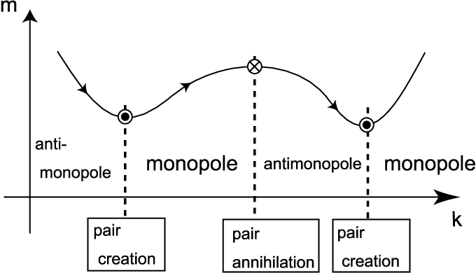
We now return to the present case of the transition between the QSH and the insulator phases. Recall that the string is confined in a restricted region in the direction. Therefore the “string” becomes a “loop”. Then it follows that at the “string” changes its direction in the space, which appears as a pair creation of monopole and antimonopole. Similarly at a pair annihilation of monopole and antimonopole results.
In the particular cases with time-reversal invariance, as we are interested in, the pair creation and pair annihilation appears symmetrically with respect to . Therefore, we expect that the number of loops should be one in the simplest case will be as shown in Fig. 3, and it is indeed realized in the Fu-Kane-Mele model with the term.
Appendix B Calculation of the gapless phase in the Fu-Kane-Mele model with staggered on-site potential
The Hamiltonian matrix for the the Fu-Kane-Mele model with staggered on-site potential is written as
| (36) |
where are the Pauli matrices, and is the 2 2 identity matrix. The coefficients are given by
| (37) | ||||
| (38) |
and , are given similarly to after cyclic permutation of the subscripts , and . We write for brevity. We study when and how the gap closes as the parameters change. Because the gap is between the second and the third bands, we need a condition when the second and third bands have identical eigenenergies. As the codimension is three in this case, the condition should be expressed as three equations, determining a string in space. First we note that the spectrum of is symmetric with respect to , as follows from
| (39) |
where the superscript t denotes matrix transposition, and the unitary matrix is given by
| (40) |
Thus the gap closes if and only if one of the eigenvalues of vanishes, namely, . This renders to
| (41) |
namely,
| (42) |
For given model parameters , , the coupled equations (42) gives gapless points in -space, if any. Such gapless points are stable against small changes of parameters, as we can see as follows. For brevity, let us write the three conditions in Eq. (42) as (, where denotes the set of model parameters. Let be the wavenumber of one of the gapless points. When the model parameters are changed, the values of change accordingly: . The gapless points are then expected to move (). Because the gapless conditions are expanded as
| (43) |
there always exists satisfying these three coupled linear equations. Thus a perturbative change in system parameters moves the gapless points in -space, without removing them.
References
- [1] S. Murakami, N. Nagaosa, and S.-C. Zhang, Science 301, 1348 (2003).
- [2] J. Sinova, D. Culcer, Q. Niu, N. A. Sinitsyn, T. Jungwirth, and A. H. MacDonald, Phys. Rev. Lett. 92, 126603 (2004).
- [3] S. Murakami, N. Nagaosa, and S.-C. Zhang, Phys. Rev. Lett. 93, 156804 (2004).
- [4] C. L. Kane and E. J. Mele, Phys. Rev. Lett. 95, 146802 (2005).
- [5] C. L. Kane and E. J. Mele, Phys. Rev. Lett. 95, 226801 (2005).
- [6] B. A. Bernevig and S.-C. Zhang, Phys. Rev. Lett. 96, 106802 (2006).
- [7] C. Wu, B. A. Bernevig, and S.-C. Zhang, Phys. Rev. Lett. 96, 106401 (2006).
- [8] C. Xu and J. E. Moore, Phys. Rev. B73, 045322 (2006).
- [9] S. Murakami, Phys. Rev. Lett. 97, 236805 (2006).
- [10] B. A. Bernevig, T. L. Hughes, S.-C. Zhang, Science 314, 1757 (2006).
- [11] M. König, S. Wiedmann, C. Brüne, A. Roth, H. Buhmann, L. W. Molenkamp, X.-L. Qi, and S.-C. Zhang Science 318 766-770 (2007).
- [12] L. Fu, C. L. Kane, and E. J. Mele, Phys. Rev. Lett. 98, 106803 (2007).
- [13] J. E. Moore and L. Balents, Phys. Rev. B75, 121306(R) (2007).
- [14] D. Hsieh, D. Qian, L. Wray, Y. Xia, Y. S. Hor, R. J. Cava and M. Z. Hasan, Nature 452, 970 (2008).
- [15] L. Fu and C. L. Kane, Phys. Rev. B74, 195312 (2006).
- [16] S. Murakami, S. Iso, Y. Avishai, M. Onoda, and N. Nagaosa, Phys. Rev. B76, 205304 (2007).
- [17] S. Murakami, New J. Phys.9, 356 (2007); (Corrigendum) ibid. 10, 029802 (2008).
- [18] V. J. von Neumann and E. Wigner, Physik. Zeitschr. 30, 467 (1929).
- [19] C. Herring, Phys. Rev. 52, 361; ibid. 52, 365 (1937).
- [20] E. P. Wigner, Ann. Math. 67, 325 (1958).
- [21] F. J. Dyson, J. Math. Phys. 3, 140 (1962).
- [22] M. V. Berry, Proc. Roy. Soc. London Ser A 392, 45 (1984).
- [23] G. E. Volovik, The Universe in a Helium Droplet, (Oxford University Press, Oxford, 2003).
- [24] M. Kohmoto, Ann. Phys. 160, 343 (1985).
- [25] T. T. Wu and C. N. Yang, Phys. Rev. D12, 3845 (1975).
- [26] S. Raghu, X.-L. Qi, C. Honerkamp and S.-C. Zhang, Phys. Rev. Lett. 100, 156401 (2008).
- [27] F. D. M. Haldane, Phys. Rev. Lett. 61, 2015 (1988).
- [28] G. Montambaux and M. Kohmoto, Phys. Rev. B 41, 11417 (1990).
- [29] R. Shindou and S. Murakami, arXiv:0808.1328.
- [30] S. Murakami and N. Nagaosa, Phys. Rev. Lett. 90, 057002 (2003).