The Precision Determination of Invisible-Particle Masses at the LHC
Abstract
We develop techniques to determine the mass scale of invisible particles pair-produced at hadron colliders. We employ the constrained mass variable , which provides an event-by-event lower-bound to the mass scale given a mass difference. We complement this variable with a new variable which provides an additional upper bound to the mass scale, and demonstrate its utility with a realistic case study of a supersymmetry model. These variables together effectively quantify the ‘kink’ in the function which has been proposed as a mass-determination technique for collider-produced dark matter. An important advantage of the method is that it does not rely simply on the position at the endpoint, but it uses the additional information contained in events which lie far from the endpoint. We found the mass by comparing the HERWIG generated distribution to ideal distributions for different masses. We find that for the case studied, with of integrated luminosity (about signal events), the invisible particle’s mass can be measured to a precision of . We conclude that this technique’s precision and accuracy is as good as, if not better than, the best known techniques for invisible-particle mass-determination at hadron colliders.
1 Introduction
If dark matter is produced at a hadron collider, its likely signature will be missing transverse momentum. To help determine the underlying origin of the observed dark-matter, it is important to measure the masses of the new particle states. Mass determination is a key part to identifying the underlying theory which lies beyond the Standard Model. Newly discovered particles could be Kaluza-Klein (KK) states from extra-dimensions, supersymmetric partners of known states, technicolor hadrons, or something else that we have not anticipated. Models predict relationships between parameters: Supersymmetry relates the couplings of current fermions to the couplings of new bosons and the supersymmetric particle masses reflect the origin of supersymmetry breaking; masses of KK states tell us about the size of the extra dimensions. In general, mass determination of new particle states is central to discerning what lies beyond the Standard Model.
If dark-matter particle states are discovered at the LHC, how will the masses of these new particles be measured? Determining the mass of the dark-matter particle (or other states which decay to dark matter) will be difficult because we don’t expect the dark-matter particles to leave tracks or have a displaced vertex, and because we do not know the rest frame of the initial parton collision.
If one has confidence about the specific model and process responsible for the observed events, then the magnitude of the process’s cross-section constrains the mass. If one does not yet know the model, then model-independent techniques will be needed to determine properties of the newly discovered particles such as couplings, spin, phases, mixing angles, and masses. Proposed methods for finding the gluino phase [1] or spin [2], rely on our ability to make model-independent kinematic mass measurements. Thus, model determination needs a suite of model-independent tools to provide initial constraints on the mass.
There has been much recent work in developing model-independent mass determination tools. Edges in invariant mass combinations provide information about mass differences or mass squared differences [3, 4]. If the hadron collider accesses many new states, then we may be able to determine the masses by combining the relationships provided by many different invariant-mass edges of a cascade decay [5, 6, 7, 8]. There is also a series of approaches called Mass Shell Techniques (MST)11 1 The title MST is suggested in Ref. [9]. where one uses an assumption about the topology and on-shell conditions to solve for the unknown masses. One MST variant assumes a long symmetric cascade decay chain and counts which multiplets of masses have solution to the most events [10], another assumes the masses in two events must be equal [11], and another hybrid combines a MST with the information from the many edges in cascade decays [12] 22 2 The variable is a simple example of such a hybrid technique.. There has been extensive work using the so-called ‘stransverse mass’ variable, , to determine the mass difference between parent particle’s and a dark-matter candidate particle’s mass given an assumed mass for the dark-matter candidate (Refs. [13, 14]have more than 45 citations). If the final decay to the lightest state involves a three-body decay33 3 The presence of a -body decay is a sufficient but not necessary condition. Two-body decays can also display kinks [15, 16] provided the decaying particles have sufficiently large transverse boosts. as shown in Fig. 1, then a ‘kink’ in the [13, 14], will occur at a position which indicates the invisible particle mass, as described by Cho, Choi Kim, Park (CCKP) [17, 18] and corroborated in Refs. [16, 19]. The ‘kink’ in can be quantified by the constrained mass variable that we introduced in a previous letter [20]. Even in models where new invisible particles are nearly massless (like the gravitino studied in [21]), one would rather not just assume the mass of the lightest supersymmetric particle (LSP), which is needed as an input to the traditional analysis, without measuring it in some model independent way. Which approach turns out to be best is likely to depend on what scenario nature hands us, since the various techniques involve different assumptions. Having different approaches also offers the advantage of providing a system of redundant checks.
In Ref. [20], we introduced the kinematic variable which gives an event-by-event lower bound on the dark-matter particle’s absolute mass given the mass difference between the dark matter candidate and its parent. In this paper, we introduce a complementary variable which gives an event-by-event upper bound on the same absolute mass. Our study shows that this technique rivals other invisible-particle mass determination techniques in precision and accuracy.
In this paper, we provides a demonstration of the use of the variable and in LHC conditions. The variables and give an event-by-event lower-bound and upper-bound respectively on the mass of assuming the topology in Fig. 1 and the mass difference . To get the mass difference, we use events where decays into and two visible states via a three-body decay in which we can easily determine the mass difference from the end point of the visible-states invariant-mass distribution, . One might also conceive of a situation with supplementing an alternative technique that gives a tight constraint on the mass difference but may have multiple solutions or a weaker constraint on the mass scale [6][22]. Given this mass difference and enough statistics, ’s endpoint gives the mass of . However the main advantage of the method is that it does not rely simply on the position at the endpoint but it uses the additional information contained in events which lie far from the endpoint. As a result it gives a mass determination using significantly fewer events and is less sensitive to energy resolution and other errors.
To illustrate the method, in this paper we study in detail the performance of the constrained mass variable in a specific supersymmetric model. We study events where each of the two branches have decay chains that end with a decaying to a and a pair of opposite-sign same-flavor(OSSF) leptons. Thus the final states of interest contain four isolated leptons (made up of two OSSF pairs) and missing transverse momentum. Fig 1 defines the four momentum of the particle states with , , and the OSSF pairs forming the visible particles . Any decay products early in the decay chains of either branch are grouped into which we generically refer to as upstream transverse momentum (UTM). Nonzero could be the result of initial state radiation (ISR) or decays of heavier particles further up the decay chain. Events with four leptons and missing transverse momentum have a very small Standard-Model background. To give a detailed illustration of the methods, we have chosen to analyze the benchmark point P1 from [23] which corresponds to mSUGRA with GeV, GeV, , , . Our SUSY particle spectrum was calculated with ISAJET [24] version 7.63. We stress that the analysis technique employed applies generically to models involving decays to a massive particle state that leaves the detector unnoticed.
A powerful feature of the distribution is that, with some mild assumptions, the shape away from the endpoint can be entirely determined from the unknown mass scale and quantities that are measured. The ideal shape fit against early data therefore provides an early mass estimate for the invisible particle. This study is meant to be a guide on how to overcome difficulties in establishing and fitting the shape: difficulties from combinatoric issues, from differing energy resolutions for the leptons, hadrons, and missing transverse momentum, from backgrounds, and from large upstream transverse momentum (UTM) 44 4 Our references to UTM correspond to the Significant Transverse Momentum (SPT), pair production category in [16] where SPT indicates that the relevant pair of parent particles can be seen as recoiling against a significant transverse momentum.. As we shall discuss, UTM actually provides surprising benefits.
The paper is structured as follows: In Section 2, we review and introduce the new observation that, in addition to an event-by-event lower bound on , large recoil against UTM enables one also to obtain an event-by-event upper bound on . We call this quantity . Section 3 describes the modeling and simulation employed. Section 4 discusses the implications of several effects on the shape of the distribution including the (in our case ) distribution, the UTM distribution, the backgrounds, combinatorics, energy resolution, and missing transverse momentum cuts. In Section 5, we put these factors together and estimate the performance. We conclude in Section 6 with a discussion about the performance in comparison to previous work.
2 Upper Bounds on from Recoil against Upstream Transverse Momentum
We will now review the definition of as providing an event-by-event lower bound on . In generalizing this framework, we find a new result that one can also obtain an upper bound on the mass when the two parent particles recoil against some large upstream transverse momentum .
2.1 Review of the Lower Bound on
Fig 1 gives the relevant topology and the momentum assignments. The visible particles and and invisible particle are labeled with with momentum and (which we group into ) and , respectively and in the other branch. We assume that the parent particle is the same in both branches so . Any earlier decay products of either branch are grouped into the upstream transverse momentum (UTM) 4-vector momentum, .

In previous work with events of this topology, we [20] showed how to find an event-by-event lower bound on the true mass of and . We assume that the mass difference can be accurately measured from the invariant mass edges or . For each event, the variable is the minimum value of the mass of (the second lightest state) after minimizing over the unknown division of the missing transverse momentum between the two dark-matter particles :
| (1) | |||||
| (2) | |||||
| (3) | |||||
| (4) | |||||
| (5) |
There are eight unknowns corresponding to the four momentum components of and and five equations of constraint. Because the true and must be within the domain over which we are minimizing, the function is guaranteed to be less than or equal to .
One way of calculating for an event is to use [13, 14, 20], which provides a lower bound on the mass of for an assumed mass of . The true mass of lies along the line where we use to denote the possible masses of and to distinguish it from the true mass of denoted with . Thus we can see that for to be compatible with an event, we must have .
For a given event, if one assumes a mass for , and if the inequality is satisfied, then there is no contradiction, and the event is compatible with this value of . If however, , then we have a contradiction, and the event excludes this value as a viable mass of . Using this observation, can be found for each event by seeking an intersection between and [20]. The lower bound on is given by where is a zero of
| (6) |
In the case , the extreme events analyzed in CCKP [17] demonstrate that will only have one positive zero or no positive zeros, and the slope at a zero will always be negative. For no positive zeros, the lower bound is the trivial lower bound given by . Note that a lower bound on the value of corresponds to a lower bound on the value of . The Appendix in Ref. [20] shows that at the zeros of which satisfy Eq(6), the momenta satisfy Eqns(2-5).
2.2 A New Upper Bound on
If there is large upstream transverse momentum (UTM) () against which the system recoils, then we find a new result. Using the method to calculate gives one the immediate ability to see that can also have an upper bound when requiring Eqns(2-5). This follows because for large UTM the function may have two zeros55 5 There may be regions in parameter space where function has more than two zeros, but we have not encountered such cases in our simulations. which provides both an upper and a lower bound for from a single event. We have also found regions of parameter space where has a single zero but corresponding to an upper bound on the true mass of ( and ) and only the trivial lower bound of .
We can can obtain some insight into the cases in which events with large UTM provides upper bounds on the mass by studying a class of extreme event with two hard jets, and against which recoils (). We will describe this extreme event and solve for the regions of parameter space for which one can analytically see the intersection points giving a lower bound and/or an upper bound. The event is extremal in that , which gives a lower bound on , actually gives the true value of when one selects equal to the true mass .
The ideal event we consider is where a heavier state is pair-produced on shell at threshold. For simplicity we assume the lab-frame is the collision frame. Assume that the s, initially at rest, decay into visible massless jets , and the two states with the decay product momenta and . Both jets have their momenta in the same transverse plane along the negative -axis, and both ’s momentum are directed along the -axis. Finally, in the rest frame of the two s, both decay such that the decay products visible states have their momentum and along the -axis and both invisible massive states have their two momenta along the negative -axis. In the lab frame, the four-vectors are given by
| (7) | |||||
| (8) | |||||
| (9) |
For the event given by Eqns(7-9), we can exactly calculate :
| (10) |
This is found by calculating the transverse mass for each branch while assuming to be the mass of . The value of is chosen so that the transverse masses of the two branches are equal. Substituting this value back into the transverse mass of either branch gives .
Fig 2 shows , given in Eq(6), for several choices of for the process described by Eqs(7-9) with and . Because is the parent of , we must have . If , then is larger than up until their point of intersection at . In this case their point of intersection provides a lower bound as illustrated by the dotted line in Fig. 2 for the case with . For there are two solutions
| (11) | |||||
| (12) |
When , the function has only one zero with the lower bound equalling the upper bound at . The solid line in Fig. 2 shows this case. Between we again have two solutions but this time with
| (13) | |||||
| (14) |
The dashed line in Fig. 2 shows this case with . For greater than this, we have and .

This example illustrates how can provide both a lower-bound and an upper-bound on the true mass for those events with large UTM. The upper-bound distribution provides extra information that can also be used to improve early mass determination, and in what follows we will refer to the upper bound as . We now move on to discuss modeling and simulation of this new observation.
3 Modeling and Simulation
As a specific example of the application of the method, we have chosen a supersymmetry model mSUGRA, GeV, GeV, , , 66 6 This was model from [23] which we also used in [20].. The spectrum used in the simulation has and . We have employed two simulation packages. One is a Mathematica code that creates the ‘ideal’ distributions based only on very simple assumptions and input data. The second is HERWIG [25, 26, 27] which simulates events based on a SUSY spectrum, MSSM cross sections, decay chains, and appropriate parton distribution functions. If the simple Mathematica simulator predicts ‘ideal’ shapes that agree with HERWIG generator, then one has reason to believe that the all the relevant factors relating to the shape are identified in the simple Mathematica simulation. This is an important check in validating the benefits of fitting the and distribution shape as a method to measure the mass of new invisible particles produced at hadron colliders.
3.1 Generation of “Ideal” Distributions
Our ‘ideal’ distributions are produced from a home-grown Monte Carlo event generator written in Mathematica. This generater serves to ensure that we understand the origin of the distribution shape. It also ensures that we have control over measuring the parameters needed to determine the mass without knowing the full model, coupling coefficients, or parton distribution functions. We also use this simulation to determine on what properties the ideal distributions depends.
The simulator is used to create events satisfying the topology shown in Fig 1 for a set of specified masses. We take as given the previously measured mass difference , which we use in all our simulations. We neglect finite widths of the particle states as most are in the sub GeV range for the model we are considering. We neglect spin correlations between the two branches. We perform the simulations in the center-of-mass frame because and are transverse observables and are invariant under longitudinal boosts. The collision energy is distributed according to normalized distribution
| (15) |
unless otherwise specified. The is produced with a uniform angular distribution, and all subsequent decays have uniform angular distribution in the rest frame of the parent. The UTM is simulated by making equal to the UTM with (unless otherwise specified), and boosting the other four-vectors of the event such that the total transverse momentum is zero. As we will show, these simple assumptions capture the important elements of the process. Being relatively model independent, they provide a means of determining the mass for various production mechanisms. If one were to assume detailed knowledge of the production process, it would possible to obtain a better mass determination by using a more complete simulation like HERWIG to provide the ‘ideal’ distributions against which one compares with the data. Here we concentrate on the more model independent simulation to demonstrate that it predicts the and distributions well-enough to perform the mass determination that we demonstrate in this case-study.
3.2 HERWIG “Data”


In order to obtain a more realistic estimate of the problems associated with collision data, we generate samples of unweighted inclusive supersymmetric particle pair production, using the HERWIG Monte Carlo program with LHC beam conditions. These samples produce a more realistic simulation of the event structure that would be obtained for the supersymmetric model studied here, including the (leading order) cross sections and parton distributions. It includes all supersymmetric processes and so contain the relevant background processes as well as the particular decay chain that we wish to study.
Charged leptons ( and ) produced in the decay of heavy objects (SUSY particles and and bosons) were selected for futher study provided they satisfied basic selection criteria on transverse momentum ( GeV) and pseudorapdity (). Leptons coming from hadron decays are usually contained within hadronic jets and so can be experimentally rejected with high efficiency using energy or track isolation criteria. This latter category of leptons was therefore not used in this study. The acceptance criterion used for the hadronic final state was . The detector energy resolution functions used are described in Section 4.2.
4 Factors for Successful Shape Fitting
There are several factors that control or affect the shape of the and distributions. We divide the factors into those that affect the in-principle distribution and the factors that affect the observation of the distribution by the detector like energy resolution and selection cuts.
The in-principle distribution of these events is influenced by the presence or absence of spin-correlations between the branches, the the distribution of the visible particles, any significant upstream transverse momentum (UTM) against which the system is recoiling (e.g. gluinos or squarks decaying further up the decay chain), and background coming from other new-physics processes or the Standard Model. As all these processes effectively occur at the interaction vertex, there are some combinatoric ambiguities. These are the factors that influence the in-principle distribution of events that impinges on the particle detector.
The actual distribution recorded by the detector will depend on further factors. Some factors we are able to regulate – for example cuts on the missing transverse momentum. Other factors depend on how well we understand the detector’s operation – such as the energy resolution and particle identification.
Where the effect of such factors is significant, for example for the , , and background distributions, our approach has been to model their effect on the ideal distributions by using appropriate information from the ‘data’, much as one would do in a real LHC experiment. For the present our ‘data’ are provided by HERWIG, rather than LHC events, but the principle is the same.
4.1 Factors Affecting the In-principle Distribution
- •
Mass Difference and Mass Scale
The end-point of and distributions give the mass of . Therefore the mass scale, , is a dominant factor in the shape of the ‘ideal’ distribution. This is the reason we can use these distributions to determine the mass scale. Fig 4 shows the and distributions for five choices of assuming the HERWIG generated and UTM distributions.

How does the shape change with mass scale? The shape is typically sharply peaked at followed by a tail that ends at the mass of . The peak at is due to events that are compatible with . We say these events give the trivial constraint. Because we bin the data, the height of the first bin depends on the bin size. As becomes larger, then the non-trivial events are distributed over a wider range and the endpoint becomes less clear. In general if all other things are equal, the larger the mass, the more events in the first bin and a longer flatter tail.
The distribution also depends on the mass difference which we assume has been determined. We expect that experimentally one should be able to read off the mass difference from the kinematic end-point with very high precision. Gjelsten, Miller, and Osland estimate this edge can be measured to better than [6, 8] using many different channels that lead to the same edge, and after modeling energy resolution and background.
Errors in the mass determination propagated from the error in the mass difference in the limit of are given approximately by
| (16) |
where is the error in the determination of the mass difference . An error in will lead to an distribution with a shape and endpoint above or below the true mass in the direction indicated by Eq(16).
To isolate this source of error from the uncertainty in the fit, we assume that the mass difference is known exactly in our stated results. In our case an uncertainty of would lead to an additional to be added in quadrature to the error from fitting.
- •
Spin Correlations
There are no spin correlation effects relevant to if the pairs are directly produced and the three-body decay is dominated by the boson (e.g the sleptons are much heavier that ) [20]. There are also no spin correlations if the parents are part of a longer decay chain which involves a scalar at some stage. In the model we are studying, there are enough vertices between the two decays that any correlation is very likely washed out, and we can treat their decays as uncorrelated. In the simple Mathematica simulations, we have assumed no spin dependence in the production of the hypothetical ideal distribution.
- •
Input Distributions
The distribution affects the distribution. Fig 5 shows two distributions and the corresponding distributions with (no UTM). The solid lines show the case where the three-body decay from to is completely dominated by a boson. The dashed line shows the case where the distribution is extracted from the ‘realistic’ HERWIG simulation. We can see that the distribution is affected most strongly in the first several non-zero bins. If we were to determine the mass only from the shape of these first several bins using only the contribution for the difference, we would estimate of the mass to be about GeV below the true mass. This can be understood because the the shape change of the distribution effectively took events out of the first bin and spread them over the larger bins simulating the effect of a smaller mass.


- •
Input Upstream Transverse Momentum Distribution
As we discussed in Section 2, if there is a large upstream transverse momentum (UTM) against which the two ’s recoil, then we have both an upper and lower bound on the mass scale. The left frame of Fig. 6 shows the UTM distribution observed in the ‘realistic’ HERWIG data. The right frame of Fig. 6 shows the and distributions for fixed UTM () of , , , , , and all with . As we discuss under the next bullet, we also find the distribution is not sensitive to the value of . For , these curves begin to approach a common shape. These are ideal upper and lower bound distributions where and . Notice that there is no upper-bound curve for the case with zero UTM. The UTM makes the distribution have a sharper endpoint and thereby make the mass easier to determine. This is equivalent to having a sharper kink in in the presence of large UTM [16].
How do we determine from the data? Because we demand exactly four leptons (two OSSF pairs), we assume all other activity, basically the hadronic activity, in the detector is UTM. The shape used in the ‘ideal’ distribution is a superposition of the different fixed UTM distributions, shown on right frame of Fig. 6, weighted by the observed UTM distribution, shown on the left frame of Fig. 6. Equivalently, we obtain the ideal distribution by selecting in the Mathematica Monte Carlo according to the observed UTM distribution.


- •
Shape Largely Independent of Parton Distributions and Collision Energy
In the limit where there is no UTM, then is invariant under back-to-back boosts of the parent particles; therefore, is also invariant to changes in the parton distribution functions.
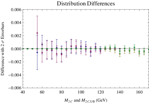
How much of this invariance survives in the presence of large UTM? The answer is that it remains largely independent of the parton collision energy and largely independent of the mass as shown in Fig 7 numerically. On the left frame, we show three distributions and in the right frame their difference with error bars calculated from events. The first distribution assumes , , distributed via 15. The second distribution assumes , , distributed via Eq(15). The third distribution assumes , , and a fixed collision energy of .

- •
Backgrounds

Backgrounds affect the shape and, if not corrected for, could provide a systematic error in the estimated mass. In Section 5 we will see that the position of the minimum in a fit to is barely affected by the background. The main effect of the background is to shift the parabola up, giving a worse fit. To improve the fit, we may be able to estimate the and distribution and magnitude of the background from the data itself. We first discuss the sources of background, and then we describe a generic technique using a Dalitz-like wedgebox analysis to estimate a background model which gives approximately the correct shape and magnitude of the background.
One reason we study the four-lepton with missing transverse momentum channel is because of the very-low Standard-Model background [28, 29]. A previous study [29] estimates about Standard-Model four-lepton events (two OSSF pairs) for with a GeV cut. They suggest that we can further reduce the Standard-Model background by requiring several hadronic jets. Because we expect very-little direct pair production, this would have very little effect on the number of signal events. Also, because s are a part of the intermediate states of these background processes, very few of these events will have significantly different from .
What is the source of these Standard-Model backgrounds? About is from -pair production events with no invisible decay products, in which the missing transverse momentum can only arise from experimental particle identification and resolution errors. This implies that a slightly stronger cut could further eliminate this background. Another are due to production. Not explicitly discussed in their study but representing another possible souce of backgrounds are events containing heavy baryons which decay leptonically. If we assume -quark hadrons decay to isolated leptons with a branching ratio of , then LHC production will lead to about events passing these cuts for where both OSSF leptons pairs have .
Tau decays also provide a background for our specific process of interest. The process will be misidentified as or about of the time. Because the decays introduce new sources of missing transverse momentum (), these events will distort the calculation. This suggests that the dominant background to the hadrons will be from other SUSY processes.
We now create a crude background model from which we estimate the magnitude and distribution of the background using the ‘true’ HERWIG data as a guide. We follow the suggestion of Ref. [9, 29] and use a wedgebox analysis plotting the invariant mass against to supplement our knowledge of the background events mixed in with our signal events. This wedgebox analysis, seen in Fig. 8 for our HERWIG simulation, shows patterns that tell about other SUSY states present. The presence of the strips along GeV indicate that particle states are being created that decay to two leptons via an on-shell . The observation that the intensity changes above and below GeV shows that many of the states produced have one branch that decays via a and the other branch decays via an on-shell . The lack of events immediately above and to the right of the coordinate but below and to the left of coordinate suggest that symmetric process are not responsible for this background.
We also see the density of events in the block above and to the right of suggest a cascade decay with an endpoint near enough to that it is not distinguishable from . Following this line of thinking, we model the background with a guess of an asymmetric set of events where one branch has new states , and with masses such that the endpoint is
| (17) |
and the other branch is our decay. The masses one chooses to satisfy this edge did not prove important so long as the mass differences were reasonably sized; we tried several different mass triplets ending with the LSP, and all gave similar answers.
We now describe the background model used in our fits. One branch starts with a massive state with which decays to a lepton and a new state which in-turn decays to to a lepton and the LSP. The second branch has our signal decay with the decaying to and two leptons via a three-body decay. We added UTM consistent with that observed in the events.
By matching the number of events seen outside the region, we estimate the number of the events within the signal cuts that are due to backgrounds. We estimate of the events with both OSSF pairs satisfying are background events. The model also gives a reasonable distribution for these events. Inspecting the actual HERWIG results showed that actual fraction of background events was . If we let the fraction be free and minimize the with respect to the background fraction, we found a minimum at .
Our background model is simplistic and does not represent the actual processes, but it does a good job of accounting for the magnitude and the shape of the background mixed into our signal distribution. Most of the HERWIG background events came from and charginos which introduce extra sources of missing transverse momentum. Never the less, the shape fit very accurately and the performance is discussed in Section 5. It is encouraging that our estimate of the background shape and magnitude is relatively insensitive to details of the full spectrum. Even ignoring the background, as we will see in Section 5, still leads to a minimum at the correct mass.
- •
Combinatoric Ambiguities
If we assume that the full cascade effectively occurs at the primary vertex (no displaced vertices), then the combinatoric question is a property of the ideal distribution produced in the collisions. There are no combinatoric issues if the two opposite-sign same-flavor lepton pairs are each different flavors. However if all four leptons are the same flavor, we have found that we can still identify unique branch assignments 90% of the time. The unique identification comes from the observation that both pairs must have an invariant mass less than the value of the edge. In of the events, there is only one combination that satisfies this requirement. This allows one to use of the four lepton events without ambiguity. The first are identified from the two OSSF pairs being of different flavors and of the remaining can be identified by requiring both pairs satisfy on which branch. The events which remain ambiguous have two possible assignments, both of which are included with a weight of in the distribution.
4.2 Factors Affecting Distribution Recorded by the Detector
As just described, the ‘ideal’ in-principle distribution is created from the observed distribution and the observed UTM distribution. We include combinatoric effects from events with four leptons of like flavors. Last, we can estimate the magnitude of background events and their and shape. We now modify the in-principle distribution to simulate the effects of the particle detector to form our final ‘ideal’ distribution that includes all anticipated effects. The two main effects on the and distributions are the energy resolution and the cuts.
- •
Shape Dependence on Energy Resolution
Energy resolution causes the and distributions to be smeared. Here we assume the angular resolution is negligible. For both the Mathematica Monte Carlo model and the HERWIG events we simulate the detector’s energy resolution by scaling the four vectors for electrons, muons, and hadrons by
| (18) | |||||
| (19) | |||||
| (20) |
respectively [30][31]. A more detailed detector simulation is of course possible, but since we do not know the true behavior of any LHC detector until the device begins taking data, a more sophisticated treatment would be of limited value here. In practice the dependence of the ideal distribution shapes on the missing transverse momentum resolution should reflect the actual estimated uncertainty of the missing transverse momentum of the observed events.
Smearing of the distributions decreases the area difference between two normalized distributions, thereby decreasing the precision with which one can determine the mass from a given number of signal events. This expanded uncertainty can be seen in Section 5.
The calculations depend on the mass difference, the four-momenta of the four leptons, and the missing transverse momentum. As the lepton energy resolution is very tight, the missing transverse momentum’s energy resolution is dominated by the hadronic energy resolution. We model the energy resolution of the UTM as a hadronic jet. This significantly increases the uncertainty in the missing transverse momentum because hadrons have about five times the energy resolution error.
In our Mathematica model, we represent the UTM as a single four-vector , but in reality it will be the sum of many four-vectors. Because we apply the energy resolution smearing to , if is small the simple Mathematica model will have a smaller missing energy resolution. However, an events with almost UTM could have a large missing momentum energy resolution if it has a lot of hadronic jets whose transverse momentum mostly cancels. Fig 6 shows that most of the time we have considerable hadronic UTM, so this effect is a minor correction on our results.
- •
Shape Dependence on Missing Transverse Momentum Cuts
A key distinguishing feature of these events is missing transverse momentum. To eliminate the large number of Standard Model events with four-lepton and with no , we will need to cut on this parameter. Fig. 9 shows the HERWIG simulation’s missing transverse momentum versus the . A non-trivial requires substantial . Small of less than about only affects the shape below about . The shape of the therefore will require a higher fidelity model from which to train the shapes. Instead, we just choose to not fit bins with .
All events near the end of distribution require significant , therefore cuts will not affect the part of this distribution which we fit. The number of events with no non-trivial upper-bounds will also be affected by cuts. We only fit the distribution up to about .

5 Estimated Performance


Determining the mass based on the shape of the distribution enables one to use all the events and not just those near the end point. We fit both upper-bound and lower-bound shapes to the data as described in the appendix A. As one expects, fitting the lower-bound shape more tightly constrains the mass from below and fitting the upper-bound shape more tightly constrains the mass from above. Combining the two gives approximately even uncertainty. We calculate ideal distributions assuming at five values , , , , and GeV. We then fit a quadratic interpolation through the points. Our uncertainties are based on the value where increases by from its minimum of this interpolation. This uncertainty estimate agrees with about of the results falling within that range after repeated runs. Our uncertainty estimates do not include the error propagated from the uncertainty in the mass difference (see Eq(16)).
We present results for an early LHC run, about , and for the longest likely LHC run before an upgrade, about . After about , we have events ( about signal and background). After , we have about events (about signal and background). Only events out of are from direct pair production. Most of our signal events follow at the end of different decay chains starting from gluinos or squarks. The upstream decay products produce significant UTM against which the two parent particles recoil.
First for the ideal case. After , using only signal events and no energy resolution, the fits to the predicted shapes give (filled circles in Fig. 10). This mass determination can practically be read off from the endpoints seen in Fig. 3; the endpoint is near and subtracting the mass differences gives . We now explore how well we can do with fewer events and after incorporating the effects listed in Section 4.
How does background affect the fit? If we ignore the existence of background in our sample, and we fit all the events to the signal-only shapes, then we find a poor fit shown as the empty circle curve in Fig. 10. By poor fit, we mean the is substantially larger than the bins being compared ( bins from each the upper-bound and lower-bound distributions). Despite this worse fit, the shape fits still give a very accurate mass estimate: after and after . At this stage, we still assume perfect energy resolution and no missing transverse momentum cut.
Next, if we create a background model as described in Section 4, we are able to improve the fit to nearly per bin; the mass estimate remains about the same, but the uncertainty increases by about . We find a small systematic shift (smaller than the uncertainty) in our mass prediction as we increase the fraction of the shape due to the background model vs the signal model. As we increased our fraction of background, we found the mass estimate was shifted down from at background to when we were at background. The best fit occurs with background; which is very close to the we use from the estimate, but farther from the true background fraction of about . With of data, the systematic errors are all but eliminated with the endpoint dominating the mass estimate. These fits are shown as the triangles with dashed lines and give which after the full run becomes .
Including energy resolution as described in Section 4 shows a large increase in the uncertainty. The dashed-line with empty square markers shows the fit when we include both a background model and the effect of including energy resolution. These fits are shown as the empty squares with dashed lines and give which after the full run becomes .
The final shape factor that we account for are the cuts associated with the missing transverse momentum. After we apply cuts requiring and fit only we have our final result shown by the thick lines with filled squares. This includes all cuts, resolution error, combinatorics and backgrounds. We find with events (signal or background) representing , and after this improves to . The true mass on which the HERWIG simulation is based is , so all the estimates are within about of the true mass.

Fig 11 shows the ideal curve expected if including all effects from energy resolution, background, combinatoric, and cuts. The corresponds to the solid square on the left pane of Fig. 10.
The error in mass determination obtained with limited statistics can be estimated using Poisson statistics. In our studies we find that, as one would expect, increasing the number of events by a factor of four, we bring down our error by about a factor of two. This means that one could expect after about which represents signal events and background events.
6 Discussion and Conclusions
Despite adding some of the complicating effects one would encounter with real data, we have discovered other factors which demonstrate one could obtain an even better precision than we originally reported in Ref. [20]. There, we used only our simple Mathematica model that assumed and neglected most sources of realistic uncertainty. We assumed all the events could be modeled as being direct production without spin-correlations. With these simplifications, we argued the mass could be determined to using signal events.
In this paper, we performed a case study to show that that the relevant and shapes can be successfully determined from the mass difference , the distribution observation, the upstream transverse momentum (UTM) distribution observation. We included and accounted for many realistic effects: we modeled the large energy-resolution error of hadronic jets. We also included the effects of backgrounds, cuts, and combinatorics. Our signal and backgrounds were generated with HERWIG. We discussed how a Dalitz-like plot can estimate the background fraction and shape. Observed inputs were used in a simple model to determine ideal distribution shapes that makes no reference to parton distribution functions, cross sections, or other model-dependent factors that we are not likely to know early in the process.
Despite these extra sources of uncertainty, we found a final mass determination of with about signal events which is still better than the appropriately scaled result from Ref. [20]. The sources of the mass determination improvement are twofold: (1) the prediction and fitting of upper-bound distribution, and (2) the sharper end-point in the presence of large UTM. Under equivalent circumstances, the sharper endpoint is enough to give a factor of improvement in the uncertainty over the direct production case assumed in [20]. Fitting the upper bound tends to improve the determination by an additional factor of . This improvement is then used to fight the large hadronic-jet energy resolution and background uncertainty.
Mass determination using and applies to many other processes. We have focused on cases where the mass difference is given by the end-point of an distribution involving a three-body decay. If there is not a three-body decay, then the mass difference may be found by applying other mass determination techniques like the mass shell techniques (MST) [10, 11, 12] or edges in cascade decays [5, 7, 8] or at different stages in symmetric decay chains [22].
How does our method’s performance compare to previous mass determination methods? Firstly, this technique is more robust than the ‘kink’ because in fitting to the shape of the distribution, it does not rely entirely on identification of the events near kinematic boundary. One can view and as variables that event-by-event quantify the ‘kink’. Other than the ‘kink’ technique, the previous techniques surveyed in the introduction apply to cases where there is no three-body decay from which to measure the mass difference directly. However, each of those techniques still constrains the mass difference with great accuracy. The technique of [5, 6, 7, 8] which uses edges from cascade decays determines the LSP mass to with about 500 thousand events from . The approach of [11] assumes a pair of symmetric decay chains and assumes two events have the same structure. They reach using signal events after , but have a systematic bias that needs modeling to remove. By comparison, adjusting to signal events we achieve without a systematic bias after propagating an error of in the mass difference and with all discussed effects. Uncertainty calculations differ amongst groups, some use repeated trial with new sets of Monte Carlo data, and others use . Without a direct comparison under like circumstance, the optimal method is not clear; but it is clear that fitting the and distributions can determine the mass of invisible particles at least as well, if not better than the other known methods in both accuracy and precision.
In summary, we have developed a mass determination technique, based on the constrained transverse mass, which is able to determine the mass of a dark-matter particle state produced at the LHC in events with large missing transverse momentum. The method, which bounds the mass from below, was supplemented by a new distribution which bounds the mass from above in events with large upstream transverse momentum. A particular advantage of the method is that it also obtains substantial information from events away from the end point allowing for a significant reduction in the error. The shape of the distribution away from the end-point can be determined without detailed knowledge of the underlying model, and as such, can provide an early estimate of the mass. Once the underlying process and model generating the event has been identified the structure away from the end-point can be improved using, for example, HERWIG to produce the process dependent shape. We performed a case-study simulation under LHC conditions to demonstrate that mass-determination by fitting the and distributions survives anticipated complications. With this fitting procedure it is possible to get an early measurement of the mass - with just 400 signal events in our case study we found we would determine . The ultimate accuracy obtainable by this method is . We conclude that this technique’s precision is as good as, if not better than, the best existing techniques.
Acknowledgements
We also want to thank Chris Lester for very helpful conversations and comments on the manuscript, and Laura Serna for reviewing the manuscript. MS acknowledges support from the United States Air Force Institute of Technology. This work was partly supported by the Science and Technology Facilities Council of the United Kingdom. The views expressed in this paper are those of the authors and do not reflect the official policy or position of the United States Air Force, Department of Defense, or the US Government.
Appendix A Appendix A: Least squares fit
In order to determine we perform a fit between ideal distributions and the HERWIG data. First for definitions: We define as the number of events in the region to be fit, and likewise is the number of events in the region to be fit. The of the events are grouped into bins; counts the events in the bin. The variable is the normalized distribution of ideal events expected in bin as calculated with an assumed , the measured , the observed distribution, the observed UTM distribution, and the appropriate detector simulator. We likewise define the upper bound distribution to be . We also define the background distribution for lower-bound and upper-bound distributions to be and and the fraction of the total events we estimate are from background .
Assuming a Poisson distribution, we assign an uncertainty, , to each bin given by
| (21) |
and likewise for the upper-bound distribution. The second term has been added to ensure an appropriate weighting of bins with very few events that does not bias the fit towards or away from this end-point. In bins with few counts, normal Poisson statistics does not apply77 7 By this we mean that has a large percent error when used as a predictor of the number of counts when is less than about 5..
The is given by
| (22) | |||||
We calculate ideal distributions for . We fit quadratic interplant through the points. The minimum of the interplant is our estimate of . The amount changes for an increase in by one gives our uncertainty, , for [32].
References
- [1] S. Mrenna, G. L. Kane, and L.-T. Wang, Measuring gaugino soft phases and the LSP mass at Fermilab, Phys. Lett. B483 (2000) 175–183, [hep-ph/9910477].
- [2] G. L. Kane, A. A. Petrov, J. Shao, and L.-T. Wang, Initial determination of the spins of the gluino and squarks at LHC, 0805.1397.
- [3] B. C. Allanach, C. G. Lester, M. A. Parker, and B. R. Webber, Measuring sparticle masses in non-universal string inspired models at the LHC, JHEP 09 (2000) 004, [hep-ph/0007009].
- [4] B. C. Allanach, J. P. Conlon, and C. G. Lester, Measuring Smuon-Selectron Mass Splitting at the CERN LHC and Patterns of Supersymmetry Breaking, Phys. Rev. D77 (2008) 076006, [0801.3666].
- [5] H. Bachacou, I. Hinchliffe, and F. E. Paige, Measurements of masses in sugra models at lhc, Phys. Rev. D62 (2000) 015009, [hep-ph/9907518].
- [6] B. K. Gjelsten, D. J. Miller, and P. Osland, Measurement of SUSY masses via cascade decays for SPS 1a, JHEP 12 (2004) 003, [hep-ph/0410303].
- [7] C. G. Lester, Constrained invariant mass distributions in cascade decays: The shape of the ’m(qll)-threshold’ and similar distributions, Phys. Lett. B655 (2007) 39–44, [hep-ph/0603171].
- [8] B. K. Gjelsten, D. J. Miller, P. Osland, and A. R. Raklev, Mass determination in cascade decays using shape formulas, AIP Conf. Proc. 903 (2007) 257–260, [hep-ph/0611259].
- [9] M. Bisset, N. Kersting, and R. Lu, Improving SUSY Spectrum Determinations at the LHC with Wedgebox and Hidden Threshold Techniques, 0806.2492.
- [10] H.-C. Cheng, J. F. Gunion, Z. Han, G. Marandella, and B. McElrath, Mass Determination in SUSY-like Events with Missing Energy, JHEP 12 (2007) 076, [0707.0030].
- [11] H.-C. Cheng, D. Engelhardt, J. F. Gunion, Z. Han, and B. McElrath, Accurate Mass Determinations in Decay Chains with Missing Energy, 0802.4290.
- [12] M. M. Nojiri, G. Polesello, and D. R. Tovey, A hybrid method for determining SUSY particle masses at the LHC with fully identified cascade decays, JHEP 05 (2008) 014, [0712.2718].
- [13] C. G. Lester and D. J. Summers, Measuring masses of semi-invisibly decaying particles pair produced at hadron colliders, Phys. Lett. B463 (1999) 99–103, [hep-ph/9906349].
- [14] A. Barr, C. Lester, and P. Stephens, m(T2): The truth behind the glamour, J. Phys. G29 (2003) 2343–2363, [hep-ph/0304226].
- [15] B. Gripaios, Transverse observables and mass determination at hadron colliders, arXiv:0709.2740 [hep-ph].
- [16] A. J. Barr, B. Gripaios, and C. G. Lester, Weighing Wimps with Kinks at Colliders: Invisible Particle Mass Measurements from Endpoints, JHEP 02 (2008) 014, [0711.4008].
- [17] W. S. Cho, K. Choi, Y. G. Kim, and C. B. Park, Gluino Stransverse Mass, Phys. Rev. Lett. 100 (2008) 171801, [0709.0288].
- [18] W. S. Cho, K. Choi, Y. G. Kim, and C. B. Park, Measuring superparticle masses at hadron collider using the transverse mass kink, JHEP 02 (2008) 035, [0711.4526].
- [19] M. M. Nojiri, Y. Shimizu, S. Okada, and K. Kawagoe, Inclusive transverse mass analysis for squark and gluino mass determination, 0802.2412.
- [20] G. G. Ross and M. Serna, Mass Determination of New States at Hadron Colliders, Physics Letters B (2008) [0712.0943]. In-press.
- [21] K. Hamaguchi, E. Nakamura, and S. Shirai, A Measurement of Neutralino Mass at the LHC in Light Gravitino Scenarios, 0805.2502.
- [22] M. Serna, A short comparison between and , JHEP 06 (2008) 004, [0804.3344].
- [23] W. Vandelli, Prospects for the detection of chargino-neutralino direct production with ATLAS detector at the LHC. PhD thesis.
- [24] F. E. Paige, S. D. Protopopescu, H. Baer, and X. Tata, ISAJET 7.69: A Monte Carlo event generator for p p, anti-p p, and e+ e- reactions, hep-ph/0312045.
- [25] G. Corcella et. al., HERWIG 6.5 release note, hep-ph/0210213.
- [26] S. Moretti, K. Odagiri, P. Richardson, M. H. Seymour, and B. R. Webber, Implementation of supersymmetric processes in the HERWIG event generator, JHEP 04 (2002) 028, [hep-ph/0204123].
- [27] G. Marchesini et. al., HERWIG: A Monte Carlo event generator for simulating hadron emission reactions with interfering gluons. Version 5.1 - April 1991, Comput. Phys. Commun. 67 (1992) 465–508.
- [28] D. K. Ghosh, R. M. Godbole, and S. Raychaudhuri, Signals for r-parity-violating supersymmetry at a 500-gev e+ e- collider, hep-ph/9904233.
- [29] M. Bisset, N. Kersting, J. Li, F. Moortgat, and Q. Xie, Pair-produced heavy particle topologies: Mssm neutralino properties at the lhc from gluino / squark cascade decays, Eur. Phys. J. C45 (2006) 477–492, [hep-ph/0501157].
- [30] ATLAS Collaboration, S. Akhmadalev et. al., Hadron energy reconstruction for the ATLAS calorimetry in the framework of the non-parametrical method, Nucl. Instrum. Meth. A480 (2002) 508–523, [hep-ex/0104002].
- [31] A. Collaboration, ATLAS computing : Technical design report, CERN, ATLAS-TDR-017,CERN-LHCC-2005-022 (2005).
- [32] P. Bevington and K. Robinson, Data Reduction and Error Analysis in the Physics Sciences. McGraw Hill, second edition ed., 1992.