Linear Covariant Gauges on the Lattice
Abstract
Linear covariant gauges, such as Feynman gauge, are very useful in perturbative calculations. Their nonperturbative formulation is, however, highly non-trivial. In particular, it is a challenge to define linear covariant gauges on a lattice. We consider a class of gauges in lattice gauge theory that coincides with the perturbative definition of linear covariant gauges in the formal continuum limit. The corresponding gauge-fixing procedure is described and analyzed in detail, with an application to the pure case. In addition, results for the gluon propagator in the two-dimensional case are given.
Keywords:
Lattice gauge theory; Gauge fixing; Covariant gaugesPACS
11.15.Ha , 12.38.Aw , 14.70.Dj1 Introduction
Many direct experimental tests of QCD are performed at large energies. In this regime, the contributions obtainable in perturbation theory are dominant. Such perturbative calculations are often most conveniently done in linear covariant gauges, such as Feynman gauge (see for example [1]). On the other hand, the continuation of these gauges to the non-perturbative regime and, in particular, their definition on the lattice is not trivial. Only for one particular representative of this class of gauges, i.e. the Landau gauge, have non-perturbative studies on the lattice been thoroughly carried out. For this gauge, progress has been made in the understanding of the infrared sector of the theory, in particular through study of correlation functions. This was possible by a combination of various methods, such as Dyson-Schwinger equations [2, 3, 4, 5, 6, 7, 8, 9, 10, 11, 12, 13, 14, 15], renormalization-group methods [11, 16, 17], stochastic quantization [18, 19], lattice calculations [20, 21, 22, 23, 24, 25, 26, 27, 28, 29, 30, 31, 32, 33, 34, 35, 36, 37, 38, 39, 40, 41, 42] and studies [43, 44] based on the Gribov-Zwanziger action [45].
In covariant gauges beyond Landau gauge, only a few results are presently available [46, 47, 48, 49, 50]. Some of these [48, 49] suggest that the Gribov-Zwanziger confinement mechanism [18, 19, 51, 52, 53], proposed for Coulomb and Landau gauge, may also be at work in the complete class of linear covariant gauges. Nevertheless, a full understanding of how non-perturbative effects, and especially confinement, manifest themselves in linear covariant gauges is still lacking.
The aim of this work is to provide a non-perturbative implementation of linear covariant gauges in lattice gauge theory that goes beyond previous attempts [46]. In Section 2 the non-perturbative definition of linear covariant gauges will be discussed. In Section 3 one possible implementation on the lattice will be introduced. The properties of the proposed algorithm will be studied in Section 4, showing that this gauge definition tends to the definition of the ordinary linear covariant gauge in the continuum limit. Finally, as an example, the gluon propagator is presented in Sections 4.2 and 5. We consider the two and three-dimensional cases and the SU(2) gauge group in order to study quantitatively the approach to the continuum. Our results are summarized in Section 6. Technical details for the generation of configurations using the Wilson action and for the Landau gauge fixing can be obtained from Ref. [30]. The sets of configurations (in the 2d case) employed for this work are listed separately for each of the three considered physical volumes in Tables 1-3.
| [fm] | [GeV] | [fm] | Sweeps | Configs | ||
|---|---|---|---|---|---|---|
| 3.55 | 20 | 10 | 1.11 | 0.178 | 30 | 2623 |
| 3.55 | 30 | 21.95 | 1.66 | 0.118 | 40 | 2534 |
| 3.55 | 40 | 38.6 | 2.22 | 0.0888 | 50 | 2927 |
| 3.55 | 50 | 60 | 2.77 | 0.0710 | 60 | 4654 |
| 3.55 | 60 | 86.3 | 3.32 | 0.0592 | 70 | 3563 |
| 3.55 | 70 | 117.4 | 3.88 | 0.0507 | 80 | 4275 |
| 3.55 | 80 | 153 | 4.43 | 0.0444 | 90 | 6107 |
| 3.55 | 90 | 193.7 | 4.99 | 0.0394 | 100 | 8328 |
| 3.55 | 100 | 239 | 5.54 | 0.0355 | 110 | 7195 |
| 3.55 | 120 | 344 | 6.65 | 0.0296 | 130 | 7580 |
| 3.55 | 140 | 468 | 7.76 | 0.0254 | 150 | 5227 |
| 3.55 | 160 | 611 | 8.86 | 0.0222 | 170 | 2982 |
| 3.55 | 180 | 773 | 9.97 | 0.0197 | 190 | 2204 |
| 3.55 | 200 | 954 | 11.1 | 0.0178 | 210 | 1032 |
| 3.55 | 220 | 1155 | 12.2 | 0.0162 | 230 | 959 |
| 3.55 | 242 | 1397 | 13.4 | 0.0147 | 252 | 587 |
| 3.55 | 266 | 1689 | 14.8 | 0.0133 | 276 | 210 |
| 3.55 | 294 | 2062 | 16.3 | 0.0121 | 304 | 166 |
| 3.55 | 324 | 2505 | 18.0 | 0.0110 | 334 | 87 |
| [fm] | [GeV] | [fm] | Sweeps | Configs | ||
| 7.11 | 40 | 10 | 1.11 | 0.178 | 50 | 2633 |
| 7.11 | 50 | 15.35 | 1.39 | 0.142 | 60 | 2916 |
| 7.11 | 60 | 21.9 | 1.66 | 0.119 | 70 | 3973 |
| 7.11 | 70 | 29.63 | 1.94 | 0.102 | 80 | 4263 |
| 7.11 | 80 | 38.55 | 2.22 | 0.0889 | 90 | 4466 |
| 7.11 | 90 | 48.65 | 2.49 | 0.0790 | 100 | 6507 |
| 7.11 | 100 | 59.9 | 2.77 | 0.0711 | 110 | 6534 |
| 7.11 | 120 | 86.1 | 3.32 | 0.0593 | 130 | 6785 |
| 7.11 | 140 | 117 | 3.88 | 0.0508 | 150 | 5874 |
| 7.11 | 160 | 152.7 | 4.43 | 0.0444 | 170 | 3950 |
| 7.11 | 180 | 193 | 4.99 | 0.0395 | 190 | 1744 |
| 7.11 | 200 | 238.4 | 5.54 | 0.0356 | 210 | 1391 |
| 7.11 | 220 | 288 | 6.09 | 0.0323 | 230 | 605 |
| 7.11 | 242 | 349 | 6.72 | 0.0294 | 252 | 457 |
| 7.11 | 266 | 421 | 7.38 | 0.0267 | 276 | 374 |
| 7.11 | 294 | 514.6 | 8.09 | 0.0242 | 304 | 134 |
| 7.11 | 324 | 625 | 8.99 | 0.0219 | 334 | 80 |
| [fm] | [GeV] | [fm] | Sweeps | Configs | ||
| 14.2 | 80 | 10 | 1.11 | 0.178 | 90 | 4111 |
| 14.2 | 90 | 12.55 | 1.25 | 0.158 | 100 | 4736 |
| 14.2 | 100 | 15.4 | 1.39 | 0.142 | 110 | 5455 |
| 14.2 | 120 | 21.9 | 1.66 | 0.118 | 130 | 6724 |
| 14.2 | 140 | 29.7 | 1.94 | 0.101 | 150 | 6245 |
| 14.2 | 160 | 38.6 | 2.22 | 0.0888 | 170 | 4372 |
| 14.2 | 180 | 48.8 | 2.49 | 0.0789 | 190 | 2108 |
| 14.2 | 200 | 60.1 | 2.77 | 0.0710 | 210 | 1533 |
| 14.2 | 220 | 72.6 | 3.05 | 0.0647 | 230 | 582 |
| 14.2 | 242 | 87.8 | 3.35 | 0.0588 | 252 | 596 |
| 14.2 | 266 | 103 | 3.69 | 0.0534 | 276 | 465 |
| 14.2 | 294 | 129.4 | 4.08 | 0.0483 | 304 | 119 |
| 14.2 | 324 | 157 | 4.50 | 0.0438 | 334 | 107 |
2 Non-perturbative definition of linear covariant gauges
Linear covariant gauges are defined by the average over gauge configurations satisfying
| (1) |
for arbitrary real-valued functions . [Here is the gluon field and is the color index, taking values for the SU() gauge group.] This average is usually done by considering the partition function
| (2) |
i.e. by using a Gaussian average of width with the gauge-fixing parameter . (Note that, with the usual convention , this gauge-fixing parameter is dimensionless for any space-time dimension .) At the same time, the mean of the distribution is the (in perturbation theory unique) Landau-gauge configuration
| (3) |
Thus, in perturbation theory, the linear covariant gauge is an average over the complete gauge orbit [as can take any value], with Gaussian weight around the Landau gauge.
The problem to be solved is to introduce a non-perturbative gauge prescription and to discretize it on a lattice. Of course, at the non-perturbative level, effects due to Gribov copies may be difficult to single out and to quantify. Nevertheless, in the lattice gauge-fixing procedure introduced in the next section, the determined gauge copy is actually unique, up to ambiguities involved in defining the (minimal) Landau gauge and to (possible) numerical artifacts.
Let us note that previous attempts to formulate this class of linear covariant gauges [46] relied on the absence of (non-trivial) zero-modes of the Faddeev-Popov operator on the lattice in the Landau gauge. On the other hand we know that, in the infinite-volume limit, Landau-gauge configurations belong to the so-called first Gribov horizon [30, 34, 55, 56], i.e. such zero-modes do exist. Thus, it is not clear whether the procedure described in [46] is well defined. Moreover, in that case one obtains on the lattice a Faddeev-Popov operator which is different from the corresponding continuum operator. Here we use a different approach, which is not based on the above assumption. This gauge-fixing procedure is described in the following section and it will be called a quasi-linear covariant gauge.
3 Quasi-linear covariant gauges on the lattice
Our gauge-fixing prescription is a very direct implementation of the prescription for performing a Gaussian average around the Landau gauge.
The first step is to transform a given (thermalized) gauge-field configuration to Landau gauge (see for example [57, 58, 59, 60]). Note that, in principle, in this step it is necessary to fix the Landau gauge completely, i.e. to select a configuration within the fundamental modular region [52, 61], corresponding to the absolute minimum of the minimizing functional. However, the practical implementation of this step is still an open problem [27, 37]. On the other hand, it has been conjectured [62] that, if one determines only correlation functions of a finite number of field operators, it is sufficient to fix the gauge to a copy inside the first Gribov region, i.e. these Gribov copies should be equivalent for very large volumes. Hence, in our quasi-linear covariant gauge, the Landau gauge configuration is chosen inside the first Gribov region.
The second step is to obtain a configuration that satisfies Eq. (1), for a given , starting from the configuration fixed to Landau gauge (in the first step). This can be obtained by recalling that, for an infinitesimal gauge transformation
| (4) |
the gluon field gets modified to
| (5) |
Here we indicate with the identity matrix, are the generators of the SU() Lie algebra, is the covariant derivative defined as
| (6) |
is the bare coupling constant and are the structure constants of the gauge group. Thus, if one finds as a solution of the equations
| (7) |
then we have
| (8) |
where we used the fact that the original gluon field satisfies the Landau-gauge condition . Of course, this procedure is correct only if the gauge transformation is small. On the other hand, as we will see below, terms that are of higher order in should become smaller in the continuum limit. Let us also note that Eq. (7) above can easily be solved, using for example a Conjugate Gradient iterative method, since the Landau-gauge Faddeev-Popov matrix is semi-positive definite. Of course, for a finite lattice volume , the functions should be orthogonal to the trivial (constant) zero-modes of . Numerically this means that the constant mode has to be explicitly removed from before starting the inversion of . In the infinite-volume limit the functions should also be orthogonal to the non-trivial zero-modes11 1 We did not investigate if the presence of these non-trivial zero-modes hampers the definition of linear covariant gauges for . of .
Furthermore, on the lattice, the gauge transformation is applied to the group-valued link variables and for a given we need to define a group-valued gauge transformation . In the SU(2) case this can easily be done by considering
| (9) | |||||
| (10) |
where are the Pauli matrices and summation over color indices is understood.22 2 This procedure can in principle be extended to any simple Lie group. In particular, the determination of the generators of the gauge transformation , using the prescription (7), is valid for any gauge group. On the other hand, a simple map relating to , such as Eq. (9), is usually not available and one should probably rely on numerical methods in order to obtain the group element . Clearly, in the limit of small one finds the infinitesimal gauge transformation (4), if we identify the Pauli matrices with the generators of the SU(2) Lie algebra. For finite , the algebra-valued fields , obtained from the link variables after this gauge transformation, will thus not satisfy exactly the gauge condition (8). Nevertheless the agreement is correct up to corrections of order , becoming exact in the formal continuum limit. Indeed, besides the usual errors, induced by the definition of the gluon field, Eq. (7) is correct only for the infinitesimal gauge transformation (4). By considering the finite gauge transformation (9), one indroduces errors of order . From Eqs. (5) and (6) one sees that has dimension , i.e. it has mass dimension , where is the space-time dimension. Note that, to be more consistent, one should write the infinitesimal gauge transformation (5) as . Thus, in the continuum limit these errors go indeed to zero. Of course, it would be interesting to study possible improvements for Eq. (7), in order to speed-up the approach to the continuum. This also shows that our approach is not unique and other choices for the gauge transformation are possible, leading to different subleading behaviors.
Finally, in the third step, we need to average over gauge copies satisfying (1). As said above, the quantities are randomly chosen using a Gaussian distribution with null mean value and width . This implies that is unbounded. On the other hand, on the lattice, using a compact formulation, the field is bounded and so is its derivative . Thus, cannot really obey a Gaussian distribution and in general it is not possible to satisfy Eq. (1) on a discrete lattice for an arbitrary function (see Appendix B.2 in [63]). Nevertheless, we can still define a gauge-fixing procedure that becomes a linear covariant gauge in the formal continuum limit. To this end we note that, on the lattice, the Gaussian distribution in Eq. (2) can be written as
| (11) |
Here, the factor is necessary in order to obtain the correct continuum limit. Indeed, working in the continuum in a generic -dimensional space, Eq. (1) can be made dimensionless by multiplying both sides by . By recalling that in dimensions it is clear that the lattice quantity
| (12) |
becomes
| (13) |
in the formal continuum limit. Thus, on the lattice, the function is generated from a Gaussian distribution with width at each site and for each color. Note that in the continuum limit the width of the distribution shrinks to zero. Therefore, the functions depart less from zero and the gauge fixing can be achieved using a small gauge transformation for nearly all gauge copies entering into the average (2). Note that this process is slower for larger , since the width of the Gaussian scales with .


Finally, if one considers the partition function (2) it is clear that, in order to evaluate an observable in the linear covariant gauge, one needs to perform two averages: one is the usual average over configurations , while the other is the one along the gauge orbit . Thus, the space to be sampled is and errors should be estimated by regarding each sample from as an independent configuration. Of course, in order to sample correctly this product space, one needs to generate enough thermalized configurations and, for each configuration, a sufficient number of Gaussian-distributed copies on the given gauge orbit. How large should be clearly depends on the considered observables. For correlation functions such as the gluon propagator we find that, if the number of thermalized configurations is large enough, then a very small number for yields a result that does not change significantly by increasing , as shown in Fig. 1. This implies that the fluctuations along a gauge orbit are smaller than between different orbits.
4 Properties of the gauge-fixing


In this section we study the extrapolation to the continuum limit of the gauge-fixing condition described in the previous section. The results depend, of course, on the value of , i.e. on the width of the Gaussian distribution. Here we consider the case (Feynman gauge) for the calculations in three dimensions. Below, in two dimensions, we will consider the case .
4.1 First moment
Our first check refers to the distributions of the one-point correlation function , where is defined in Eq. (5). Since is generated using a Gaussian distribution, one should in principle obtain that the quantity , evaluated after fixing the configuration to the quasi-linear covariant gauge, should also obey a Gaussian distribution with the same width. On the other hand, due to discretization errors and to the finite-precision arithmetic employed in the determination of , one can expect deviations from the original Gaussian distribution. Thus, this check is a simple and direct way to measure the quality of the gauge fixing and the deviation from the continuum gauge condition (8). Results are reported in Fig. 2 and in Table 4 for three different lattice volumes in 3d with (roughly) the same physical volume (2.1 fm)3. We find that in the three cases the width of the distribution of is in rather good agreement with the original distribution, since the measured value of the gauge-fixing parameter is very close to 1. The deviation from 1 is actually expected, and corresponds to the necessity of renormalizing in linear covariant gauges. We also find that the gauge-fixing procedure does not introduce skewness, while in the three cases a non-vanishing kurtosis is clearly observable. On the other hand, this kurtosis is decreasing with increasing (see Table 4). Also note (see Fig. 2) that the distribution of becomes visibly different from that of for values on the y-axis of about at , at and at .
| Kurtosis | ||||
|---|---|---|---|---|
| 4.2 | 1 | 0.978 | 0.539 | |
| 6.0 | 1 | 0.953 | 0.124 | |
| 9.0 | 1 | 0.951 | 0.00977 |
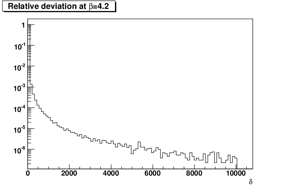
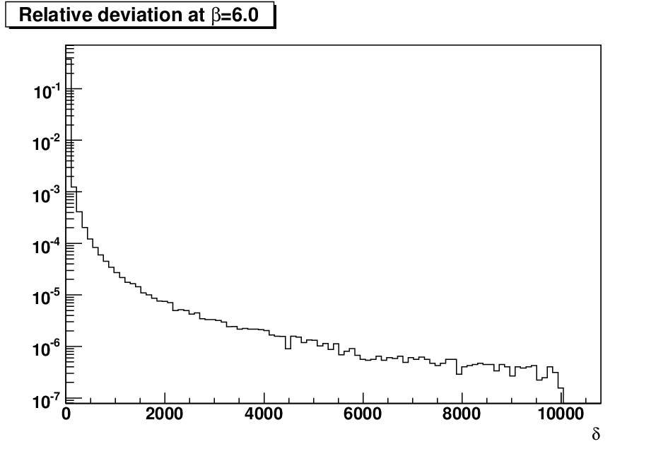
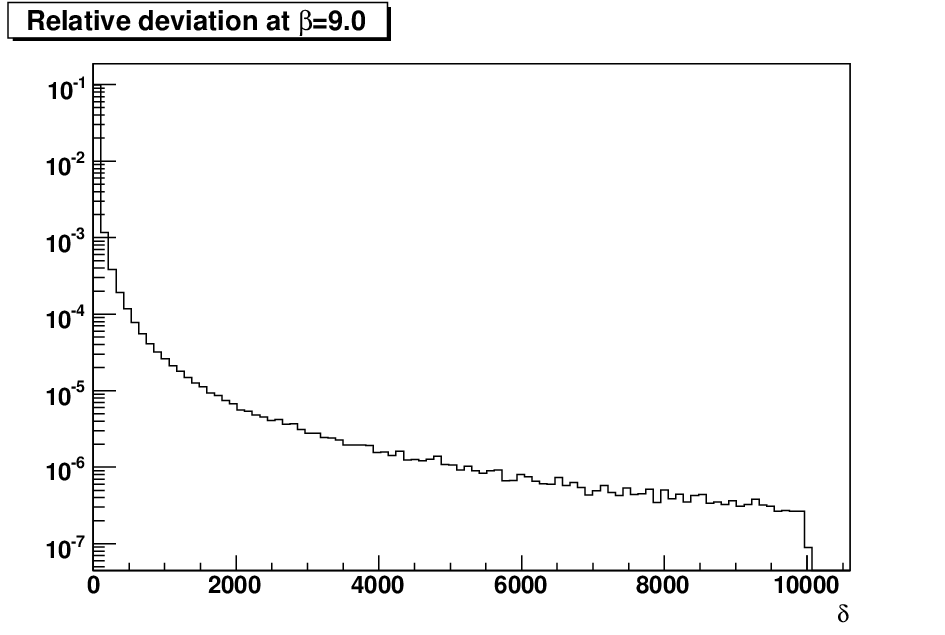
We also evaluated the relative (pointwise) deviation
| (14) |
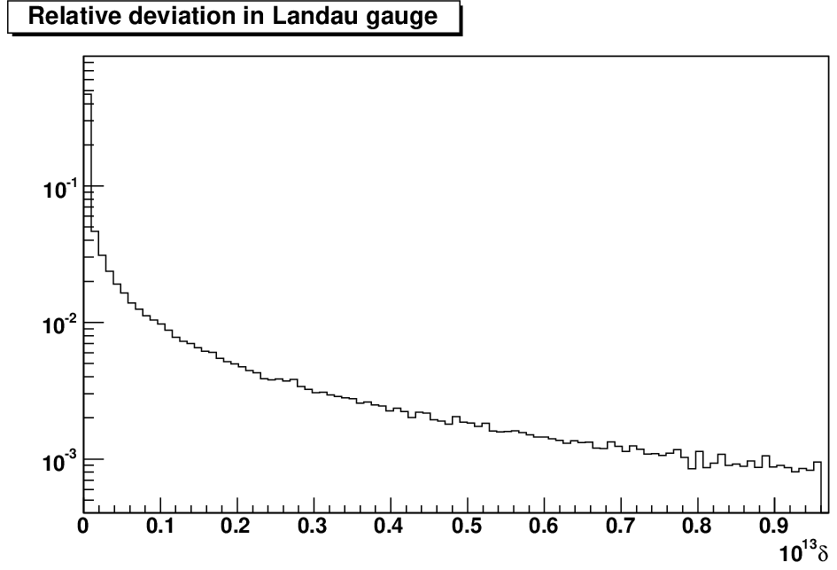
Results are shown in Fig. 3 for the same set of configurations considered in Fig. 2. Clearly we always find sites where is very large. However, the maximal value of as well as the number of sites with large relative deviation, both in absolute number and normalized to the total number of sites, is decreasing with increasing , even though this is not clearly visible from the plots. E. g., at the cutoff value considered in Fig. 3, the value in the y-axis is about , and , respectively at , 6.0 and 9.0. Since the histograms are normalized to a unit area, this implies that the probability of such a large deviation is reduced at large . A possible source for the very large deviations is likely related to functions that exceed the range that can be covered by and using the compact formulation on the lattice.
4.2 Second moment: The longitudinal gluon propagator
We have seen in the above section that, if one considers single-site properties, the quasi-linear covariant gauge indeed seems to approach the usual linear covariant gauge in the limit . On the other hand, we should check if the same is true for all correlation functions of . Here we consider only the two-point correlation functions of , since higher correlation functions are statistically very noisy [30].

In the case of the two-point correlation function
| (16) |
the distribution should be proportional to . By applying the Fourier-transform one finds the well-known Slavnov-Taylor identity (STI) that the longitudinal part of the gluon propagator does not become dressed and is proportional to , with the renormalized gauge parameter appearing in the constant of proportionality [1]
Let us recall that this STI is a trivial consequence of the gauge condition. Thus, its violation as a function of is a useful check in order to control the extrapolation to the continuum limit.
Results for the longitudinal part of the gluon propagator, defined as33 3 Here we did not consider the mid-link Fourier transform of the gluon field [64]. However, the behaviors of the longitudinal gluon propagator for momenta along the -axis and along the -diagonal are rather similar (see Fig. 4), suggesting that discretization effects related to the definition of the gluon field in momentum space are quite small.
| (17) |
are reported in Fig. 4 for the case . This value of was chosen, instead of the Feynman gauge , in order to speed up the approach to the continuum limit. One clearly sees that the dressing function is far from flat, but is becoming slowly flatter with increasing . Only at large momenta does one find an essentially constant function. However, also at large momenta, renormalization effects are clearly visible. They can be quantified by evaluating the renormalization factors using the relation and renormalization condition
| (18) |
Results are reported in Table 5. The increase of with is consistent with a logarithmic evolution, in accordance with the perturbative expectation. Moreover, this evolution depends on the considered physical lattice volume, being faster for larger volumes. As tends to infinity in the limit , the attraction of the Landau gauge as a fixed point is evident.
| [fm] | [fm] | [fm] | |||||||
| 20 | 10 | 3.55 | 1.003(2) | ||||||
| 30 | 21.95 | 3.55 | 1.010(2) | ||||||
| 40 | 38.6 | 3.55 | 1.013(2) | 10 | 7.11 | 1.030(7) | |||
| 50 | 60 | 3.55 | 1.013(1) | 15.35 | 7.11 | 1.00(1) | |||
| 60 | 86.3 | 3.55 | 1.014(3) | 21.9 | 7.11 | 1.031(3) | |||
| 70 | 117.4 | 3.55 | 1.012(2) | 29.63 | 7.11 | 1.045(3) | |||
| 80 | 153 | 3.55 | 1.013(1) | 38.55 | 7.11 | 1.053(2) | 10 | 14.2 | 1.017(8) |
| 90 | 193.7 | 3.55 | 1.011(3) | 48.65 | 7.11 | 1.061(3) | 12.55 | 14.2 | 1.02(1) |
| 100 | 239 | 3.55 | 1.011(1) | 59.9 | 7.11 | 1.064(1) | 15.4 | 14.2 | 1.088(8) |
| 120 | 344 | 3.55 | 1.011(1) | 86.1 | 7.11 | 1.062(3) | 21.9 | 14.2 | 1.203(4) |
| 140 | 468 | 3.55 | 1.014(1) | 117 | 7.11 | 1.064(1) | 29.7 | 14.2 | 1.231(5) |
| 160 | 611 | 3.55 | 1.018(2) | 152.7 | 7.11 | 1.067(2) | 38.6 | 14.2 | 1.248(3) |
| 180 | 773 | 3.55 | 1.018(2) | 193 | 7.11 | 1.073(3) | 48.8 | 14.2 | 1.21(1) |
| 200 | 954 | 3.55 | 1.024(3) | 238.4 | 7.11 | 1.072(3) | 60.1 | 14.2 | 1.272(8) |
| 220 | 1155 | 3.55 | 1.022(3) | 288 | 7.11 | 1.079(4) | 72.6 | 14.2 | 1.277(6) |
| 242 | 1397 | 3.55 | 1.026(4) | 349 | 7.11 | 1.083(9) | 87.8 | 14.2 | 1.294(5) |
| 266 | 1689 | 3.55 | 1.037(7) | 421 | 7.11 | 1.078(6) | 103 | 14.2 | 1.306(6) |
| 294 | 2062 | 3.55 | 1.038(8) | 514.6 | 7.11 | 1.093(9) | 129.4 | 14.2 | 1.31(1) |
| 324 | 2505 | 3.55 | 1.05(1) | 625 | 7.11 | 1.12(1) | 157 | 14.2 | 1.31(3) |
In any case, the main finite- effects can be seen at low momenta. Indeed, there is a clear maximum in the longitudinal gluon dressing function for momenta of about 0.5–1 GeV (see Fig. 4). We also find that this maximum seems to become flatter as increases, even though this appears as a remarkably slow process. In addition, the height of the maximum increases with the physical volume. The dependence of this maximum is shown in Fig. 5. One sees that, for small , the maximum seems to increase first, before starting to decrease slowly to the expected continuum value.44 4 This kind of non-monotonic behavior has also been observed in the 2d Landau case when considering finite-volume effects [34]. The slow evolution with is probably related to the fact that enters only as a square-root in the width ; it may also be influenced by the logarithmic running of renormalization effects in two dimensions. The increase in strength of this artifact as the volume increases is possibly due to the development of would-be-zero modes of the Faddeev-Popov operator with volume. Projecting out these modes from could reduce the strength of these discretization artifacts.
It is also interesting to observe from Fig. 5 that the points characterized by very large errors are also those that deviate most from the expected behavior. The reason for this is a strongly asymmetric distribution of the longitudinal part of the gluon dressing function as a function of configuration. Particularly large values may be due to exceptional configurations [30]. At the same time, this could explain the large statistics required to obtain an essentially continuous function of in Fig. 5. Also, due to computational limitations, we did not check if these results can be improved by increasing at large .
Finally, we find similar qualitative results when considering a space-time dimension larger than two.

5 The transverse gluon propagator
As a first application of the gauge-fixing procedure introduced above, we consider the numerical determination of the transverse part of the gluon propagator. There are predictions [48, 49] that, at least in the 4d case, this propagator should be suppressed in the infrared limit. Results in the 2d case for various volumes and -values, using a standard definition of the transverse gluon propagator [30], are shown in Fig. 6 for , considering the same sets of configurations used for the longitudinal gluon propagator reported in Fig. 4. We see that for momenta above about half a GeV there is no pronounced volume or -dependence, in contrast to the case of the longitudinal propagator. In particular, the dressing function is qualitatively similar to the corresponding dressing function in Landau gauge [34]. On the other hand, at small momenta (i.e. below half a GeV) we find finite-volume and -effects. In particular, similarly to the Landau-gauge case, there seems to be a maximum in the gluon propagator for momenta of about 400 MeV, at least at large enough physical volume. However, on the largest physical volume, there is also a rise in the infrared (below about 250 MeV), which diminishes with increasing . Thus, the quantitative properties of this rise are strongly affected by discretization effects, and a final conclusion on the infrared behavior cannot yet be drawn.

6 Summary
We have described a new class of gauges on the lattice, which become the linear covariant gauges in the formal continuum limit. The residual errors have been investigated in detail. We find that our gauge approaches the correct continuum gauge, albeit slowly (especially at large physical volumes). One should check if it is possible to speed up the approach to the continuum by eliminating the leading discretization errors. This speed-up would probably be crucial in the study of the infrared sector of the theory, in particular when considering space-time dimension larger than two.
As a first application we have presented a preliminary study of the transverse part of the gluon propagator in two dimensions. Our results in the infrared limit are not conclusive and more investigation is required in order to obtain a clearer picture. Of course it would also be interesting to extend this study to higher dimensions and to other quantities, such as the ghost propagator. However, since the gauge field is no longer transverse, this study is more involved than in the usual Landau gauge. Finally, one should also check for possible Gribov-copy effects on the evaluated quantities.
Acknowledgments
A. M. was supported by the DFG under grant number MA 3935/1-1 and MA 3935/1-2 and by the FWF under grant number P20330. A. C. and T. M. were partially supported by FAPESP (under grants # 00/05047-5 and 05/59919-7) and by CNPq (including grant # 476221/2006-4). The work of T.M. is supported also by the Alexander von Humboldt Foundation. The ROOT framework [66] has been used in this project.
References
- [1] “Gauge Theories Of The Strong And Electroweak Interaction”, M. Bohm, A. Denner and H. Joos (Teubner, Stuttgart, 2001) 784 p.
- [2] L. von Smekal, R. Alkofer and A. Hauck, Phys. Rev. Lett. 79, 3591 (1997) [arXiv:hep-ph/9705242].
- [3] L. von Smekal, A. Hauck and R. Alkofer, Annals Phys. 267, 1 (1998) [Erratum-ibid. 269, 182 (1998)] [arXiv: hep-ph/9707327].
- [4] R. Alkofer and L. von Smekal, Phys. Rept. 353, 281 (2001) [arXiv:hep-ph/0007355],
- [5] C. Lerche and L. von Smekal, Phys. Rev. D 65, 125006 (2002) [arXiv:hep-ph/0202194].
- [6] A. Maas, J. Wambach, B. Gruter and R. Alkofer, Eur. Phys. J. C 37, 335 (2004) [arXiv:hep-ph/0408074].
- [7] A. C. Aguilar and A. A. Natale, JHEP 0408, 057 (2004) [arXiv:hep-ph/0408254].
- [8] R. Alkofer, C. S. Fischer and F. J. Llanes-Estrada, Phys. Lett. B 611, 279 (2005) [arXiv:hep-th/0412330].
- [9] C. S. Fischer, J. Phys. G 32, R253 (2006) [arXiv:hep-ph/0605173].
- [10] R. Alkofer, C. S. Fischer and F. J. Llanes-Estrada, Mod. Phys. Lett. A23 (2008) 1105 [arXiv: hep-ph/0607293].
- [11] C. S. Fischer and J. M. Pawlowski, Phys. Rev. D 75, 025012 (2007) [arXiv:hep-th/0609009].
- [12] M. Huber, R. Alkofer, C. S. Fischer and K. Schwenzer, Phys. Lett. B 659, 434 (2008) [arXiv:0705.3809 [hep-ph]].
- [13] Ph. Boucaud, J. P. Leroy, A. L. Yaouanc, J. Micheli, O. Pene and J. Rodriguez-Quintero, JHEP 0806, 012 (2008) [arXiv:0801.2721 [hep-ph]].
- [14] A. C. Aguilar, D. Binosi and J. Papavassiliou, arXiv: 0802.1870 [hep-ph].
- [15] Ph. Boucaud, J. P. Leroy, A. Le Yaouanc, J. Micheli, O. Pene and J. Rodriguez-Quintero, JHEP 0806, 099 (2008) [arXiv:0803.2161 [hep-ph]].
- [16] J. M. Pawlowski, D. F. Litim, S. Nedelko and L. von Smekal, Phys. Rev. Lett. 93, 152002 (2004) [arXiv:hep-th/0312324].
- [17] J. Braun, H. Gies and J. M. Pawlowski, arXiv:0708.2413 [hep-th].
- [18] D. Zwanziger, Phys. Rev. D 65, 094039 (2002) [arXiv: hep-th/0109224].
- [19] D. Zwanziger, Phys. Rev. D 67, 105001 (2003) [arXiv: hep-th/0206053].
- [20] J. C. R. Bloch, A. Cucchieri, K. Langfeld and T. Mendes, Nucl. Phys. B 687, 76 (2004) [arXiv:hep-lat/0312036].
- [21] P. O. Bowman, U. M. Heller, D. B. Leinweber, M. B. Parappilly and A. G. Williams, Phys. Rev. D 70 (2004) 034509 [arXiv:hep-lat/0402032].
- [22] A. Cucchieri, T. Mendes and A. Mihara, JHEP 0412, 012 (2004) [arXiv:hep-lat/0408034].
- [23] P. O. Bowman, U. M. Heller, D. B. Leinweber, M. B. Parappilly, A. G. Williams and J. b. Zhang, Phys. Rev. D 71, 054507 (2005) [arXiv:hep-lat/0501019].
- [24] S. Furui and H. Nakajima, Few Body Syst. 40, 101 (2006) [arXiv:hep-lat/0503029].
- [25] A. Sternbeck, E. M. Ilgenfritz, M. Mueller-Preussker and A. Schiller, Phys. Rev. D 72, 014507 (2005) [arXiv:hep-lat/0506007].
- [26] A. Sternbeck, E. M. Ilgenfritz, M. Muller-Preussker and A. Schiller, Nucl. Phys. Proc. Suppl. 153, 185 (2006) [arXiv: hep-lat/0511053].
- [27] I. L. Bogolubsky, G. Burgio, M. Muller-Preussker and V. K. Mitrjushkin, Phys. Rev. D 74, 034503 (2006) [arXiv: hep-lat/0511056].
- [28] S. Furui and H. Nakajima, Phys. Rev. D 73, 094506 (2006) [arXiv:hep-lat/0602027].
- [29] Ph. Boucaud, Th. Bruntjen, J. P. Leroy, A. Le Yaouanc, A. Y. Lokhov, J. Micheli, O. Pene and J. Rodriguez-Quintero, JHEP 0606, 001 (2006) [arXiv:hep-ph/0604 056].
- [30] A. Cucchieri, A. Maas and T. Mendes, Phys. Rev. D 74, 014503 (2006) [arXiv:hep-lat/0605011].
- [31] E. M. Ilgenfritz, M. Muller-Preussker, A. Sternbeck, A. Schiller and I. L. Bogolubsky, Braz. J. Phys. 37, 193 (2007) [arXiv:hep-lat/0609043].
- [32] A. Maas, A. Cucchieri and T. Mendes, Braz. J. Phys. 37N1B, 219 (2007) [arXiv:hep-lat/0610006].
- [33] A. Cucchieri and T. Mendes, Braz. J. Phys. 37, 484 (2007) [arXiv:hep-ph/0605224].
- [34] A. Maas, Phys. Rev. D 75, 116004 (2007) [arXiv: 0704.0722 [hep-lat]].
- [35] A. Cucchieri, T. Mendes, O. Oliveira and P. J. Silva, Phys. Rev. D 76, 114507 (2007) [arXiv:0705.3367 [hep-lat]].
- [36] W. Kamleh, P. O. Bowman, D. B. Leinweber, A. G. Williams and J. Zhang, Phys. Rev. D 76, 094501 (2007) [arXiv:0705.4129 [hep-lat]].
- [37] I. L. Bogolubsky, V. G. Bornyakov, G. Burgio, E. M. Ilgenfritz, M. Muller-Preussker and V. K. Mitrjushkin, Phys. Rev. D 77, 014504 (2008) [Erratum-ibid. D 77, 039902 (2008)] [arXiv:0707.3611 [hep-lat]].
- [38] I. L. Bogolubsky, E. M. Ilgenfritz, M. Muller-Preussker and A. Sternbeck, PoS LAT07, 290 (2007) [arXiv: 0710. 1968 [hep-lat]].
- [39] A. Cucchieri and T. Mendes, PoS LAT07, 297 (2007) [arXiv:0710.0412 [hep-lat]].
- [40] A. Sternbeck, L. von Smekal, D. B. Leinweber and A. G. Williams, PoS LAT07, 340 (2007) [arXiv:0710.1982 [hep-lat]].
- [41] A. Cucchieri and T. Mendes, Phys. Rev. Let. 100, 241601, 2008 [arXiv:0712.3517 [hep-lat]].
- [42] A. Cucchieri and T. Mendes, arXiv:0804.2371 [hep-lat].
- [43] D. Dudal, R. F. Sobreiro, S. P. Sorella and H. Verschelde, Phys. Rev. D 72, 014016 (2005) [arXiv:hep-th/0502183].
- [44] D. Dudal, S. P. Sorella, N. Vandersickel and H. Verschelde, Phys. Rev. D 77, 071501 (2008) [arXiv:0711.4496 [hep-th]].
- [45] D. Zwanziger, Nucl. Phys. B 399, 477 (1993).
- [46] L. Giusti, Nucl. Phys. B 498, 331 (1997) [arXiv:hep-lat/9605032].
- [47] L. Giusti, M. L. Paciello, S. Petrarca and B. Taglienti, Phys. Rev. D 63, 014501 (2001) [arXiv:hep-lat/9911038].
- [48] R. Alkofer, C. S. Fischer, H. Reinhardt and L. von Smekal, Phys. Rev. D 68, 045003 (2003) [arXiv:hep-th/ 0304134].
- [49] R. F. Sobreiro and S. P. Sorella, JHEP 0506, 054 (2005) [arXiv:hep-th/0506165].
- [50] A. C. Aguilar and J. Papavassiliou, Phys. Rev. D 77, 125022 (2008) [arXiv:0712.0780 [hep-ph]].
- [51] V. N. Gribov, Nucl. Phys. B 139 (1978) 1.
- [52] D. Zwanziger, Nucl. Phys. B 412, 657 (1994).
- [53] R. Alkofer and J. Greensite, J. Phys. G 34, S3 (2007) [arXiv:hep-ph/0610365].
- [54] H. G. Dosch and V. F. Muller, Fortsch. Phys. 27, 547 (1979).
- [55] A. Sternbeck, E. M. Ilgenfritz and M. Muller-Preussker, Phys. Rev. D 73, 014502 (2006) [arXiv:hep-lat/0510109].
- [56] A. Cucchieri, A. Maas and T. Mendes, Phys. Rev. D 75, 076003 (2007) [arXiv:hep-lat/0702022].
- [57] A. Cucchieri and T. Mendes, Nucl. Phys. B 471, 263 (1996) [arXiv:hep-lat/9511020].
- [58] A. Cucchieri and T. Mendes, Nucl. Phys. Proc. Suppl. 53, 811 (1997) [arXiv:hep-lat/9608051].
- [59] L. Giusti, M. L. Paciello, C. Parrinello, S. Petrarca and B. Taglienti, Int. J. Mod. Phys. A 16, 3487 (2001) [arXiv:hep-lat/0104012].
- [60] A. Cucchieri and T. Mendes, Comput. Phys. Commun. 154, 1 (2003) [arXiv:hep-lat/0301019].
- [61] A. Cucchieri, Nucl. Phys. B 521, 365 (1998) [arXiv:hep-lat/9711024].
- [62] D. Zwanziger, Phys. Rev. D 69, 016002 (2004) [arXiv: hep-ph/0303028].
- [63] J. Rank, Thermal Screening Masses in the Standard Model of Strong and Elekroweak Interactions, Ph.D. thesis, Bielefeld University, January 1998, http://www.phy sik.uni-bielefeld.de/theory/e6/publiframe.html.
- [64] P. O. Bowman, U. M. Heller, D. B. Leinweber and A. G. Williams, Phys. Rev. D 66, 074505 (2002) [arXiv:hep-lat/0206010].
- [65] G. Damm, W. Kerler and V. K. Mitrjushkin, Nucl. Phys. Proc. Suppl. 63, 251 (1998) [arXiv:hep-lat/9709064].
- [66] R. Brun and F. Rademakers, Nucl. Instrum. Meth. A 389, 81 (1997).