Evolving complex networks with conserved clique distributions
Abstract
We propose and study a hierarchical algorithm to generate graphs having a predetermined distribution of cliques, the fully connected subgraphs. The construction mechanism may be either random or incorporate preferential attachment. We evaluate the statistical properties of the graphs generated, such as the degree distribution and network diameters, and compare them to some real-world graphs.
I Introduction
The structural and statistical properties of networks have been studied intensively over the last decade [1, 2], due to their ubiquitous importance in technology, different realms of life and complex system theory in general [3]. With time it was realized that the topological properties of real-world networks often transcend the universality class of both the straightforward, all-random Erdös-Rényi graph [4], as well as that of random networks with arbitrary degree distributions [5].
Many real-world networks have a well defined community structure [6]. A community is, loosely speaking, a subgraph which has an intra-subgraph link density which is substantial above the average link-density of the whole network. The community with link density equal to one is denoted in graph theory as a ‘clique’. A clique is a fully interconnected subgraph, the smallest clique having just two vertices.
A clique is also a specific realization of a graph motif, i.e. of subgraphs with definite topologies [7, 8], and of -cores, viz subgraphs with at least interconnections [9]. In a related work Derenyi et al. have introduced the notion of clique percolation in the context of overlapping graph communities
[10]. For scale free graphs, having a degree distribution , the second moment diverges for the important case and finite numbers of cliques of arbitrary size emerge [11].
For any graph one can define a characteristic clique distribution , viz the probability for a clique of size to occur. A loopless graph, exclusively has, cliques of size two with and the number of 3-site cliques is related to the standard clustering coefficient [1, 2]. The clustering coefficient is a normalized measure for the occurrence of 3-site loops, with every 3-site loop being part of at least one clique of size .
It is therefore of interest to investigate the clique distribution of real-world graphs and to consider the problem of constructing graphs with specific clique distributions.
II Algorithm
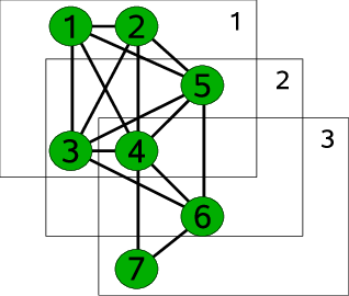
We consider a given set of cliques containing sites each, an instantiation of a certain clique distribution . We presume the clique-set to be monotonically ordered,
| (1) |
as illustrated in Fig. 1. We study the task to generate recursively a dense and connected graph out of the cliques in such a way that the final graph has exactly the same distribution of fully connected subgraphs, viz of cliques. In Fig. 1 we illustrate the simplest procedure for solving this task, by concatenating the cliques via a single common vertex between two consecutive cliques.
Let us shortly digress and consider what would have happened if we had used sites 4 and 7, together with a new site 9 to attach the clique in the third step for the case illustrated in Fig. 1. In this case sites 4 and 7 would be connected and a spurious 3-site clique, namely (4,5,7), would have been generated. A thoughtless attachment of cliques in general therefore generates spurious additional cliques, resulting in an uncontrolled clique distribution for the final graph.

II.1 Hierarchical algorithm
In general one can join two cliques of sizes and via common vertices. The minimal number of common vertices is one, the maximal is
| (2) |
Using more common sites, namely , would result in the destruction of the smaller clique. We can then formulate a class of hierarchical algorithms conserving a given, arbitrary but ordered, via (1), initial clique distribution:
- [1
-
] At step one adds the clique with sites. One starts by selecting a number . Here we will mostly concentrate on the case .
- [2
-
] Next one selects recursively mutually interconnected vertices out of the graph segment constructed in the previous steps. The new clique is then added by mutually connecting new sites among themselves and with the selected sites of the existing graph segment.
We call the choice the ‘dense hierarchical algorithm’; it is illustrated in Fig. 2. Here we will study exclusively the dense algorithm, which results in quite dense networks. The opposite limit, namely the case in step [1] of the hierarchical algorithm, is illustrated in Fig. 1.
Starting with cliques the dense hierarchical algorithm generates a network containing sites in its final state, with
| (3) |
with being the size of the starting clique, which is also the largest. This is so, because exactly one new vertex is added at each of the steps.
II.2 Random vs. preferential attachment
The selection of the vertices in step [2] can be done either randomly, by preferential attachment or other rules. When considering preferential attachment we first select a single vertex with an attachment probability proportional to the vertex-degree ,
| (4) |
(linear preferential attachment). We then select recursively vertices out of the neighbors of via preferential attachment. The set of possible vertices is given, at every step of this recursive selection process, by the set of vertices linked to all sites previously selected. Note that the ordering (1) of the initial clique distribution is a precondition for the hierarchical algorithm to function.
II.3 Decimation algorithm
For further reference we shortly mention a second clique-conserving algorithm for network construction via vertex decimation. Starting with an initial network of unconnected cliques one selects pairs of unconnected vertices either randomly or via preferential attachment. One then attempts a decimation by merging the two selected vertices into a single vertex. One then calculates the clique distribution of the new network which has one less site. If the new clique distribution is identical to the original distribution the decimation is accepted, or else it is rejected.

III Simulation results
We have studied the properties of the hierarchical clique-conserving graph-generation algorithm extensively using numerical results, evaluating their respective statistical properties and comparing them to some selected real-world graph.
III.1 Initial clique distribution
The hierarchical graph generation algorithm, conserves per construction the initial clique distribution . We have studied two cases. In Sect. IV we will discuss the results obtained by using the measured clique distribution of real-world networks for . Here we will concentrate on some of the model clique distributions, in particular of scale-free form
| (5) |
We performed simulations for various exponents , and scale-free clique-distributions containing a total number of cliques. For the simulations a cut-off needs to be chosen for the scale-free distribution (5), i.e. the maximal clique-size . The expected number of cliques is then
| (6) |
where is the total number of cliques. We selected by the condition
| (7) |
viz that there is at least one clique of size present on the average. We compared results obtained for ranging typical from , in order to extract scaling properties in the large-network limit. In order to extract reliable statistical properties the results were averaged over different random realizations.
When selecting the value for the maximal clique size one discards all cliques with sizes . This is admissible when the percentage of discarded cliques is small. With the criteria (7) the percentage of discarded cliques vanishes in the thermodynamic limit . For the system of order , the percentage of discarded is well below .
| 0.34 | 3.2 | 7.5 | 5.1 | 0.00508 | 1007 | -2.6 | |
| 0.36 | 3.3 | 8.8 | 5.7 | 0.00056 | 10032 | -2.7 | |
| 0.37 | 3.4 | 9.8 | 5.8 | 0.000058 | 100096 | -2.4 |

III.2 System-size analysis
In Fig. 3 we present the degree distribution for graphs with a scale-free clique distribution (5) and an exponent , generated through the hierarchical algorithm with preferential attachment. The degree distribution results from averaging realizations for clique distributions containing cliques. We note that the degree distribution approaches a well defined curve for the thermodynamic limit .
The degree distributions shown in Fig. 3 have bumps at high degrees for finite numbers of cliques . This is due to the fact that the algorithm starts by incorporating the large cliques first so that vertices with an high initial degree see it further increased via the preferential attachment during the construction process. This effect vanishes in the thermodynamical limit as the probability of a given vertex to be chosen as a part of a new clique decreases with system size.
The statistical analysis of the networks presented in Fig. 3 are given in Table 1, the number of cliques and the number of vertices, obey the relation (3) valid for the dense hierarchical algorithm. The resulting degree distribution, approaches within the numerical errors, a scale-free functional dependence with an exponent approximately given by the exponent of the conserved clique distribution .
In Fig. 4 we compare the degree distribution between construction rules with preferential and random attachment respectively. The difference is quite small in the region of small to intermediate degrees , where the finite-size corrections are minor, the reason being the algorithmic restriction, that only common neighbors of the already processed vertices can be used to construct a clique iteratively. This restriction decreases the number of vertices available for the preferential attachment and results in a similar degree distribution, which is however slightly different from the ideal scale free line.

III.3 Dependency on the scaling exponent
We have studied the properties of the graphs generated by the hierarchical algorithm for scale-free clique distributions and several scaling exponents . We have analyzed the corresponding graphs as a function of clique-numbers , averaging over several clique-distribution realizations. The resulting degree distributions are shown in Fig. 5 for the case , the corresponding statistical analysis in Table 2. In order to estimate the finite-size corrections we present in Table 3 the corresponding results for . We note, in particular, a good agreement in the estimates for the scaling exponent of the resulting degree distribution.
Interestingly enough, the exponent for the degree distribution of the graph generated by the hierarchical algorithm with preferential attachment saturates at , close to the value expected for the standard preferential attachment algorithm [1]. When the large tail of the degree distribution stemming directly from the clique distribution dominates the resulting exponent for the degree distribution, but fails to do so for , when the preferential attachment mechanism dominates the generation of the fat tail.
Next, we comment on the size of the network diameter of the generated graphs. With increasing we observe an increasing average path length and an increasing average diameter while the clustering coefficient decreases. The network diameter is intuitively affected by the number of low-degree vertices. A larger number of low-degree vertices for degree distributions of identical functional dependences, generally results in a bigger network diameter. Alternatively one may consider the number of trivial cliques, namely those with size , viz edges not forming part of any larger clique. They tend to connect to low-degree vertices, since two connected high-degree vertices would have a higher probability to belong to cliques of size 3 or larger.
| 2.1 | 0.51 | 3.2 | 9.2 | 9.9 | 0.000098 | 100099 | -2.1 |
| 2.6 | 0.36 | 3.4 | 9.8 | 5.8 | 0.000058 | 100096 | -2.4 |
| 3.2 | 0.23 | 3.7 | 11.3 | 3.8 | 0.000038 | 100042 | -3.1 |
| 4.2 | 0.10 | 4.1 | 13.4 | 2.8 | 0.000027 | 100020 | -3.2 |
In order to examine the influence of these trivial cliques on the network diameter we have eliminated, from the graph generated by the hierarchical algorithm with and all cliques of size . The statistical properties of the resulting graph are given in Table 3. The network diameter decreases substantially and the clustering increases. We note that the scaling exponent for the degree distribution remains unaffected, as it depends on the vertices with large degrees only. This result is nevertheless somewhat surprising, in view of dramatic reduction in the number of vertices resulting from the decimation of all trivial cliques.
Right table: The same data as for the left table, but with all cliques of degree removed from the graphs.
N 2.1 0.51 3.1 7.5 10.5 0.00104 10093 -2.0 2.6 0.36 3.4 8.8 5.6 0.00056 10032 -2.5 3.2 0.23 3.7 10.0 3.8 0.00038 10017 -2.9 4.2 0.10 4.1 11.8 2.7 0.00027 10007 -3.1 N 2.1 0.94 2.73 4.1 16.7 0.0028 5885 -2.0 2.6 0.92 2.77 4.5 10.0 0.0021 4625 -2.5 3.2 0.90 2.77 4.9 7.2 0.00206 3491 -3.0 4.2 0.97 2.74 5.0 5.5 0.0024 2207 -3.0
IV Comparison with real world data
We have evaluated the clique distributions for two real-world networks, a protein-protein interaction network [14] and a WWW-graph [12]. We then have used the resulting clique distributions , as the starting point for the hierarchical algorithm with preferential attachment and compared the hence generated graphs with the properties of the original real-world networks.
Fig. 6 shows the clique and the degree distributions of the respective original graphs, with their corresponding statistical properties given in the Table 4. We note that the protein-interaction graph contains cliques of up-to ten sites, where a typical clique-size is slightly larger in the WWW-net. The scaling of the degree distribution is clearly observable for the WWW-net, but only indicative for the protein-interaction networks, due to the limited number of vertices it contains.


Right figure: Degree distribution of the same data shown in left figure. Continuous lines show the respective slope of , . The statistical properties are given in Table 4
In Table 4 we have also included the properties of the graphs generated by the hierarchical algorithm using preferential attachment. The main difference between the generated networks analyzed in Table 4 and those previously discussed, is the fact that they are not averaged over an ensemble of realizations of a clique distribution. The reason is, that the exact experimental clique distributions for the protein-interaction network and for the WWW-network have been taken as an input for the hierarchical algorithm, which is per construction conserved with respect to the clique distribution.
Next we note two caveats with respect to the protein interaction graph. Firstly, it is not complete, being updated continuously as new experimental results become available [14]. Secondly, the protein-interaction network contains unconnected subsets of vertices. The largest component does not encompass the entire graph but 8972 sites out of a total of 9362 vertices. We have used this largest component for the data analysis.
While analyzing the data presented in Table 4 we note substantial differences between the properties of the real-world graphs with respect to the one generated by the hierarchical clique-conserving algorithm. These differences involve essentially all key statistical quantities, such as the total number of vertices, the average degree, the network diameter and the large-k falloff of degree distribution.
This leaves us with two possible conclusions, the first being that the clique distribution is probably not a good quantity for the purpose of characterizing a given graph, at least in the two examples considered here. The second is the possibility that an altogether different clique-conserving algorithm may be needed for the clique distribution to be used as a characterizing quantity.
The data presented in Table 4 was generated using the hierarchical algorithm with preferential attachment, however, as discussed above (see Fig. 4), the difference between random and preferential attachment is actually quite small for clique distributions having a fat tail.
| data | source | N | ||||||
|---|---|---|---|---|---|---|---|---|
| real | 0.11 | 4.3 | 14 | 7.8 | 0.00085 | 8972 | -2.5 | |
| HPPI | gener. | 0.20 | 3.8 | 11 | 3.0 | 0.00016 | 25747 | -3.5 |
| real | 0.23 | 7.2 | 46 | 3.0 | 0.000009 | 325729 | -2.8 | |
| WWW | gener. | 0.27 | 3.751 | 12 | 4.1 | 0.0000086 | 475588 | -3.6 |
V Discussion
In this paper we presented an algorithm, the hierarchical algorithm, by which one can generate graphs having a pre-determined distribution of cliques, viz of fully connected subgraphs. We have studied, in a first step, the degree distribution of the resulting networks for scale-free clique distribution as a function of the scaling exponent.
In a second step we used two selected real-world graphs, a protein-interaction network and a WWW-network, and examined the relation between their degree and clique distributions relative to those of graphs generated via the hierarchical algorithm having the same respective clique distribution. We find no good agreement, and this leads us to the conclusion that either the clique distribution is insufficient for a in-depth characterization of real-world networks or that the hierarchical algorithms need further development.
References
- [1] R. Albert and A. Barabàsi, “Statistical mechanics of complex networks”, Reviews of Modern Physics 74, 47 (2002).
- [2] S.N. Dorogovtsev and J.F.F. Mendes, “Evolution of networks” Advances in Physics 51, 1079 (2002).
- [3] C. Gros, “Complex and Adaptive Dynamical Systems, A Primer”, Springer (2007, in press).
- [4] P. Erdös and A. Rényi, “On random graphs” Publicationes Mathematicae 6, 290 (1959).
- [5] M.E.J. Newman, S.H. Strogatz and D.J. Watts, “Random graphs with arbitrary degree distributions and their applications”, Phys. Rev. E 64, 026118 (2001).
- [6] G. Palla, I. Derenyi, I. Farkas and T. Vicsek, “Uncovering the overlapping community structure of complex networks in nature and society” Nature 435, 814 (2005).
- [7] R. Milo et al. “Network Motifs: Simple Building Blocks of Complex Networks” 298 824 (2002).
- [8] A. Vazquez, R. Dobrin, D. Sergi, J.-P. Eckmann, Z.N. Oltvai and A.-L. Barabasi, “The topological relationship between the large-scale attributes and local interaction patterns of complex networks”, Proc. Nat. Acad. Sci. 101, 17940 (2004).
- [9] S.N. Dorogovtsev, A.V. Goltsev and J.F.F. Mendes, “k-Core Organization of Complex Networks”, Phys. Rev. Lett. 96, 040601 (2006).
- [10] I. Derenyi, G. Palla and T. Vicsek, “Clique percolation in random networks” Phys. Rev. Lett. 94, 160202 (2005).
- [11] G. Bianconi and M. Marsili, “Emergence of large cliques in random scale-free networks”, Europhys. Lett. 74 740 (2006).
- [12] R. Albert, H. Jeong, A.-L. Barabási, “Diameter of the world-wide web” Nature 401, 130 (1999).
- [13] L. Laura, S. Leonardi, G. Caldarelli, P. De Los Rios,”A Multi-Layer Model for the Web Graph”, 2002
- [14] S. Mathivanan et al. “An evaluation of human protein-protein interaction data in the public domain”, BMC Bioinformatics 7 (Suppl 5), S19 (2006).