On the Optimization of the IEEE 802.11 DCF: A Cross-Layer Perspective
Abstract
This paper is focused on the problem of optimizing the aggregate throughput of the Distributed Coordination Function (DCF) employing the basic access mechanism at the data link layer of IEEE 802.11 protocols. In order to broaden the applicability of the proposed analysis, we consider general operating conditions accounting for both non-saturated and saturated traffic in the presence of transmission channel errors, as exemplified by the packet error rate .
The main clue of this work stems from the relation that links the aggregate throughput of the network to the packet rate of the contending stations. In particular, we show that the aggregate throughput presents two clearly distinct operating regions that depend on the actual value of the packet rate with respect to a critical value , theoretically derived in this work.
The behavior of paves the way to a cross-layer optimization algorithm, which proved to be effective for maximizing the aggregate throughput in a variety of network operating conditions. A nice consequence of the proposed optimization framework relies on the fact that the aggregate throughput can be predicted quite accurately with a simple, yet effective, closed-form expression, which is also derived in the article.
Finally, theoretical and simulation results are presented throughout the work in order to unveil, as well as verify, the key ideas.
Index Terms:
Cross-layer, DCF, distributed coordination function, IEEE 802.11, MAC, non-saturated, optimization, saturation, throughput, unloaded traffic, unsaturated.I Introduction
DCF represents the main access mechanism at the Medium Access Control (MAC) layer [1] of the IEEE802.11 series of standards, and it is based on Carrier Sense Multiple Access with Collision Avoidance (CSMA/CA).
Many papers, following the seminal work by Bianchi [2], have addressed the problem of modeling, as well as optimizing, the DCF in a variety of traffic load models and transmission channel conditions.
Let us provide a survey of the recent literature related to the problem addressed in this paper. Papers [3]-[7] model the influence of real channel conditions on the throughput of the DCF operating in saturated traffic conditions. Paper [3] investigates the saturation throughput of IEEE 802.11 in presence of non ideal transmission channel and capture effects.
The behavior of the DCF of IEEE 802.11 WLANs in unsaturated traffic conditions has been analyzed in [8]-[13], whereby the authors proposed various bi-dimensional Markov models for unsaturated traffic conditions, extending the basic bi-dimensional model proposed by Bianchi [2]. In [14], the authors look at the impact of channel induced errors and of the received Signal-to-Noise ratio (SNR) on the achievable throughput in a system with rate adaptation, whereby the transmission rate of the terminal is modified depending on either direct, or indirect measurements of the link quality.
The effect of the contention window size on the performance of the DCF has been investigated in [15]-[22] upon assuming a variety of transmission scenarios. In [15]-[17], the authors addressed the optimization of the contention window in such a way as to optimize the saturated throughput of the DCF.
As a starting point for the derivations which follow, we adopt the bi-dimensional model proposed in a companion paper [12] (see also [13]). Briefly, in [12] the authors extended the saturated Bianchi’s model by introducing a new idle state, not present in the original Bianchi’s model, accounting for the case in which the station queue is empty. The Markov chain of the proposed contention model was solved for obtaining the stationary probabilities, along with the probability that a station starts transmitting in a randomly chosen time slot.
In this paper the focus is different in many respects. Firstly, we investigate the behavior of the aggregate throughput as a function of the traffic load of the contending stations, and note that the aggregate throughput presents two distinct operating regions identified, respectively, by Below Link Capacity (BLC) region and Link Capacity (LC) region. Derived in closed-form in this work, and identified by throughout the paper, the link capacity of the considered scenario corresponds to the maximum throughput that the network can achieve when the contending stations transmit with a proper set of network parameters. We show that the network operates in the BLC region when the actual value of the packet rate is less than a critical value , theoretically derived in this work.
The second part of this article is focused on the optimization of the DCF throughput. We propose a cross-layer algorithm whose main aim is to allow the network to operate as close as possible to the link capacity . The proposed optimization algorithm relies on a number of insights derived by the behavior of the aggregate throughput as a function of the traffic load , and aims at choosing either an appropriate value of the minimum contention window , or a proper size of the transmitted packets depending on the network operating region.
Finally, we derive a simple model of the optimized throughput, which is useful for predicting the aggregate throughput without resorting to simulation.
The rest of the paper is organized as follows. Section II briefly presents the Markov model at the very basis of the proposed optimization framework, whereas Section III investigates the behavior of the aggregate throughput as a function of the traffic load . The proposed optimization algorithm is discussed in section IV. Section V presents simulation results of the proposed technique applied to a sample network scenario, while Section VI draws the conclusions.
II Markov Modeling
The bi-dimensional Markov Process of the contention model proposed in [12], and shown in Fig. 1 for completeness, governs the behavior of each contending station through a series of states indexed by the pair whereby identifies the backoff stage. On the other hand, the index , which belongs to the set , identifies the backoff counter. By this setup, the size of the th contention window is while is the minimum size of the contention window.
An idle state, identified by in Fig. 1, is introduced in order to account for the scenario in which after a successful transmission there are no packets to be transmitted, as well as for the situation in which the packet queue is empty and the station is waiting for a new packet arrival.
The proposed Markov model accounts for packet errors due to imperfect channel conditions, by defining an equivalent probability of failed transmission, identified by , which considers the need for a new contention due either to packet collisions () or to channel errors () on the transmitted packets, i.e.,
| (1) |
It is assumed that at each transmission attempt each station encounters a constant and independent probability of failed transmission, independently from the number of retransmissions already suffered.
The stationary solution of the Markov Model in Fig. 1 is employed to compute , the probability that a station starts a transmission in a randomly chosen time slot. First of all, observe that a packet transmission takes place when a station goes in one of the states . Therefore, the probability can be evaluated by adding up the probabilities over the set . Upon imposing the normalization condition11 1 The probabilities must add up to , and . on the Markov model in Fig. 1, and expressing the probabilities as a function of the probabilities , the probability can be rewritten as follows:
| (2) |
As in Bianchi’s work [2], we assume that: 1) the probability is constant across all time slots; 2) the probability is constant and independent of the number of collisions already suffered.
Given , the probability of collision , can be defined as follows:
| (3) |
Finally, the term in (2) is the probability of having at least one packet waiting for transmission in the station queue after an average slot duration.
Let us spend few words on the evaluation of . Upon assuming that the packet interarrival times are exponentially distributed with mean22 2 , which is measured in , represents the rate at which the packets arrive into the station queue from the upper layers. , the probability can be well approximated by the following relation in a scenario where the contending stations employ queues of small sizes [9]:
| (4) |
where , the expected time per slot, is useful to relate the states of the Markov chain to the actual time spent in each state. As a note aside, notice that in (4) corresponds to the probability that zero packets are received from the upper layers when the packet interarrival times are exponentially distributed.
The other terms involved in are defined as follows [2, 12]. is the duration of an empty time slot; is the probability that there is at least one transmission in the considered time slot, with stations contending for the channel, each transmitting with probability ; is the conditional probability that a packet transmission occurring on the channel is successful; , and are, respectively, the average times a channel is sensed busy due to a collision, the transmission time during which the data frame is affected by channel errors, and the average time of successful data frame transmission.
III Throughput Analysis
The computation of the normalized system throughput relies on the numerical solution of the nonlinear system obtained by jointly solving (1) and (2). The solution of the system, which corresponds to the values of and , is used for the computation of the normalized system throughput, i.e., the fraction of the time during which the channel is used to successfully transmit payload bits:
| (5) |
whereby is the average packet payload length, and can be rewritten as [2]:
| (6) |
In order to gain insights on the behavior of the aggregate throughput , let us investigate the theoretical behavior of (5) as a function of the packet rate for two different values of the packet error probability , and minimum contention window , in a scenario with contending stations transmitting at the bit rate Mbps.
The two rightmost subplots of Fig. 2 show the theoretical behavior of the throughput in (5), as well as simulation results obtained with NS2 by employing the typical MAC layer parameters for IEEE802.11b given in Table I [1]. Other parameters are noticed in the label of the figure. Let us spend a few words about the simulation setup in ns-2. In order to account for imperfect channel transmissions, the channel model is implemented using the suggestions proposed in [23], where the outcomes of a binary, equiprobable random variable are used to establish whether each packet is received erroneously. In other words, the random variable is equal to with probability (erroneous transmission), and with probability . We notice in passing that the theoretical model developed is independent on the specific propagation channel. The only parameter needed is , which can be appropriately linked to the specific wireless propagation channel upon specifying a threshold of the signal-to-noise ratio allowing perfect reception at the receiver [24].
We adopted the patch NOAH (NO Ad-Hoc), available on the authors’ website33 3 See http://icapeople.epfl.ch/widmer/uwb/ns-2/noah/, for emulating a wireless network in infrastructure mode.
The employed traffic model is implemented by generating an exponentially distributed random variable with expected value , in accordance to the theoretical model developed in Section II.
Let us focus on the curves noticed in the two rightmost subplots in Fig. 2. Basically, there are two different operating regions of the throughput in (5). As , i.e., all the contending stations approach unloaded traffic conditions, the throughput can be approximated as a straight line passing through the point :
| (7) |
This relation follows from the theoretical throughput noticed in (5) upon approximating the probabilities and in the limit .
Indeed, as , the first relation in (4) yields , whereas the probability in (2) can be well approximated by . Since as (because ), it is . Furthermore, as , (6) can be approximated by the following relation:
| (8) |
Upon substituting (8) in (5), the theoretical throughput can be well approximated as follows:
| (9) | |||||
This linear model is depicted in the subplots of Fig. 2 overimposed to both theoretical and simulated results. The key observation from this result is that the aggregate throughput produced by stations approaching unloaded traffic conditions, is only dependent on the number of stations, as well as on the packet size. No other network parameters affect the aggregate throughput in this operating region. Moreover, the results depicted in Fig. 2 denote that the derived linear model is valid up to a critical value of (identified by throughout the paper), above which the aggregate throughput no longer increases linearly with . We note in passing that, given , there is no need to simulate the network to obtain the aggregate throughput: it is very well approximated by the theoretical relation derived in (9) for any .
Once again, let us focus on the results shown in the rightmost subplots of Fig. 2. The aggregate throughput gets to a maximum at a proper value of , above which the effect of the collisions among the stations, as well as the propagation channel, let the throughput reach a horizontal asymptote. The maximum value of over the whole range of values of turns to be quite useful for throughput optimization. Obtained by Bianchi [2] under the hypothesis of saturated network, and considering only collisions among the stations, in our more general model such a maximum can be estimated in two steps. First, rewrite the throughput in (5) as a function of by using the relations that define and in terms of the probability . Then, equate to zero the derivative of the throughput in (5) with respect to , and obtain a solution identified by . By doing so, the value of for which the throughput gets maximized is easily obtained:
| (10) |
Finally, evaluate the throughput in (5) on the solution noticed in (10). Upon following these steps, the maximum throughput takes on the following form
| (11) |
The critical value of acts as a transition threshold between two operating regions. In the first region, i.e., for , the transmissions are affected by relatively small equivalent error probabilities, . In this operating region44 4 In what follows, this operating region will be identified by the acronym BLC, short for Below Link Capacity region., collisions among stations occur rarely ( is small) because of the reduced traffic load of the contending stations, and the stations experience good channel quality ( is very small). For any , the network is not congested, and the contending stations are able to transmit data below the link capacity limit denoted by . This is the reason for which the aggregate throughput grows linearly with the traffic load .
On the other hand, the aggregate throughput tends to be upperbounded by in (11) for . The reason is simple: the aggregate throughput in this region55 5 In what follows, this operating region will be identified by the acronym LC, short for Link Capacity region. is affected either by the increasingly effects of the collisions among the stations, or by worse channel conditions as exemplified by . Further insights on this statement can be gained by the results discussed below in connection with the curves shown in Fig. 4.
The critical value of can be found as the abscissa where the linear model of the throughput in (7) equates to in (11):
| (12) |
The procedure for obtaining , is clearly highlighted in all the four subplots of Fig. 2.
Let us investigate the behavior of the critical value in (12) against some key network parameters.
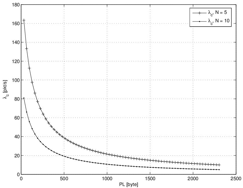
Fig. 3 shows the behavior of as a function of the packet size , for two different values of as noticed in the respective legends. Some observations are in order. decreases for longer packet sizes , as well as for increasing number of contending stations, . The reason relies on the fact that for increasing packet sizes, each station tends to occupy the channel longer. Such a behavior is clearly emphasized in Fig. 4, where the aggregate throughput for a sample scenario comprising 10 contending stations transmitting with the packet sizes noticed in the legend, is considered.
As long as the packet size increases, the aggregate throughput shows an increasing slope in the linear region characterized by traffic loads , as suggested by the theoretical model in (9). Moreover, the value of tends to decrease because each station tends to occupy the channel longer. The three lower thick curves, labeled by bytes, are associated to three different values of packet error probabilities, . Note that the value of decreases for increasing values of , thus reducing the region characterized by small equivalent error probabilities. As long as , both and tend to zero, making the aggregate throughput vanishingly small.
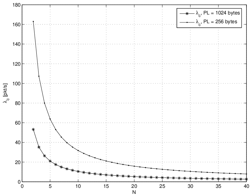
Similar considerations may be derived from the behavior of versus noticed in Fig. 5. Roughly speaking, for fixed values of the packet size, tends to reduce by a half as far as the number of contending stations doubles. The reason relies on the fact that the probability of collision increases as long as more stations try to contend for the channel.
IV Throughput Optimization
The considerations deduced in Section III are at the very basis of an optimization strategy for maximizing the aggregate throughput of the network depending on the traffic load . To this end, we define two optimization strategies: Contention Window Optimization and MAC Payload Size Optimization. The first strategy is applied when the contending stations operate in the LC region, approaching the link capacity , whereas the second one is used for optimizing the aggregate throughput when the stations operate within the BLC region.
The next two subsections address separately the two optimization strategies, while Section V presents the optimization algorithm jointly implementing the two strategies.
IV-A Link Capacity region: Contention Window Optimization
The first optimization strategy proved to be effective for improving the aggregate throughput in the LC region, i.e., for . The key idea here is to force the contending stations to transmit with a probability equal to the one that maximizes the aggregate throughput . In this respect, the probability in (10) plays a key role.
Upon considering saturated conditions, i.e., imposing in (2), the probability can be rewritten as:
| (13) |
By substituting in (3), can be rewritten as:
| (14) |
whereby .
Finally, by equating (13) to in (10), and solving for , we obtain the optimal minimum contention window size in terms of the key network parameters:
| (15) |
This relation yields the value of the minimum contention window that maximizes the aggregate throughput when the number of contending stations , the packet error rate over the channel , and the number of backoff stages , are given. As a note aside, notice that, using , the maximum throughput equates to the link capacity in (11).
Moreover, we notice that for , i.e., no exponential backoff is employed, in (15) can be simplified as follows:
Considering as a function of , and neglecting the multiplicative constant terms, it is simple to notice that in (10) goes roughly as when . Therefore, the optimal contention window grows linearly with the number of contending stations (when ) in order to mitigate the effects of the collisions due to an increasing number of contending stations in the network.
In the following, we present simulation results accomplished in NS-2 for validating the theoretical models, as well as the results presented in this section. The adopted MAC layer parameters for IEEE802.11b are summarized in Table I [1].
The main simulation results are presented in Figs. 2 and 6 in connection to the set of parameters noticed in the respective labels.
Some observations are in order. Let us focus on the results shown in Fig. 2. A quick comparison among the leftmost and the rightmost subplots of Fig. 2 reveals that the choice in (15) guarantees improved performance for any , thus making the aggregate throughput equal . Throughput penalties due to the use of an suboptimal , are in the order of kbps.
Notice also that the value of is independent from the minimum contention window chosen.
The key observation from the subplots of Fig. 2 concerns the fact that the aggregate throughput of the optimized network can be modeled as follows:
As emphasized by the curves in Fig. 2, this model shows a very good agreement with both theoretical and simulation results. Once again, notice that the aggregate throughput may be predicted quite accurately without resorting to simulation.
Let us focus on the results shown in Fig. 6, where the saturation throughput represented by continuous curves, is derived as a function of the minimum contention window size . The curves are parameterized with respect to the three different values of noticed in the legend. The simulated scenario considers contending stations transmitting packets of size bytes. Shown in the same figure is the theoretical throughput in (5) represented by dashed curves.
The saturation throughput in each simulated scenario reaches a maximum corresponding to the abscissas predicted by (15) and noticed beside each maximum. We notice that tends to be quite insensitive from the packet error rate , whose main effect corresponds to a reduction of the maximum achievable throughput.
IV-B Below Link Capacity region: Payload Size Optimization
The analysis of the aggregate throughput in Section III revealed the basic fact that for traffic loads less than , the network is not congested, and each station achieves a throughput roughly equal to (the aggregate throughput is thus ). We note in passing that the throughput does not depend on the minimum contention window in the LC region. Therefore, given contending stations, the throughput can only be improved by increasing the payload size when the traffic load satisfies the relation .
Before proceeding any further, let us discuss two important issues in connection with the choice of the packet size .
As long as the erroneous bits are independently and identically distributed over the received packet66 6 We notice that wireless transceivers make use of interleaving in order to break the correlation due to the frequency selectivity of the transmission channel [24]., the packet error probability can be evaluated as
| (16) |
where,
| (17) |
and
| (18) |
In the previous relations, and are, respectively, the sizes (in bits) of the MAC and PLCP77 7 PLCP is short for Physical Layer Convergence Protocol. headers, and is the size of the data payload in bits. Equ. (18) accounts for the fact that a packet containing the useful data, is considered erroneous when at least one bit is erroneously received. Relation (16) is obtained by noting that a packet is received erroneously when the errors occur either in the PLCP part of the packet, or in the information data.
We notice that the relations (16) through (18) are valid either with the use of convolutional coding, whereby the bit error rate performance does not depend on the code block size [24], or for protocols that do not employ channel encoding at the physical layer.
From (18) it is quite evident that the higher the payload size, the higher the packet error rate; and viceversa. As a note aside, we notice that this behavior does not hold when concatenated convolutional channel codes [25]-[27], as well as low-density parity-check codes, are employed as channel codes. Indeed, for these codes the packet error rate depends on the size of the encoded block of data, with longer packets having smaller probability of error compared to shorter packets.
The second issue to be considered during the choice of is related to the critical value , which depends on the packet error probability ( defined in (16)), and consequently on the payload size. Given a traffic load , any change in could affect the network operating region, which might move from the BLC region to the LC region.
Let us discuss a simple scenario in order to reveal this issue88 8 Where not otherwise specified, we employ the network parameters summarized in Table I.. Consider a network (identified in the following as scenario A) where contending stations with traffic load pkt/s transmit packets of size bytes. Assume that the bit error probability due to the channel conditions is , which corresponds to a packet error rate (from (16)). Upon using the network parameters summarized in Table I, the critical load in (12) corresponds to pkt/s. Since , the network is in the BLC operating region. If the stations increase the payload size up to bytes, the packet error rate increases to the value , with the side effect of decreasing to pkt/s. Therefore, for the given traffic load pkt/s, the network starts operating into the LC region.
Based on the considerations deduced in the scenario A, the proposed optimization technique aims to optimize the payload size in two consecutive steps. In the first step, we find the size of the payload in such a way that the critical threshold equals the actual traffic load , in order for the network not to operate beyond the BLC region.
The second step verifies whether the packet error rate associated to this payload size, is below a predefined PER-target (identified by PERt), which defines the maximum error level imposed by the application layer. First of all, given an estimated bit error probability at the physical layer, solve (18) for . Then, solve (16) for , and substitute the relation in place of . Considering PERt, the following maximum payload size follows:
| (19) |
whereby is the ceil of the enclosed number.
Let us consider again the scenario A discussed previously with the application of this algorithm. Consider stations transmitting packets of size bytes at the traffic load pkt/s. Assume that the bit error rate imposed by the specific channel conditions is , yielding and pkt/s. Moreover, assume a target PER equal to99 9 This is the maximum PER specified in the IEEE 802.11b standard [1], guaranteed at the receiver when the received power reaches the receiver sensitivity. PER.
Since , after the first step, the algorithm selects the optimal size bytes, which moves the working point near the link capacity and leads to the actual packet error rate . Since the constraint PERt is not satisfied, the proposed method estimates the size in order to attain the PERt constraint. The packet size becomes eventually bytes (from (19)), yielding a packet error rate and a pkt/s, thus leaving the working point in the BLC region.
Finally, the optimal payload size is:
where bytes is the maximum packet size imposed by the standard [1].
Simulation results of a sample network employing the algorithm described above, are presented in the next section, along with a sample code fragment summarizing the key steps of the optimization technique.
V Simulation Results
In this section, we present simulation results for a network of contending stations, employing the optimization strategies described in Section IV.
The basic steps of the proposed optimization algorithm are summarized in Table II. Let us spend a few words about the implementation of the proposed algorithm in a WLAN setting employing the infrastructure mode, where an Access Point (AP) monitors the transmissions of contending stations.
The evaluation of the critical value in (12) requires the estimation of three key parameters of the network: the number of contending stations , the packet error rate , and the value of the optimal , which depends on . Each station can estimate the number of contending stations by resorting to one of the algorithms proposed in [28]-[30]. On the other hand, the packet error probability , may be evaluated through (16), once the bit error probability at the physical layer is estimated. We recall that can be estimated by employing proper training sequences at the physical layer of the wireless receiver [24].
Finally, the value of the optimal can be evaluated by each station with the parameters and . A similar reasoning applies for the estimation of the optimal packet size.
We have realized a C++ simulator implementing all the basic directives of the IEEE 802.11b protocol with the 2-way handshaking mechanism, namely exponential backoff, waiting times, post-backoff, and so on. In our simulator, the optimization algorithm is dynamically executed for any specified scenario. For the sake of analyzing the effects of the optimization, the instantaneous network throughput is evaluated over the whole simulation. The aggregate throughputs obtained in the investigated scenarios are shown in Fig. 7.
In the first scenario, we considered a congested network in which 10 stations transmit packet of fixed size bytes at the packet load pkt/s and bit rate 1 Mbps. Other parameters are , and , whereas the channel conditions are assumed to be ideal. As shown in Fig. 7 (curve labeled LC region with asterisk-marked points), the aggregate throughput is about bps. After s, out of the stations turn their traffic off. Between 40s and 80s, the aggregate throughput increases to about bps because of the reduced effect of the collisions among the contending stations. After s, the stations turn on again and the aggregate throughput decreases to bps.
Consider again the same scenario over a time interval of s, whereby the contending stations adopt the optimal contention window. Upon using (15), the optimal contention window is when 10 stations transmit over the network, and during the interval in which only 5 stations contend for the channel.
The aggregate throughput in the optimized scenario is about bps, as noticed by the star-marked curve in the same figure. We notice that the optimized throughput is quite constant over the whole simulation independently on the number of contending stations in the network, approaching the theoretical maximum throughput bps obtained from (11). Moreover, notice that the two curves related to both and are almost superimposed.
Consider another scenario differing from the previous one in that the contending stations operate in the BLC region. As above, stations contend for the channel in the time intervals s and s, while during the time interval s out of the 10 stations turn off. The traffic load is pkt/s, and the packet inter-arrival times are exponentially distributed.
Let us focus on the aggregate throughput depicted in Fig. 7. The curves related to the scenario at hand are identified by the labels pkt/s. As a result of the application of the proposed algorithm to the choice of the packet size, we obtain bytes for the case when stations are transmitting, and bytes in the other scenario with active stations.
Simulation results show that the proposed algorithm guarantees improved throughput performance on the order of kbps when stations are active, and about kbps when only stations contend for the channel. We notice in passing that, despite the optimization, the aggregate throughput could not reach the maximum because of the low traffic load. Indeed, the capacity link could be achieved by using a packet size longer than either the one imposed by the standard [1], and the value obtained from (19).
For the sake to verify that the optimization of the minimum contention window does not affect the aggregate throughput in the BLC region, Fig. 7 also shows the aggregate throughput obtained by simulation using a minimum contention window equal to . Notice that the related curve is superimposed to the one related to the scenario in which the contending stations employ the minimum contention window suggested by the standard [1].
VI Conclusions
This paper proposed an optimization framework for maximizing the throughput of the Distributed Coordination Function (DCF) basic access mechanism at the data link layer of IEEE 802.11 protocols. Based on the theoretical derivations, as well as on simulation results, a simple model of the optimized DCF throughput has been derived. Such a model turns to be quite useful for predicting the aggregate throughput of the DCF in a variety of network conditions.
For throughput modeling, we considered general operating conditions accounting for both non-saturated and saturated traffic in the presence of transmission channel errors identified by the packet error rate . Simulation results closely matched the theoretical derivations, confirming the effectiveness of both the proposed DCF model and the cross-layer optimization algorithm.
References
- [1] IEEE Standard for Wireless LAN Medium Access Control (MAC) and Physical Layer (PHY) Specifications, November 1997, P802.11
- [2] G. Bianchi, ”Performance analysis of the IEEE 802.11 distributed coordination function”, IEEE JSAC, Vol.18, No.3, March 2000.
- [3] F. Daneshgaran, M. Laddomada, F. Mesiti, M. Mondin, and M. Zanolo, “Saturation throughput analysis of IEEE 802.11 in presence of non ideal transmission channel and capture effects,” to appear on IEEE Trans. on Communications, July 2008.
- [4] Q. Ni, T. Li, T. Turletti, and Y. Xiao, “Saturation throughput analysis of error-prone 802.11 wireless networks”, Wiley Journal of Wireless Communications and Mobile Computing, Vol. 5, No. 8, pp. 945-956, Dec. 2005.
- [5] P. Chatzimisios, A.C. Boucouvalas, and V. Vitsas, “Influence of channel BER on IEEE 802.11 DCF”, IEE Electronics Letters, Vol.39, No.23, pp.1687-1689, Nov. 2003.
- [6] Y. Zheng, K. Lu, D. Wu, and Y. Fang, “Performance analysis of IEEE 802.11 DCF in imperfect channels,” IEEE Transactions on Vehicular Technology, Vol. 55, No. 5, pp. 1648-1656, Sept. 2006.
- [7] H.C. Lee, “Impact of bit errors on the DCF throughput in wireless LAN over ricean fading channels”, In Proc. of IEEE ICDT ’06, 2006.
- [8] L. Yong Shyang, A. Dadej, and A. Jayasuriya, ”Performance analysis of IEEE 802.11 DCF under limited load”, In Proc. of Asia-Pacific Conference on Communications, Vol.1, pp.759 - 763, 03-05 Oct. 2005.
- [9] D. Malone, K. Duffy, and D.J. Leith, ”Modeling the 802.11 distributed coordination function in non-saturated heterogeneous conditions”, IEEE-ACM Trans. on Networking, vol. 15, No. 1, pp. 159-172, Feb. 2007.
- [10] F. Daneshgaran, M. Laddomada, F. Mesiti, and M. Mondin, “On the linear behaviour of the throughput of IEEE 802.11 DCF in non-saturated conditions”, IEEE Communications Letters, Vol. 11, No. 11, pp. 856-858, Nov. 2007.
- [11] G.R. Cantieni, Q. Ni, C. Barakat, and T. Turletti, “Performance analysis under finite load and improvements for multirate 802.11,” Computer Communications, Elsevier, vol.28, No.10, pp.1095-1109, June 2005.
- [12] F. Daneshgaran, M. Laddomada, F. Mesiti, and M. Mondin, “Unsaturated throughput analysis of IEEE 802.11 in presence of non ideal transmission channel and capture effects,” IEEE Trans. on Wireless Communications, Vol. 7, No. 4, pp. 1276-1286, April 2008.
- [13] F. Daneshgaran, M. Laddomada, F. Mesiti, and M. Mondin, “A model of the IEEE 802.11 DCF in presence of non ideal transmission channel and capture effects,” In Proc. of IEEE Globecom 07, Washington DC, November 2007.
- [14] D. Qiao, S. Choi, and K.G. Shin, “Goodput analysis and link adaptation for IEEE 802.11a wireless LANs”, IEEE Trans. On Mobile Computing, Vol.1, No.4, Oct.-Dec. 2002.
- [15] F. Cali, M. Conti, and E. Gregori, ”Dynamic tuning of the 802.11 protocol to achieve a theoretical throughput limit”, IEEE Trans. on Networking, vol. 8, pp. 785799, Dec. 2000.
- [16] A. Khalaj, N. Yazdani, and M. Rahgozar, ”The effect of decreasing CW size on performance in IEEE 802.11 DCF”, Proc. of IEEE ICCN, vol. 1, pp. 521525, Nov. 2005.
- [17] A. Khalaj, N. Yazdani, and M. Rahgozar, “Effect of the contention window size on performance and fairness of the IEEE 802.11 standard”, Wireless Personal Comm., Vol. 43, No. 4, pp. 1267-1278, Dec. 2007.
- [18] S. Choudhury and J. D. Gibson, “Throughput optimization for wireless LANs in the presence of packet error rate constraints”, IEEE Communications Letters, Vol.12, No.1, pp.11-13, January 2008.
- [19] H. Anouar and C. Bonnet, “Optimal constant-window backoff scheme for IEEE 802.11 DCF in single-hop wireless networks under finite load conditions”, Wireless Personal Comm., Vol. 43, No. 4, pp. 1583-1602, Dec. 2007.
- [20] Y. Peng, SD Cheng, and JL Chen, “RSAD: A robust distributed contention-based adaptive mechanism for IEEE 802.11 wireless LANs”, Journal of Computer Science and Technology, Vol. 20, No. 2, pp. 282-288, March 2005.
- [21] Q. Xia and M. Hamdi, “Contention window adjustment for IEEE 802.11 WLANs: A control-theoretic approach”, In Proc. of IEEE ICC 2006, Vol. 9, pp.3923 - 3928, June 2006.
- [22] S. Choudhury and J. D. Gibson, “Payload length and rate adaptation for multimedia communications in wireless LANs”, IEEE JSAC, Vol.25, No.4, pp.796-807, May 2007.
- [23]
Wu Xiuchao, ”Simulate 802.11b channel within NS-2”, available
online at
www.comp.nus.edu.sg/~wuxiucha/research/reactive/report/80211ChannelinNS2_new.pdf - [24] Proakis, J. G., “Digital Communications,” McGraw Hill, Fourth Edition, New York, 2001.
- [25] F. Daneshgaran and M. Laddomada, “Optimized prunable single cycle interleavers for turbo codes,” IEEE Trans. on Communications, vol.52, no.6, pp.899-909, June 2004.
- [26] F. Daneshgaran and M. Laddomada, “Reduced complexity interleaver growth algorithm for turbo codes,” IEEE Trans. on Wireless Communications, vol.4, no.3, pp.954-964, May 2005.
- [27] F. Daneshgaran, M. Laddomada, and M. Mondin, “Interleaver design for serially concatenated convolutional codes: Theory and application,” IEEE Trans. on Information Theory, Vol.50, No. 6, pp. 1177-1188, June 2004.
- [28] A.L. Toledo, T. Vercauteren, and X. Wang, ”Optimizing IEEE 802.11 DCF using bayesian estimators of the network state”, Proc. IEEE ICASSP’05, Vol. 5, 18-23 March 2005, pp. 933-936.
- [29] G. Bianchi and I. Tinnirello, ”Kalman filter estimation of the number of competing terminals in an IEEE 802.11 network”, Proc. IEEE INFOCOM’03, Vol. 2, 30 March-3 April 2003, pp. 844-852.
- [30] K. Jang-Sub, E. Serpedin, and D.-R. Shin, ”Improved particle filtering-based estimation of the number of competing stations in IEEE 802.11 networks”, to appear on IEEE Sign. Process. Letters, pp. 87-90. Available on IEEExplorer.





| MAC header | 24 bytes | Slot time | 20 |
|---|---|---|---|
| PHY header | 16 bytes | SIFS | 10 |
| ACK | 14 bytes | DIFS | 50 |
| s | EIFS | 300 | |
| 32 | ACK timeout | 300 | |
| m | 5 | CTS timeout | 300 |
| 1. | do |
|---|---|
| 2. | Estimation of PER and N |
| 3. | Evaluate from (12) |
| 4. | while(IDLE) |
| 5. | // Request to Send from Upper Layers: |
| 6. | if () |
| 7. | // Link Capacity Operating Region: |
| 8. | The station evaluates from (15) |
| 9. | else |
| 10. | // Below Link Capacity Operating Region: |
| 11. | compute given |
| 12. | compute given |
| 13. | select |
| 14. | end |
| 15. | send packet |