Surface-induced heating of cold polar molecules

Stefan Yoshi Buhmann Affiliation: Quantum Optics and Laser Science, Blackett Laboratory, Imperial College London, Prince Consort Road, London SW7 2AZ, United Kingdom M. R. Tarbutt Affiliation: Quantum Optics and Laser Science, Blackett Laboratory, Imperial College London, Prince Consort Road, London SW7 2AZ, United Kingdom Stefan Scheel Affiliation: Quantum Optics and Laser Science, Blackett Laboratory, Imperial College London, Prince Consort Road, London SW7 2AZ, United Kingdom E. A. Hinds Affiliation: Quantum Optics and Laser Science, Blackett Laboratory, Imperial College London, Prince Consort Road, London SW7 2AZ, United Kingdom

August 24, 2026

Abstract

We study the rotational and vibrational heating of diatomic molecules placed near a surface at finite temperature on the basis of macroscopic quantum electrodynamics. The internal molecular evolution is governed by transition rates that depend on both temperature and position. Analytical and numerical methods are used to investigate the heating of several relevant molecules near various surfaces. We determine the critical distances at which the surface itself becomes the dominant source of heating and we investigate the transition between the long-range and short-range behaviour of the heating rates. A simple formula is presented that can be used to estimate the surface-induced heating rates of other molecules of interest. We also consider how the heating depends on the thickness and composition of the surface.

pacs

34.35.+a 33.80.–b, 37.10.Mn 42.50.Nn,

I Introduction

A number of techniques have recently been developed to cool polar molecules to low temperatures and to trap them for a second or longer. Using the switched electric field gradients of a Stark decelerator [1], polar molecules formed in a supersonic expansion have been decelerated to rest and then stored in electrostatic, magnetic or electrodynamic traps [2, 3, 4, 5]. An electrostatic trap has been continuously loaded by filtering out the slowest fraction of the molecules present in an effusive beam [6]. Polar molecules have also been cooled in a buffer gas of cold helium and then confined in a magnetic trap [7]. Extremely cold polar molecules such as RbCs can be produced by the photoassociation of two species of ultracold atoms, followed by laser-stimulated state transfer [8]. In all cases, the resulting molecules are typically far colder than their environments, and they may be heated by the absorption of blackbody radiation from that environment. Unlike atoms, the polar molecules can be rotationally or vibrationally excited by their interaction with this blackbody radiation, and in many cases this can severely limit the trapping lifetime of the molecules. Indeed, the blackbody heating rate for trapped OH and OD has already been measured experimentally and found to limit the trapping lifetime to just a few seconds when the environment is at room temperature [9]. Calculations of the free-space heating rates for several polar molecules have already been presented [10].

In most experiments so far, the cold polar molecules have been confined in macroscopic traps, with trap surfaces typically several mm from the molecules themselves. There is now a great deal of interest in confining and manipulating these molecules much closer to surfaces, so as to build a ‘molecule chip’ technology analogous to that for atoms [11]. Fast-moving molecules have already been trapped in travelling potential wells formed approximately 25 $\mu$ m above a microstructured surface [12]. This same structure can be used to decelerate the molecules to rest so that they can be trapped above the surface of the chip. Chip-based microtraps have been designed, along with schemes to interface the molecules with solid-state devices which could be used to cool, detect and control them coherently [13]. Strong coupling to a superconducting stripline cavity is possible when the molecules are just a few microns from the surface, and then the molecules can be the long-lived quantum memory of a hybrid quantum information processor [14]. Recent developments also herald the prospect of integrated molecule detectors, based on optical microcavities [15] or ultrathin optical fibers [16].

These advances raise the question of the heating rates in the close vicinity of a surface. The influence of such a non-trivial environment on the internal atomic dynamics is commonly known as the Purcell effect [17]. Early theoretical studies were devoted to the zero temperature case where the evolution is governed by spontaneous decay. As shown by linear response theory, the decay rate for an arbitrary environment can be given in terms of the classical Green tensor for the respective geometry [18]. Alternative approaches have been developed on the basis of classical electrodynamics [19, 20] and microscopic models [21] and have been applied to the case of an atom near a single surface or between two surfaces. Results for an arbitrary environment of electric [22] and magneto-electric bodies [23], including local-field effects [24, 25], have also been obtained on the basis of macroscopic quantum electrodynamics (QED) and have been used to study atoms in bulk material [22], outside [26] or inside a microsphere [24], inside a spherical cavity [27] and even in the presence of left-handed meta-materials [23, 28, 29]. The linear-response approach has been generalised to finite temperatures [30] where the internal dynamics is no longer governed by spontaneous decay alone, but stimulated emission and absorption of thermal photons also contribute. The respective environment-dependent transition rates can again be expressed in terms of the classical Green tensor; in addition, the thermal photon number comes into play. Ground-state heating rates of spinless atoms have been predicted to be very small near surfaces [31], in contrast to the case of atoms with spin which have been investigated for planar surfaces, [31, 32] wires [33] and carbon nanotubes [34].

In this paper, we calculate heating rates for a number of polar molecules currently favoured by experimenters. On the basis of macroscopic QED (presented in Sec. II), we solve the internal molecular dynamics to obtain transition rates of a molecule in an arbitrary uniform-temperature environment (Sec. III). In Sec. IV, the results are first used to calculate the rates in free space, and then as a function of distance from the surface of some common metals and dielectrics, as well as some unusual meta-materials.

II Macroscopic quantum electrodynamics at finite temperature

Consider a molecule (or an atom) that is placed within an arbitrary environment of magneto-electric bodies. The coupled dynamics of the molecule and the body-assisted electromagnetic field can be described by the Hamiltonian [23, 35]

\hat{H}=\hat{H}_{A}+\hat{H}_{F}+\hat{H}_{AF},

(1)

where

\hat{H}_{A}=\sum_{n}E_{n}|n\rangle\langle n|

(2)

( $E_{n}$ , molecular eigenenergies; $|n\rangle$ , molecular eigenstates) is the Hamiltonian of the molecule,

\hat{H}_{F}=\sum_{\lambda=e,m}\int\mathrm{d}^{3}r\int_{0}^{\infty}\mathrm{d}\omega\,\hbar\omega\,\hat{\bm{f}}_{\lambda}^{\dagger}(\bm{r},\omega)\!\cdot\!\hat{\bm{f}}_{\lambda}(\bm{r},\omega),

(3)

is the Hamiltonian of the electromagnetic field (including the internal charges present in the bodies) expressed in terms of the bosonic variables

	$\displaystyle\Bigl[\hat{f}_{\lambda i}(\bm{r},\omega),\hat{f}_{\lambda^{\prime}j}(\bm{r}^{\prime},\omega^{\prime})\Bigr]=0=\Bigl[\hat{f}_{\lambda i}^{\dagger}(\bm{r},\omega),\hat{f}_{\lambda^{\prime}j}^{\dagger}(\bm{r}^{\prime},\omega^{\prime})\Bigr],$		(4)
	$\displaystyle\Bigl[\hat{f}_{\lambda i}(\bm{r},\omega),\hat{f}_{\lambda^{\prime}j}^{\dagger}(\bm{r}^{\prime},\omega^{\prime})\Bigr]=\delta_{\lambda\lambda^{\prime}}\delta_{ij}\delta(\bm{r}-\bm{r}^{\prime})\delta(\omega-\omega^{\prime}),$		(5)

(note that $\hat{\bm{f}}_{e}$ is associated with the polarisation of the bodies and $\hat{\bm{f}}_{m}$ is related to their magnetisation) and

\hat{H}_{AF}=-\sum_{m,n}\bm{d}_{mn}\!\cdot\!\hat{\bm{E}}(\bm{r}_{\!A})\hat{A}_{mn}

(6)

( $\bm{d}_{mn}$ $\!=$ $\!\langle m|\hat{\bm{d}}|n\rangle$ , electric-dipole transition matrix elements of the molecule; $\bm{r}_{\!A}$ , molecular centre-of-mass position; $\hat{A}_{mn}$ $\!=$ $\!|m\rangle\langle n|$ , molecular flip operators) is the molecule–field interaction Hamiltonian in electric-dipole approximation. The electric field can be expressed in terms of the bosonic variables according to

	$\displaystyle\hat{\bm{E}}(\bm{r})=\int_{0}^{\infty}\!\mathrm{d}\omega\,\underline{\hat{\bm{E}}}(\bm{r},\omega)+\operatorname{H.c.},$		(7)
	$\displaystyle\underline{\hat{\bm{E}}}(\bm{r},\omega)=\sum_{\lambda={e},{m}}\int\mathrm{d}^{3}r^{\prime}\,\mbox{{{{G}}}}_{\lambda}(\bm{r},\bm{r}^{\prime},\omega)\!\cdot\!\hat{\bm{f}}_{\lambda}(\bm{r}^{\prime},\omega),$		(8)

with the coefficients $\mbox{{{{G}}}}_{\lambda}$ being related to the classical Green tensor, G, by

		$\displaystyle\mbox{{{{G}}}}_{e}(\bm{r},\bm{r}^{\prime},\omega)=\mathrm{i}\,\frac{\omega^{2}}{c^{2}}\sqrt{\frac{\hbar}{\pi\varepsilon_{0}}\,\operatorname{Im}\varepsilon(\bm{r}^{\prime},\omega)}\,\mbox{{{{G}}}}(\bm{r},\bm{r}^{\prime},\omega),$		(9)
		$\displaystyle\mbox{{{{G}}}}_{m}(\bm{r},\bm{r}^{\prime},\omega)=\mathrm{i}\,\frac{\omega}{c}\sqrt{\frac{\hbar}{\pi\varepsilon_{0}}\,\frac{\operatorname{Im}\mu(\bm{r}^{\prime},\omega)}{\|\mu(\bm{r}^{\prime},\omega)\|^{2}}}\bigl[\bm{\nabla}^{\prime}\!\!\times\!\mbox{{{{G}}}}(\bm{r}^{\prime},\bm{r},\omega)\bigr]^{\mathsf{T}}.$		(10)

For a given environment of macroscopic bodies, described by their linear, local and isotropic relative permittivity $\varepsilon(\bm{r},\omega)$ and permeability $\mu(\bm{r},\omega)$ , the Green tensor is uniquely defined by the differential equation

\left[\bm{\nabla}\times\frac{1}{\mu(\bm{r},\omega)}\bm{\nabla}\times\,-\,\frac{\omega^{2}}{c^{2}}\,\varepsilon(\bm{r},\omega)\right]\mbox{{{{G}}}}(\bm{r},\bm{r}^{\prime},\omega)=\bm{\delta}(\bm{r}-\bm{r}^{\prime})

(11)

together with the boundary condition

\mbox{{{{G}}}}(\bm{r},\bm{r}^{\prime},\omega)\to\mbox{{{0}}}\quad\mbox{for }|\bm{r}-\bm{r}^{\prime}|\to\infty.

(12)

The above definitions imply the useful integral relation [23, 35]

\sum_{\lambda={e},{m}}\int\mathrm{d}^{3}s\,\mbox{{{{G}}}}_{\lambda}(\bm{r},\bm{s},\omega)\!\cdot\!\mbox{{{{G}}}}^{+}_{\lambda}\!(\bm{r}^{\prime},\bm{s},\omega)\\ =\frac{\hbar\mu_{0}}{\pi}\,\omega^{2}\operatorname{Im}\mbox{{{{G}}}}(\bm{r},\bm{r}^{\prime},\omega).

(13)

In thermal equilibrium at uniform temperature $T$ , the electromagnetic field may be described by the density matrix

\hat{\rho}_{T}=\frac{\mathrm{e}^{-\hat{H}_{\mathrm{F}}/(k_{\mathrm{B}}T)}}{\operatorname{tr}\bigl[\mathrm{e}^{-\hat{H}_{\mathrm{F}}/(k_{\mathrm{B}}T)}\bigr]}

(14)

( $k_{\mathrm{B}}$ , Boltzmann constant). Thermal averages $\langle\ldots\rangle$ $\!=$ $\!\operatorname{tr}[\ldots\hat{\rho}_{T}]$ of the bosonic variables are thus given by

	$\displaystyle\bigl\langle\hat{\bm{f}}_{\lambda}(\bm{r},\omega)\bigr\rangle=\mbox{{{0}}}=\bigl\langle\hat{\bm{f}}_{\lambda}^{\dagger}(\bm{r},\omega)\bigr\rangle,$		(15)
	$\displaystyle\bigl\langle\hat{\bm{f}}_{\lambda}(\bm{r},\omega)\hat{\bm{f}}_{\lambda^{\prime}}(\bm{r}^{\prime},\omega^{\prime})\bigr\rangle=\mbox{{{0}}}=\bigl\langle\hat{\bm{f}}_{\lambda}^{\dagger}(\bm{r},\omega)\hat{\bm{f}}_{\lambda^{\prime}}^{\dagger}(\bm{r}^{\prime},\omega^{\prime})\bigr\rangle,$		(16)
	$\displaystyle\bigl\langle\hat{\bm{f}}_{\lambda}^{\dagger}(\bm{r},\omega)\hat{\bm{f}}_{\lambda^{\prime}}(\bm{r}^{\prime},\omega^{\prime})\bigr\rangle=n(\omega)\delta_{\lambda\lambda^{\prime}}\bm{\delta}(\bm{r}-\bm{r}^{\prime})\delta(\omega-\omega^{\prime}),$		(17)
	$\displaystyle\bigl\langle\hat{\bm{f}}_{\lambda}(\bm{r},\omega)\hat{\bm{f}}_{\lambda^{\prime}}^{\dagger}(\bm{r}^{\prime},\omega^{\prime})\bigr\rangle\hskip 60.27759pt$
	$\displaystyle\hskip 60.27759pt=[n(\omega)+1]\delta_{\lambda\lambda^{\prime}}\bm{\delta}(\bm{r}-\bm{r}^{\prime})\delta(\omega-\omega^{\prime})$		(18)

where

n(\omega)=\frac{\sum_{k}k\mathrm{e}^{-k\hbar\omega/(k_{\mathrm{B}}T)}}{\sum_{k}\mathrm{e}^{-k\hbar\omega/(k_{\mathrm{B}}T)}}=\frac{1}{\mathrm{e}^{\hbar\omega/(k_{\mathrm{B}}T)}-1}

(19)

is the average thermal photon number. Recalling definitions (7) and (8), the statistical properties of the electric field are found to be given by

	$\displaystyle\bigl\langle\underline{\hat{\bm{E}}}(\bm{r},\omega)\bigr\rangle=\mbox{{{0}}}=\bigl\langle\underline{\hat{\bm{E}}}{}^{\dagger}(\bm{r},\omega)\bigr\rangle,$		(20)
	$\displaystyle\bigl\langle\underline{\hat{\bm{E}}}(\bm{r},\omega)\underline{\hat{\bm{E}}}(\bm{r}^{\prime},\omega^{\prime})\bigr\rangle=\mbox{{{0}}}=\bigl\langle\underline{\hat{\bm{E}}}{}^{\dagger}(\bm{r},\omega)\underline{\hat{\bm{E}}}{}^{\dagger}(\bm{r}^{\prime},\omega^{\prime})\bigr\rangle,$		(21)
	$\displaystyle\bigl\langle\underline{\hat{\bm{E}}}{}^{\dagger}(\bm{r},\omega)\underline{\hat{\bm{E}}}(\bm{r}^{\prime},\omega^{\prime})\bigr\rangle\hskip 94.72192pt$
	$\displaystyle\hskip 43.05542pt=\frac{\hbar\mu_{0}}{\pi}n(\omega)\omega^{2}\operatorname{Im}\mbox{{{{G}}}}(\bm{r},\bm{r}^{\prime},\omega)\delta(\omega-\omega^{\prime}),$		(22)
	$\displaystyle\bigl\langle\underline{\hat{\bm{E}}}(\bm{r},\omega)\underline{\hat{\bm{E}}}{}^{\dagger}(\bm{r}^{\prime},\omega^{\prime})\bigr\rangle\hskip 137.77734pt$
	$\displaystyle\hskip 17.22217pt=\frac{\hbar\mu_{0}}{\pi}[n(\omega)+1]\omega^{2}\operatorname{Im}\mbox{{{{G}}}}(\bm{r},\bm{r}^{\prime},\omega)\delta(\omega-\omega^{\prime})$		(23)

where we have made use of the integral relation (13). Note that these relations are in accordance with the fluctuation–dissipation theorem [36],

\bigl\langle{\textstyle\frac{1}{2}}\bigl[\underline{\hat{\bm{E}}}(\bm{r},\omega)\underline{\hat{\bm{E}}}{}^{\dagger}(\bm{r}^{\prime},\omega^{\prime})+\underline{\hat{\bm{E}}}{}^{\dagger}(\bm{r}^{\prime},\omega^{\prime})\underline{\hat{\bm{E}}}(\bm{r},\omega)\bigr]\bigr\rangle\\ =\frac{\hbar\mu_{0}}{\pi}\bigl[n(\omega)+{\textstyle\frac{1}{2}}\bigr]\omega^{2}\operatorname{Im}\mbox{{{{G}}}}(\bm{r},\bm{r}^{\prime},\omega)\delta(\omega-\omega^{\prime}),

(24)

where the thermal photon energy is given by

\hbar\omega\bigl[n(\omega)+{\textstyle\frac{1}{2}}\bigr]\to\begin{cases}\frac{1}{2}\hbar\omega\quad\mbox{for }k_{\mathrm{B}}T\ll\hbar\omega,\\ k_{\mathrm{B}}T\quad\mbox{for }k_{\mathrm{B}}T\gg\hbar\omega\end{cases}

(25)

in the zero- and high-temperature limits, respectively.

III Internal molecular dynamics

Consider a molecule which is prepared at initial time $t$ $\!=$ $\!0$ in an arbitrary internal state, represented by its internal density matrix $\hat{\sigma}(0)$ . The environment of the molecule is initially taken to be at uniform temperature $T$ , so that the electromagnetic field is in a thermal state $\hat{\rho}(0)$ $\!=$ $\!\hat{\rho}_{T}$ .

The internal molecular dynamics can be determined by solving the coupled equations

\dot{\hat{A}}_{mn}=\frac{\mathrm{i}}{\hbar}\bigl[\hat{H},\hat{A}_{mn}\bigr]=\mathrm{i}\omega_{mn}\hat{A}_{mn}\\ +\frac{\mathrm{i}}{\hbar}\sum_{k}\int_{0}^{\infty}\mathrm{d}\omega\biggl[\bigl(\bm{d}_{nk}\hat{A}_{mk}-\bm{d}_{km}\hat{A}_{kn}\bigr)\!\cdot\!\underline{\hat{\bm{E}}}(\bm{r}_{\!A},\omega)\\ +\underline{\hat{\bm{E}}}{}^{\dagger}(\bm{r}_{\!A},\omega)\!\cdot\!\big(\bm{d}_{nk}\hat{A}_{mk}-\bm{d}_{km}\hat{A}_{kn}\big)\biggr],

(26)

and

\dot{\hat{\bm{f}}}_{\lambda}(\bm{r},\omega)=\frac{\mathrm{i}}{\hbar}\bigl[\hat{H},\hat{\bm{f}}_{\lambda}(\bm{r},\omega)\bigr]\\ =-\mathrm{i}\omega\hat{\bm{f}}_{\lambda}(\bm{r},\omega)+\frac{\mathrm{i}}{\hbar}\sum_{m,n}\bm{d}_{mn}\!\cdot\!\mbox{{{{G}}}}_{\lambda}^{\ast}(\bm{r}_{\!A},\bm{r},\omega)\hat{A}_{mn},

(27)

as implied by the Hamiltonian (1) together with Eqs. (2), (3) and (6). The electromagnetic field can be eliminated by formally solving Eq. (27) and substituting the result into Eq. (26). For weak molecule–field coupling, the Markov approximation may then be employed to show that the dynamics of the internal density matrix of the molecule $\hat{\sigma}$ is given by the equations (App. A)

$\displaystyle\dot{\sigma}_{nn}(t)$	$\displaystyle\!=$	$\displaystyle\!-\Gamma_{n}\sigma_{nn}(t)+\sum_{k}\Gamma_{kn}\sigma_{kk}(t),$	(28)
$\displaystyle\dot{\sigma}_{mn}(t)$	$\displaystyle\!=$	$\displaystyle\!\bigl[-\mathrm{i}\tilde{\omega}_{mn}-{\textstyle\frac{1}{2}}(\Gamma_{m}+\Gamma_{n})\bigr]\sigma_{mn}(t)$	(29)
		$\displaystyle\!\mbox{for }m\neq n$	(29)

( $\sigma_{mn}$ $\!=$ $\!\langle m|\hat{\sigma}|n\rangle$ $\!=$ $\!\langle\hat{A}_{nm}\rangle$ ). Here, the total loss rate $\Gamma_{n}$ of a level $n$ is given by

\Gamma_{n}=\Gamma_{n}(\bm{r}_{\!A})=\sum_{k}\Gamma_{nk},

(30)

and the individual intra-molecular transition rates $\Gamma_{nk}$ from level $n$ to level $k$ read

$\displaystyle\Gamma_{nk}$	$\displaystyle\!=$	$\displaystyle\!\Gamma_{nk}(\bm{r}_{\!A})\equiv\Gamma_{nk}^{0}+\Gamma_{nk}^{T}$	(31)
	$\displaystyle\!=$	$\displaystyle\!\frac{2\mu_{0}}{\hbar}\,\tilde{\omega}_{nk}^{2}\bm{d}_{nk}\!\cdot\!\operatorname{Im}\mbox{{{{G}}}}(\bm{r}_{\!A},\bm{r}_{\!A},\|\tilde{\omega}_{nk}\|)\!\cdot\!\bm{d}_{kn}$
		$\displaystyle\!\times\{\Theta(\tilde{\omega}_{nk})[n(\tilde{\omega}_{nk})+1]+\Theta(\tilde{\omega}_{kn})n(\tilde{\omega}_{kn})\}$

[ $\Theta(z)$ , unit step function] where

\Gamma_{nk}^{0}=\frac{2\mu_{0}}{\hbar}\,\tilde{\omega}_{nk}^{2}\Theta(\tilde{\omega}_{nk})\bm{d}_{nk}\!\cdot\!\operatorname{Im}\mbox{{{{G}}}}(\bm{r}_{\!A},\bm{r}_{\!A},\tilde{\omega}_{nk})\!\cdot\!\bm{d}_{kn}

(32)

and

\Gamma_{nk}^{T}=\frac{2\mu_{0}}{\hbar}\,\tilde{\omega}_{nk}^{2}\bm{d}_{nk}\!\cdot\!\operatorname{Im}\mbox{{{{G}}}}(\bm{r}_{\!A},\bm{r}_{\!A},|\tilde{\omega}_{nk}|)\!\cdot\!\bm{d}_{kn}\\ \times[\Theta(\tilde{\omega}_{nk})n(\tilde{\omega}_{nk})+\Theta(\tilde{\omega}_{kn})n(\tilde{\omega}_{kn})]

(33)

denote the zero-point and thermal contributions to these rates [recall Eq. (19)].

The intra-molecular transition rates depend on the shifted molecular transition frequencies

\tilde{\omega}_{mn}=\tilde{\omega}_{mn}(\bm{r}_{\!A})=\omega_{mn}+\delta\omega_{m}-\delta\omega_{n},

(34)

where the frequency shift

\delta\omega_{n}=\delta\omega_{n}(\bm{r}_{\!A})=\sum_{k}\delta\omega_{nk},

(35)

of a given level $n$ has contributions

$\displaystyle\delta\omega_{nk}$	$\displaystyle\!=$	$\displaystyle\!\delta\omega_{nk}(\bm{r}_{\!A})\equiv\delta\omega_{nk}^{0}+\delta\omega_{nk}^{T}$	(36)
	$\displaystyle\!=$	$\displaystyle\!\frac{\mu_{0}}{\pi\hbar}\,\mathcal{P}\int_{0}^{\infty}\mathrm{d}\omega\,\omega^{2}\biggl\{\bm{d}_{nk}\!\cdot\!\operatorname{Im}\mbox{{{{G}}}}^{(1)}(\bm{r}_{\!A},\bm{r}_{\!A},\omega)\!\cdot\!\bm{d}_{kn}$
		$\displaystyle\!\times\biggl[\frac{n(\omega)+1}{\tilde{\omega}_{nk}-\omega}+\frac{n(\omega)}{\tilde{\omega}_{nk}+\omega}\biggr]$
		$\displaystyle\!+\,\frac{\omega\|\bm{d}_{nk}\|^{2}}{6\pi c}\,\biggl[\frac{n(\omega)}{\tilde{\omega}_{nk}-\omega}+\frac{n(\omega)}{\tilde{\omega}_{nk}+\omega}\biggr]\biggr\}$

( $\mathcal{P}$ , principal value) due to all other levels $k$ , which can again be separated into their zero-point and thermal parts,

	$\displaystyle\delta\omega_{nk}^{0}$	$\displaystyle\!=$	$\displaystyle\!\delta\omega_{nk}^{0}(\bm{r}_{\!A})$
		$\displaystyle\!=$	$\displaystyle\!\frac{\mu_{0}}{\pi\hbar}\,\mathcal{P}\int_{0}^{\infty}\mathrm{d}\omega\,\omega^{2}\,\frac{\bm{d}_{nk}\!\cdot\!\operatorname{Im}\mbox{{{{G}}}}^{(1)}(\bm{r}_{\!A},\bm{r}_{\!A},\omega)\!\cdot\!\bm{d}_{kn}}{\tilde{\omega}_{nk}-\omega}$

and

$\displaystyle\delta\omega_{nk}^{T}$	$\displaystyle\!=$	$\displaystyle\!\delta\omega_{nk}^{T}(\bm{r}_{\!A})$	(38)
	$\displaystyle\!=$	$\displaystyle\!\frac{\mu_{0}}{\pi\hbar}\,\mathcal{P}\int_{0}^{\infty}\mathrm{d}\omega\,\omega^{2}\bm{d}_{nk}\!\cdot\!\operatorname{Im}\mbox{{{{G}}}}(\bm{r}_{\!A},\bm{r}_{\!A},\omega)\!\cdot\!\bm{d}_{kn}$
		$\displaystyle\!\times\biggl[\frac{n(\omega)}{\tilde{\omega}_{nk}-\omega}+\frac{n(\omega)}{\tilde{\omega}_{nk}+\omega}\biggr]\,,$

respectively. Here, $\mbox{{{{G}}}}^{(1)}$ denotes the scattering part of the Green tensor according to the decomposition

\mbox{{{{G}}}}(\bm{r},\bm{r}^{\prime},\omega)=\mbox{{{{G}}}}^{(0)}(\bm{r},\bm{r}^{\prime},\omega)+\mbox{{{{G}}}}^{(1)}(\bm{r},\bm{r}^{\prime},\omega)

(39)

where the imaginary part of the bulk (free-space) part is given by [37]

\operatorname{Im}\mbox{{{{G}}}}^{(0)}(\bm{r},\bm{r},\omega)=\frac{\omega}{6\pi c}\,\mbox{{{{I}}}}

(40)

(I, unit tensor). The free-space zero-point frequency shifts associated with $\mbox{{{{G}}}}^{(0)}$ , i.e., the free-space Lamb shifts, are included in the bare transition frequencies $\omega_{mn}$ since they are determined experimentally in free space. The Green tensor being analytic in the upper half of the complex frequency plane, one can employ contour-integral techniques to rewrite the frequency-shift contributions as

\delta\omega_{nk}=-\frac{\mu_{0}}{\hbar}\,\tilde{\omega}_{nk}^{2}\bm{d}_{nk}\!\cdot\!\operatorname{Re}\mbox{{{{G}}}}^{(1)}(\bm{r}_{\!A},\bm{r}_{\!A},\tilde{\omega}_{nk})\!\cdot\!\bm{d}_{kn}\\ \times\{\Theta(\tilde{\omega}_{nk})[n(\tilde{\omega}_{nk})+1]-\Theta(\tilde{\omega}_{kn})n(\tilde{\omega}_{kn})\}\\ +\frac{2\mu_{0}k_{\mathrm{B}}T}{\hbar^{2}}\sum_{N=0}^{\infty}(1-\delta_{N0})\xi_{N}^{2}\tilde{\omega}_{kn}\\ \times\frac{\bm{d}_{nk}\!\cdot\!\mbox{{{{G}}}}^{(1)}(\bm{r}_{\!A},\bm{r}_{\!A},\xi_{N})\!\cdot\!\bm{d}_{kn}}{\tilde{\omega}_{kn}^{2}+\xi_{N}^{2}}\\ +\frac{\mu_{0}|\bm{d}_{nk}|^{2}}{6\pi^{2}c\hbar}\mathcal{P}\int_{0}^{\infty}\mathrm{d}\omega\,\omega^{3}\biggl[\frac{n(\omega)}{\tilde{\omega}_{nk}-\omega}+\frac{n(\omega)}{\tilde{\omega}_{nk}+\omega}\biggr]

(41)

[note that $\operatorname{Re}\mbox{{{{G}}}}(\bm{r},\bm{r}^{\prime},-\omega)$ $\!=$ $\operatorname{Re}\mbox{{{{G}}}}(\bm{r},\bm{r}^{\prime},\omega)$ for real $\omega$ ] with Matsubara frequencies

\xi_{N}=\frac{2\pi k_{\mathrm{B}}T}{\hbar}\,N,\qquad N=0,1,\ldots

(42)

When neglecting the frequency shifts, the transition rates (30)–(33) obviously reduce to the well-known results given, e.g., in Ref. [30].

It is worth noting that the internal molecular dynamics described by Eqs. (28) and (29) obeys probability conservation,

\frac{\mathrm{d}}{\mathrm{d}t}\,\operatorname{tr}\,\hat{\sigma}(t)=\sum_{n}\dot{\sigma}_{nn}(t)\\ =-\sum_{n,k}\Gamma_{nk}\sigma_{nn}(t)+\sum_{n,k}\Gamma_{kn}\sigma_{kk}(t)=0,

(43)

where we have used Eq. (30). From the property

\Gamma_{nk}=\mathrm{e}^{\hbar\tilde{\omega}_{nk}/(k_{\mathrm{B}}T)}\Gamma_{kn}

(44)

of the transition rates [see Eq. (31)], it follows that in the long-time limit the molecule reaches a thermal state as its steady state

\hat{\sigma}(t\to\infty)=\hat{\sigma}_{T}=\frac{\mathrm{e}^{-\sum_{n}\tilde{E}_{n}|n\rangle\langle n|/(k_{\mathrm{B}}T)}}{\operatorname{tr}\bigl[\mathrm{e}^{-\sum_{n}\tilde{E}_{n}|n\rangle\langle n|/(k_{\mathrm{B}}T)}\bigr]}

(45)

with

\tilde{E}_{n}=\tilde{E}_{n}(\bm{r}_{\!A})=E_{n}+\hbar\delta\omega_{n}

(46)

denoting the shifted molecular eigenenergies. This can be verified by noting that for this state the internal molecular evolution as given by Eqs. (28) and (29) becomes static,

		$\displaystyle\dot{\sigma}_{nn}(t\to\infty)=-\Gamma_{n}\sigma_{nn,T}+\sum_{k}\Gamma_{kn}\sigma_{kk,T}$
		$\displaystyle\quad=-\sum_{k}\Gamma_{nk}\sigma_{nn,T}$
		$\displaystyle\qquad+\sum_{k}\mathrm{e}^{-\hbar\tilde{\omega}_{nk}/(k_{\mathrm{B}}T)}\Gamma_{n}^{k}\mathrm{e}^{\hbar\tilde{\omega}_{nk}/(k_{\mathrm{B}}T)}\sigma_{nn,T}=0,$		(47)
		$\displaystyle\sigma_{mn}(t\to\infty)=\mathrm{e}^{\{-\mathrm{i}\tilde{\omega}_{mn}-[\Gamma_{m}+\Gamma_{n}]/2\}(t-t_{0})}\sigma_{mn,T}=0$
		$\displaystyle\qquad\mbox{for }m\neq n.$		(48)

According to Eqs. (30) and (31), the heating rate of a molecule prepared in its ground state $|0\rangle$ is given (initially) by

\Gamma_{0}=\sum_{k}\Gamma_{0k}=\sum_{k}\Gamma_{0k}^{T}\\ =\frac{2\mu_{0}}{\hbar}\sum_{k}\tilde{\omega}_{k0}^{2}n(\tilde{\omega}_{k0})\bm{d}_{0k}\!\cdot\!\operatorname{Im}\mbox{{{{G}}}}(\bm{r}_{\!A},\bm{r}_{\!A},\tilde{\omega}_{k0})\!\cdot\!\bm{d}_{k0},

(49)

due entirely to the absorption of thermal photons.

IV Applications

The energy associated with electronic excitation of molecules is typically large in comparison with thermal energy at room temperature, i.e. $\exp[-\hbar\omega_{n0}/(k_{\mathrm{B}}T)]$ $\!\ll$ $\!1$ , so according to Eq. (44), the fully thermalised state effectively coincides with the electronic ground state. This argument does not apply to the rotational and vibrational excitations of polar molecules, which occur at much lower frequencies. In this section, we study the ground-state heating rates $\Gamma_{0k}$ which provide a measure of the timescale on which this thermal excitation of the rotational and vibrational states takes place. We will assume that the frequency shifts induced by the environment are small enough to justify putting $\tilde{\omega}_{mn}$ $\!=$ $\!\omega_{mn}$ . In this case the thermal excitation rate from the ground state to state $k$ becomes

\Gamma_{0k}=\frac{2\mu_{0}}{\hbar}\,\omega_{k0}^{2}n(\omega_{k0})\bm{d}_{0k}\!\cdot\!\operatorname{Im}\mbox{{{{G}}}}(\bm{r}_{\!A},\bm{r}_{\!A},\omega_{k0})\!\cdot\!\bm{d}_{k0}.

(50)

This has the great virtue that the temperature appears only in the thermal photon number $n(\omega_{k0})$ [recall Eq. (19)], while the position enters only through the Green tensor G. Therefore the dependence on temperature can be derived entirely from considering the free-space case, while the position-dependence can be understood completely from the behaviour at zero temperature.

IV.1 Molecules in free space

In free space, the Green tensor is given by Eq. (40), so the molecular transition rates become

\Gamma_{nk}\equiv\Gamma_{nk}^{(0)}\equiv\Gamma_{nk}^{0}+\Gamma_{nk}^{T}\\ =\frac{|\omega_{nk}|^{3}|\bm{d}_{nk}|^{2}}{3\pi\hbar\varepsilon_{0}c^{3}}\{\Theta(\omega_{nk})[n(\omega_{nk})+1]+\Theta(\omega_{kn})n(\omega_{kn})\}

(51)

with

\Gamma_{nk}^{0}=\frac{\omega_{nk}^{3}|\bm{d}_{nk}|^{2}}{3\pi\hbar\varepsilon_{0}c^{3}}\,\Theta(\omega_{nk})

(52)

and

\Gamma_{nk}^{T}=\frac{|\omega_{nk}|^{3}|\bm{d}_{nk}|^{2}}{3\pi\hbar\varepsilon_{0}c^{3}}\,[\Theta(\omega_{nk})n(\omega_{nk})+\Theta(\omega_{kn})n(\omega_{kn})]\,.

(53)

The total heating rate of a molecule initially prepared in its ground state thus reads

\Gamma_{0}=\sum_{k}\Gamma_{0k}=\sum_{k}\frac{\omega_{0k}^{3}|\bm{d}_{0k}|^{2}}{3\pi\hbar\varepsilon_{0}c^{3}}\,n(\omega_{k0}),

(54)

in agreement with Ref. [10].

The ground-state heating rate of polar molecules will be dominated by transitions to the adjacent excited rotational and vibrational states, so we restrict our attention to these in the following. We calculate the heating rates for the set of ground state polar molecules listed in Tab. 1, which also gives the required molecular constants.

Species	Ground state	$B_{\mathrm{e}}(\mathrm{GHz}$ )		$\omega_{\mathrm{e}}(\mathrm{THz})$		$\mu_{\mathrm{e}}(10^{-30}\mathrm{Cm})$		$\mu^{\prime}_{\mathrm{e}}(10^{-21}\mathrm{C})$		$\;m(10^{-27}\mathrm{kg})^{\ast}\;$
LiH	$X^{1}\Sigma^{+}$	$222$	[39]	$42.1$	[10]	$19.6$	[40]	$60.5$	[10]	$1.46$
NH	$X^{3}\Sigma^{-}$	$500$	[41]	$98.4$	[41]	$5.15$	[42]	^∗∗		$1.56$
OH^∗∗∗	$X^{2}\Pi$	$555$	[43]	$112$	[44]	$5.56$	[45]	$17.9$	[46]	$1.57$
OD^∗∗∗	$X^{2}\Pi$	$300$	[47]	$81.6$	[47]	$5.51$	[45]	^∗∗		$2.97$
CaF	$X^{2}\Sigma^{+}$	$10.5$	[48]	$18.4$	[41]	$10.2$	[49]	$172$	[41]	$21.4$
BaF	$X^{2}\Sigma^{+}$	$6.30$	[10]	$14.1$	[10]	$11.7$	[10]	$285$	[10]	$27.7$
YbF	$X^{2}\Sigma^{+}$	$7.20$	[50]	$15.2$	[51]	$13.1$	[50]	$195$	[52]	$28.4$
LiRb	$X^{1}\Sigma^{+}$	$6.60$	[53]	$5.55$	[10]	$13.5$	[54]	$21.4$	[58, 10]	$10.8$
NaRb	$X^{1}\Sigma^{+}$	$2.03$	[53]	$3.21$	[10]	$11.7$	[54]	$12.6$	[10]	$30.0$
KRb	$X^{1}\Sigma^{+}$	$1.15$	[55]	$2.26$	[10]	$0.667$	[54]	$1.89$	[10]	$44.3$
LiCs	$X^{1}\Sigma^{+}$	$5.80$	[56]	$4.92$	[10]	$21.0$	[54]	$28.4$	[10]	$11.1$
NaCs	$X^{1}\Sigma^{+}$	$17.7$	[56]	$2.94$	[10]	$19.5$	[54]	$21.4$	[10]	$32.5$
KCs	$X^{1}\Sigma^{+}$	$92.8$	[56]	$1.98$	[10]	$8.61$	[54]	$6.93$	[10]	$50.0$
RbCs	$X^{1}\Sigma^{+}$	$0.498$	[57]	$1.48$	[10]	$7.97$	[54]	$4.41$	[10]	$86.0$

Table 1: Properties of various diatomic radicals: electronic ground state, rotation and vibration constants, dipole moment and its derivative at equilibrium bond length, and reduced mass. For comparison with the constants used in [10], see [58].
^∗ Reduced masses are given on the basis of the atomic masses (most abundant isotopes) of the molecular constituents as stated in Ref. [59].
^∗∗ For NH and OD, the electric-dipole matrix elements for the transition between ground and first excited vibrational states can be given as

|\bm{d}_{0k}|

\!=

\!1.80\!\times\!10^{-31}\mathrm{Cm}

[42] and

|\bm{d}_{0k}|

\!=

\!7.54\!\times\!10^{-32}\mathrm{Cm}

[60], respectively.
^∗∗∗ The spin-orbit coupling constants required for OH and OD are

A

\!=

\!-4.189\,\mathrm{THz}

[43] and

A

\!=

\!-4.174\,\mathrm{THz}

[61], respectively.

We begin by considering rotational heating. To evaluate Eq. (54) we will calculate the matrix elements of the electric dipole operator using Hund’s case (a) basis states [38]. In this coupling scheme, the orbital angular momentum, $\hat{\bm{L}}$ , is strongly coupled to the internuclear axis, and so is the electron spin, $\hat{\bm{S}}$ , due to a strong spin-orbit coupling. The total angular momentum is $\hat{\bm{J}}=\hat{\bm{L}}+\hat{\bm{S}}+\hat{\bm{R}}$ , where $\hat{\bm{R}}$ is the angular momentum of the rotating nuclei and is necessarily perpendicular to the internuclear axis. The projections of $\hat{\bm{L}}$ , $\hat{\bm{S}}$ and $\hat{\bm{J}}$ onto the internuclear axis are labelled by the quantum numbers $\Lambda$ , $\Sigma$ and $\Omega=\Lambda+\Sigma$ . The projection of $\hat{\bm{J}}$ onto the space-fixed $z$ -axis is $M$ . The basis states are labelled by the quantum numbers $S$ , $\Lambda$ , $\Sigma$ , $\Omega$ , $J$ and $M$ .

For transitions between the rotational states, the matrix elements of the electric dipole operator are

		$\displaystyle\bm{d}_{mn}=\langle\Omega JM\|\hat{\bm{d}}\|\Omega^{\prime}J^{\prime}M^{\prime}\rangle=\mu_{\mathrm{e}}\langle\Omega JM\|\hat{\bm{u}}\|\Omega^{\prime}J^{\prime}M^{\prime}\rangle$
		$\displaystyle=\mu_{\mathrm{e}}\biggl[(u_{mn}^{-1}-u_{mn}^{+1})\frac{\bm{e}_{x}}{\sqrt{2}}+(u_{mn}^{-1}+u_{mn}^{+1})\frac{\mathrm{i}\,\bm{e}_{y}}{\sqrt{2}}+u_{mn}^{\,0}\bm{e}_{z}\biggr],$		(55)

where $\mu_{\mathrm{e}}$ is the molecular dipole moment at the equilibrium internuclear separation, $\hat{\bm{u}}=\hat{\bm{r}}/|\hat{\bm{r}}|$ , and

u_{mn}^{q}=(-1)^{M-\Omega}\sqrt{(2J+1)(2J^{\prime}+1)}\\ \times\begin{pmatrix}J&1&J^{\prime}\\ -M&q&M^{\prime}\end{pmatrix}\begin{pmatrix}J&1&J^{\prime}\\ -\Omega&0&\Omega^{\prime}\end{pmatrix}.

(56)

With this result, we obtain the selection rules for transitions between the basis states: $\Delta\Omega$ $\!=$ $\!0$ , $\Delta J$ $\!=$ $\!0,\pm 1$ , and $\Delta M$ $\!=$ $\!0,\pm 1$ . In this paper, we will not consider mixing of the electronic ground state with other electronic states, which leads to $\Lambda$ -doubling, because the energy splitting that is induced is very small compared with the rotational energies and so does not alter any of our results. In this approximation, the states $|\pm\Omega JM\rangle$ are degenerate, and since $\Delta\Omega=0$ we can confine our attention to the positive values of $\Omega$ only. While our equations make it clear how to handle initial states of given $M^{\prime}$ , we will consider the initial molecular state to be unpolarised, averaging over the possible values of $M^{\prime}$ .

The majority of the molecules listed in Tab. 1 have $\Lambda$ $\!=$ $\!0$ ground states. These molecules are best described using Hund’s coupling case (b) [38]. The spin is not coupled to the internuclear axis and neither $\Sigma$ nor $\Omega$ is defined. The rotational eigenenergies are

E_{N}=hB_{\mathrm{e}}N(N+1),\quad N=0,1,\ldots

(57)

where $B_{\mathrm{e}}$ is the rotational constant and $N$ is the rotational quantum number, $\hat{\bm{N}}=\hat{\bm{J}}-\hat{\bm{S}}$ . The expansion of the $\Sigma$ eigenstates in the case (a) basis is [38]

|S,N,J,M\rangle=\sum_{\Omega=-S}^{S}(-1)^{J-S}\sqrt{2N+1}\,\\ \times\begin{pmatrix}J&S&N\\ \Omega&-\Omega&0\end{pmatrix}|\Omega,J,M\rangle

(58)

Using Eqs. (55), (56) and (58), summing over the possible final states and averaging over initial states of different $M^{\prime}$ , we find $\sum_{k}|\bm{d}_{0k}|^{2}$ $\!=$ $\!\mu_{\mathrm{e}}^{2}$ for ${}^{1}\Sigma$ , ${}^{2}\Sigma$ , and ${}^{3}\Sigma$ molecules. For ${}^{2}\Sigma$ molecules, the ground state $|N\!=\!0,J\!=\!1/2\rangle$ can be excited either to $|N\!=\!1,J\!=\!1/2\rangle$ or to $|N\!=\!1,J\!=\!3/2\rangle$ , with branching ratios $1/3$ and $2/3$ respectively. The spin-rotation interaction lifts the degeneracy between these states, but this splitting is very small and we do not need to include it. For ${}^{3}\Sigma$ molecules, the ground state $|N\!=\!0,J\!=\!1\rangle$ can be excited to the three states with $N=1$ and $J=0,1,2$ , with branching ratios $1/9$ , $1/3$ and $5/9$ respectively. Again, we can neglect the small spin-rotation interaction that lifts the degeneracy between the three states.

The electronic ground states of OH and OD are ${}^{2}\Pi$ states and, for low values of $J$ , are best described using Hund’s coupling case (a). The Hamiltonian describing the fine structure contains a rotational part and a spin-orbit coupling, $\hat{H}_{\mathrm{fs}}$ $\!=$ $hA\hat{\bm{L}}\!\cdot\!\hat{\bm{S}}+hB_{\mathrm{e}}(\hat{\bm{J}}-\hat{\bm{L}}-\hat{\bm{S}})^{2}$ . The rotational term couples states of the same $J$ but different $|\Omega|$ . Writing the matrix elements of the Hamiltonian as $m_{\Omega,\Omega^{\prime}}=\langle\Omega JM|\hat{H}_{\mathrm{fs}}|\Omega^{\prime}JM\rangle$ we have [38]

	$\displaystyle m_{\begin{subarray}{c}3/2,3/2\\ 1/2,1/2\end{subarray}}$	$\displaystyle=\pm hA/2+hB_{\mathrm{e}}[J(J+1)-3/4\mp 1],$		(59)
	$\displaystyle m_{3/2,1/2}$	$\displaystyle=-hB_{\mathrm{e}}\sqrt{(J+3/2)(J-1/2)}.$		(60)

Diagonalizing this Hamiltonian gives a pair of energy eigenvalues for each value of $J>1/2$ ,

E_{J}=hB_{\mathrm{e}}[(J+1/2)^{2}-1\pm\mathcal{Q}/2],

(61)

where

\mathcal{Q}=\sqrt{4(J+1/2)^{2}+A/B_{\mathrm{e}}(A/B_{\mathrm{e}}-4)}

(62)

We will use the labels $F_{1}$ and $F_{2}$ to denote the states of lower and higher energy, respectively. For the low- $J$ levels of OH and OD, the mixing of $\Omega$ states is small because $|A|$ is considerably larger than $B_{\mathrm{e}}J$ . Recalling that $A$ is negative for these molecules, we can then identify $F_{1}$ as having predominantly ${}^{2}\Pi_{3/2}$ character, and $F_{2}$ as predominantly ${}^{2}\Pi_{1/2}$ . For $J=1/2$ there is only one level, which is of pure $\Omega=1/2$ character. The eigenstates are

$\displaystyle\|F_{1},J,M\rangle=$	$\displaystyle c_{+}(J)\|1/2,J,M\rangle+c_{-}(J)\|3/2,J,M\rangle,$
	$\displaystyle\qquad J=3/2,5/2,\ldots,$	(63)
$\displaystyle\|F_{2}J,M\rangle=$	$\displaystyle c_{+}(J)\|3/2,J,M\rangle-c_{-}(J)\|1/2,J,M\rangle,$
	$\displaystyle\qquad J=1/2,3/2\ldots$	(64)

where

c_{\pm}(J)=\sqrt{1/2\pm(A/B_{\mathrm{e}}-2)/(2{\cal Q})}\,.

(65)

Using the selection rules between the basis states, we see that the possible transitions out of the molecular ground state $|F_{1},J\!=\!3/2\rangle$ , are those to the states (a) $|F_{1},J\!=\!5/2\rangle$ , (b) $|F_{2},J\!=\!1/2\rangle$ , (c) $|F_{2},J\!=\!3/2\rangle$ and (d) $|F_{2},J\!=\!5/2\rangle$ . Applying Eqs. (55) and (56) to each of these four transitions, summing over the $M$ sublevels in the final state, and averaging over the $M^{\prime}$ sublevels in the initial state, we obtain

		$\displaystyle\sum_{k(a)}\|\bm{d}_{0k}\|^{2}=\Bigl[{\textstyle\frac{3}{5}}c_{+}^{2}(3/2)c_{+}^{2}(5/2)+{\textstyle\frac{2}{5}}c_{-}^{2}(3/2)c_{-}^{2}(5/2)$
		$\displaystyle\qquad+{\textstyle\frac{6}{5}}{\textstyle\sqrt{\frac{2}{3}}}c_{+}(3/2)c_{+}(5/2)c_{-}(3/2)c_{-}(5/2)\Bigr]\mu_{\mathrm{e}}^{2},$		(66)
		$\displaystyle\sum_{k(b)}\|\bm{d}_{0k}\|^{2}={\textstyle\frac{1}{3}}c_{+}^{2}(3/2)\mu_{\mathrm{e}}^{2},$		(67)
		$\displaystyle\sum_{k(c)}\|\bm{d}_{0k}\|^{2}={\textstyle\frac{4}{15}}c_{+}^{2}(3/2)c_{-}^{2}(3/2)\mu_{\mathrm{e}}^{2},$		(68)

		$\displaystyle\sum_{k(d)}\|\bm{d}_{0k}\|^{2}=\Bigl[{\textstyle\frac{3}{5}}c_{+}^{2}(3/2)c_{-}^{2}(5/2)+{\textstyle\frac{2}{5}}c_{-}^{2}(3/2)c_{+}^{2}(5/2)$
		$\displaystyle\qquad-{\textstyle\frac{6}{5}}{\textstyle\sqrt{\frac{2}{3}}}c_{+}(3/2)c_{-}(3/2)c_{+}(5/2)c_{-}(5/2)\Bigr]\mu_{\mathrm{e}}^{2}.$		(69)

With these preparations, we can now evaluate the rates for free-space rotational heating out of the ground-state, for the molecules listed in Tab. 1. The lifetimes, $\tau^{(0)}$ $\!=$ $\!(\Gamma^{(0)})^{-1}$ , are given in Tab. 2 for environmental temperatures of $293\,\mathrm{K}$ and $77\,\mathrm{K}$ . Since there is little variation of the dipole moment, the lifetime is mainly determined by the power of the thermal spectrum at the transition frequency. Apart from the weakest transitions in OH and OD all these lines lie on the low side of the peak frequency in the thermal spectrum, which is $17\,\mathrm{THz}$ at $293\,\mathrm{K}$ or $5\,\mathrm{THz}$ at $77\,\mathrm{K}$ . Note that the rotational constant is roughly given by $B_{\mathrm{e}}$ $\!\approx$ $\!\hbar/(4\pi mR_{\mathrm{e}}^{2})$ where $R_{\mathrm{e}}$ is the equilibrium internuclear separation and $m=m_{1}m_{2}/(m_{1}+m_{2})$ is the reduced mass, so as a rule of thumb, rotational heating is most severe for the light molecules. Strong heating is seen for LiH, NH, OH, OD, whose lifetimes are in the range of 2–6 seconds. For KCs and NaCs the heating is much less severe, and for the rest it is negligible for most practical purposes. Tab. 2 also shows that rotational heating of OH and OD is dominated by transition (a), with the other transitions providing small corrections to the heating rate, even though they are at higher frequencies. This behaviour is due to the exceedingly small transition dipole moments of the latter transitions. The rotational excitation lifetimes of all these molecules can be extended by going to lower environmental temperatures. Figure 1 illustrates this temperature-dependence in the light molecules LiH, NH, OH, OD and KCs.

Species	$\frac{\omega_{0k}}{2\pi}(\mathrm{GHz})$	$\frac{\sum_{k}\|\bm{d}_{0k}\|^{2}}{\mu_{\mathrm{e}}^{2}}$	$293\,\mathrm{K}$	$77\,\mathrm{K}$
			$\tau^{(0)}(\mathrm{s})$
LiH	$\;444\;$	1	$\;2.1\;$	$\;9.1\;$
NH	$\;999\;$	1	$\;6.4\;$	$\;31\;$
OH			$\;2.1\;$	$\;17\;$
(a)	$\;2.51\!\times\!10^{3}$	0.405	$\;2.4\;$	$\;18\;$
(b)	$\;3.80\!\times\!10^{3}\;$	0.00999	$\;49\;$	$\;550\;$
(c)	$\;5.64\!\times\!10^{3}\;$	0.00775	$\;34\;$	$\;720\;$
(d)	$\;8.67\!\times\!10^{3}\;$	0.00124	$\;120\;$	$\;8,400\;$
OD			$\;6.3\;$	$\;37\;$
(a)	$\;1.41\!\times\!10^{3}\;$	0.402	$\;7.2\;$	$\;39\;$
(b)	$\;3.93\!\times\!10^{3}\;$	0.00381	$\;120\;$	$\;1,\!400\;$
(c)	$\;4.89\!\times\!10^{3}\;$	0.00302	$\;110\;$	$\;1,\!800\;$
(d)	$\;6.48\!\times\!10^{3}\;$	0.000636	$\;340\;$	$\;10,\!000\;$
CaF	$\;21.0\;$	1	$3,\!400$	$13,\!000$
BaF	$\;12.6\;$	1	$\;7,\!200\;$	$\;28,\!000\;$
YbF	$\;14.4\;$	1	$\;4,\!400\;$	$\;17,\!000\;$
LiRb	$\;13.2\;$	1	$\;4,\!900\;$	$\;19,\!000\;$
NaRb	$\;4.05\;$	1	$\;70,\!000\;$	$\;260,\!000\;$
KRb	$\;2.30\;$	1	$\;6.7\!\times\!10^{7}\;$	$\;2.5\!\times\!10^{8}\;$
LiCs	$\;11.6\;$	1	$\;2,\!600\;$	$\;10,\!000\;$
NaCs	$\;35.5\;$	1	$\;330\;$	$\;13,\!000\;$
KCs	$\;186\;$	1	$\;62\;$	$\;250\;$
RbCs	$\;0.995\;$	1	$\;2.5\!\times\!10^{6}\;$	$\;9.5\!\times\!10^{6}\;$

Table 2: Free-space lifetimes for rotational heating out of the ground state at

293\,\mathrm{K}

and

77\,\mathrm{K}

. For OH and OD, the effects of the transitions (a)–(d) (see main text) are also shown separately. Also given are the frequency and the square of the dipole matrix element for each transition. For comparison with the results of [10], see [58].

Refer to caption — Figure 1: Free-space lifetimes of the ground state against rotational heating as a function of environment temperature for LiH (thick solid line), NH (thick dashed line), OH(a) (thick dotted line), OD(a) (thin solid line) and KCs (thin dashed line).

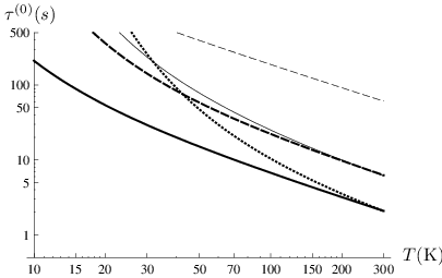
Let us next turn our attention to vibrational heating. To a good approximation, the vibrational eigenenergies of the deeply-bound states of a diatomic molecule are

E_{v}=h\omega_{\mathrm{e}}\bigl(v+{\textstyle\frac{1}{2}}\bigr),\quad v=0,1,\ldots

(70)

where $\omega_{\mathrm{e}}$ is the vibrational constant and $v$ is the vibrational quantum number. The corresponding eigenstates are

\langle q|v\rangle=\left(\frac{\alpha}{\pi}\right)^{1/4}\,\frac{1}{\sqrt{2^{v}v!}}\,H_{v}\bigl(\sqrt{\alpha}\,q\bigr)\mathrm{e}^{-\frac{1}{2}\alpha q^{2}},

(71)

where $q$ $\!=$ $R\!-\!R_{\mathrm{e}}$ , $R$ being the internuclear separation, $H_{n}$ are the Hermite polynomials and $\alpha=2\pi m\omega_{\mathrm{e}}/\hbar$ . Expanding the electric-dipole operator in a Taylor series about the equilibrium separation, $\hat{\bm{d}}$ $\!\approx$ $\!(\mu_{\mathrm{e}}+\mu^{\prime}_{\mathrm{e}}\hat{q})\hat{\bm{u}}$ , and recognizing that the first term cannot couple different vibrational states, we write the matrix elements for rovibrational transitions in the form

\langle v\,\Omega JM|\hat{\bm{d}}|v^{\prime}\,\Omega^{\prime}JM^{\prime}\rangle=\mu_{\mathrm{e}}^{\prime}\langle\Omega JM|\hat{\bm{u}}|\Omega^{\prime}J^{\prime}M^{\prime}\rangle\langle v|\hat{q}|v^{\prime}\rangle.

(72)

We see from this equation that the rovibrational transitions must satisfy the same rotational selection rules as already given above, and that to leading order in $q$ , the vibrational selection rule is $\Delta v$ $\!=$ $\!\pm 1$ . For transitions between $v^{\prime}=0$ and $v=1$ we have

\langle v=1|\hat{q}|v^{\prime}=0\rangle=\frac{1}{\sqrt{2\alpha}}=\sqrt{\frac{\hbar}{4\pi m\omega_{\mathrm{e}}}}\,.

(73)

We neglect the contribution of rotational energy to the transition frequency since it is typically smaller than the vibrational energy by two orders of magnitude. This means that we can simply add up the contributions of transitions (a)–(d) in calculating the transition dipole moments for OH and OD. Thus we obtain,

\sum_{k}|\bm{d}_{0k}|^{2}=\frac{\hbar\mu_{\mathrm{e}}^{\prime 2}}{4\pi m\omega_{\mathrm{e}}}\,f_{\mathrm{rot}}

(74)

where $f_{\mathrm{rot}}=1$ for the $\Sigma$ molecules, while for molecules with a ${}^{2}\Pi_{3/2}$ ground state,

f_{\mathrm{rot}}={\textstyle\frac{14}{15}}c_{+}^{2}(3/2)+{\textstyle\frac{2}{5}}c_{-}^{2}(3/2)+{\textstyle\frac{4}{15}}c_{+}^{2}(3/2)c_{-}^{2}(3/2).

(75)

		$\tau^{(0)}(\mathrm{s})$
Species	$\frac{\omega_{k0}}{2\pi}(\mathrm{THz})$	$T=293\mathrm{K}$	$T=77\mathrm{K}$
LiH	$\;42.1\;$	$\;25\;$	$\;6.5\!\times\!10^{9}\;$
NH	$\;98.4\;$	$\;310,\!000\;$	$\;1.3\!\times\!10^{25}\;$
OH	$\;112\;$	$\;9.8\!\times\!10^{6}\;$	$\;2.2\!\times\!10^{29}\;$
OD	$\;81.6\;$	$\;200,\!000\;$	$\;3.7\!\times\!10^{21}\;$
CaF	$\;18.4\;$	$4.7$	$23,\!000$
BaF	$\;14.1\;$	$\;1.8\;$	$\;1,\!300\;$
YbF	$\;15.2\;$	$\;4.1\;$	$\;4,\!700\;$
LiRb	$\;5.55\;$	$\;128\;$	$\;2,\!700\;$
NaRb	$\;3.21\;$	$\;1,\!400\;$	$\;13,\!000\;$
KRb	$\;2.26\;$	$\;120,\!000\;$	$\;850,\!000\;$
LiCs	$\;4.92\;$	$\;80\;$	$\;1,\!300\;$
NaCs	$\;2.94\;$	$\;580\;$	$\;4,\!900\;$
KCs	$\;1.98\;$	$\;12,\!000\;$	$\;74,\!000\;$
RbCs	$\;1.48\;$	$\;63,\!000\;$	$\;350,\!000\;$

Table 3: Lifetime against free-space vibrational heating out of the ground state for various polar molecules at

293\,\mathrm{K}

and

77\,\mathrm{K}

. For comparison with the results of [10], see [58].

The calculated lifetimes for free-space vibrational heating out of the ground state are given in Tab. 3 for $T=293\,\mathrm{K}$ and $T=77\,\mathrm{K}$ . These lifetimes are mainly determined by the vibrational transition frequencies. Since $\omega_{\mathrm{e}}$ $\!\propto$ $\!1/\sqrt{m}$ , the lightest molecules have the highest vibration frequencies, which lie above the 17 THz peak of the room temperature spectrum, whilst the heaviest molecules vibrate well below this frequency. The vibrational transition frequencies of CaF, BaF and YbF fall close to this maximum, and of the molecules considered these three also have the largest values of $\mu_{\mathrm{e}}^{\prime}$ . For both reasons, the ground-state lifetimes of these molecules are limited by vibrational heating to less than 5 s. For LiH and LiCs the vibrational heating is an order of magnitude slower, whilst it is exceedingly slow for all the other molecules. This slowness is mainly due to inefficient coupling with the thermal radiation which occurs both for the heavy molecules LiRb, NaRb, KRb, NaCs, KCs and RbCs whose vibration frequencies are too low and, even more strikingly, for the light molecules NH, OH and OD whose frequencies are too high.

Due to the large transition frequencies, the impact of lowering the environment temperature is even more striking for vibrational heating than in the rotational case. This is illustrated in Fig. 2 where the temperature-dependence of the lifetimes is displayed for the molecules LiH, CaF, BaF and YbF which are most strongly affected by vibrational heating.

The relative importance of rotational vs vibrational heating varies from molecule to molecule. Rotational heating dominates for the hydrides and for NaCs and KCs, while vibrational heating is dominant for the fluorides in the list, and for the other alkali dimers.

We have confined our attention to the rates for rotational and vibrational excitation out of the ground state. The calculation is very easily adapted to the excited states, remembering that then there will be both excitation processes to higher lying states, and de-excitation processes to lower lying ones. For the latter processes, $n(\omega_{k0})$ should be replaced with $n(\omega_{k0})+1$ to account for spontaneous emission. The calculations also need to be modified if applied electric or magnetic fields are present, so as to account for the Stark or Zeeman shifted transition frequencies, and any associated change in the transition dipole moments.

IV.2 Molecules near a surface

We turn now to the question of how proximity to a surface can affect the heating rate. Let us consider a molecule at distance $z_{\!A}$ from the surface of a homogeneous magneto-electric body of (relative) permittivity $\varepsilon(\omega)$ and (relative) permeability $\mu(\omega)$ . The body can be modelled by a semi-infinite half space provided it is close enough to the molecule and sufficiently smooth. The scattering part of the Green tensor is then given by

\mbox{{{{G}}}}^{(1)}(\bm{r},\bm{r},\omega)\\ =\frac{\mathrm{i}}{8\pi}\int_{0}^{\infty}\mathrm{d}q\,\frac{q}{\beta}\,e^{2i\beta z}\biggl[\biggl(r_{s}-\frac{\beta^{2}c^{2}}{\omega^{2}}\,r_{p}\biggr)(\bm{e}_{x}\bm{e}_{x}+\bm{e}_{y}\bm{e}_{y})\\ +2\,\frac{q^{2}c^{2}}{\omega^{2}}\,r_{p}\bm{e}_{z}\bm{e}_{z}\biggr]

(76)

where

r_{s}=\frac{\mu(\omega)\beta-\beta_{1}}{\mu(\omega)\beta+\beta_{1}}\,,\qquad r_{p}=\frac{\varepsilon(\omega)\beta-\beta_{1}}{\varepsilon(\omega)\beta+\beta_{1}}

(77)

are the reflection coefficients for $s$ - and $p$ -polarised waves,

\beta=\sqrt{\frac{\omega^{2}}{c^{2}}-q^{2}},\qquad\beta_{1}=\sqrt{\frac{\omega^{2}}{c^{2}}\,\varepsilon(\omega)\mu(\omega)-q^{2}}

(78)

( $\operatorname{Im}\beta$ , $\operatorname{Im}\beta_{1}$ $\!\geq$ $\!0$ ) denote the $z$ -component of the wave vector in free space ( $\beta$ ) and inside the half space ( $\beta_{1}$ ) and $q$ is its component parallel to the surface. For computational purposes, it is often convenient to express the Green tensor as an integral over $\beta$ ,

\mbox{{{{G}}}}^{(1)}(\bm{r},\bm{r},\omega)\\ =\frac{\mathrm{i}}{8\pi}\int_{0}^{\omega/c}\mathrm{d}\beta\,e^{2i\beta z}\biggl[\biggl(r_{s}-\frac{\beta^{2}c^{2}}{\omega^{2}}\,r_{p}\biggr)(\bm{e}_{x}\bm{e}_{x}+\bm{e}_{y}\bm{e}_{y})\\ +2\biggl(1-\frac{\beta^{2}c^{2}}{\omega^{2}}\biggr)r_{p}\bm{e}_{z}\bm{e}_{z}\biggr]\\ +\frac{1}{8\pi}\int_{0}^{\infty}\mathrm{d}b\,e^{-2bz}\biggl[\biggl(r_{s}+\frac{b^{2}c^{2}}{\omega^{2}}\,r_{p}\biggr)(\bm{e}_{x}\bm{e}_{x}+\bm{e}_{y}\bm{e}_{y})\\ +2\biggl(1+\frac{b^{2}c^{2}}{\omega^{2}}\biggr)r_{p}\bm{e}_{z}\bm{e}_{z}\biggr]

(79)

( $\beta$ $\!=$ $\!\mathrm{i}b$ ). Here, the first term represents the oscillating contributions due to travelling waves, while the second term contains the exponentially decaying contributions from evanescent waves.

Transition rates for a molecule near a half space can be obtained by substituting the scattering part of the Green tensor $\mbox{{{{G}}}}^{(1)}$ [as given by Eq. (76) or (79)] together with its free-space part [Eq. (40)] into Eq. (31). The ground-state heating rates then take the particularly simple form

	$\displaystyle\Gamma(\bm{r}_{\!A})$	$\displaystyle\!=$	$\displaystyle\!\Gamma^{(0)}+\Gamma^{(1)}(\bm{r}_{\!A})$		(80)
		$\displaystyle\!=$	$\displaystyle\!\Gamma^{(0)}\left[1+\frac{2\pi c}{\omega_{k0}}\operatorname{Im}\operatorname{tr}\mbox{{{{G}}}}^{(1)}(\bm{r}_{\!A},\bm{r}_{\!A},\omega_{k0})\right].$		(80)

In general, the integral appearing in Eq. (76) or (79) has to be evaluated numerically, but analytic results can be obtained for sufficiently small or large molecule–surface separations. The non-retarded limit applies to short distances, where $z|\sqrt{\varepsilon\mu}|\omega/c$ $\!\ll$ $\!1$ , while the retarded limit holds for long distances such that $z\omega/c$ $\!\gg$ $\!1$ . For the materials we consider in this paper, $|\sqrt{\varepsilon\mu}|$ takes on values between $65$ and $27,\!000$ for rotational transitions and between $4.5$ and $700$ for vibrational transitions, depending on the molecule and the material. Consequently, there is quite a large range of intermediate distances where neither limit applies.

In the non-retarded limit, the Green tensor (79) is dominated by the integral over evanescent waves, which effectively extends up to a wave vector $b$ $\!=$ $\!1/(2z)$ . Over most of this region, $\beta$ $\!\simeq$ $\!\beta_{1}$ $\!\simeq\mathrm{i}q$ , allowing us to use the approximations

r_{s}\simeq\frac{\mu(\omega)-1}{\mu(\omega)+1}\,,\qquad r_{p}\simeq\frac{\varepsilon(\omega)-1}{\varepsilon(\omega)+1}\,.

(81)

Performing the remaining integral and retaining only the leading order in $z\omega/c$ , one finds that in this non-retarded limit, the Green tensor is well approximated by [31]

\mbox{{{{G}}}}^{(1)}(\bm{r},\bm{r},\omega)\\ =\frac{c^{2}}{32\pi\omega^{2}z^{3}}\,\frac{\varepsilon(\omega)-1}{\varepsilon(\omega)+1}\,(\bm{e}_{x}\bm{e}_{x}+\bm{e}_{y}\bm{e}_{y}+2\bm{e}_{z}\bm{e}_{z}).

(82)

Note that by retaining only the leading order in $z\omega/c$ , the dependence on $r_{s}$ and thus also that on $\mu$ has vanished. In any case, $\mu$ is close to 1 even for the ferromagnetic metals at the typical frequencies of interest here (i.e. $\omega/2\pi>10\,\mathrm{GHz}$ ). On substituting Eq. (82) into Eq. (31), we obtain the approximate, near-field transition rate

\Gamma_{nk}(z_{\!A})=\Gamma_{nk}^{(0)}+\frac{|\bm{d}_{nk}|^{2}+|d_{nk,z}|^{2}}{8\pi\varepsilon_{0}\hbar z_{\!A}^{3}}\,\frac{\operatorname{Im}\varepsilon(\omega_{nk})}{|\varepsilon(\omega_{nk})+1|^{2}}\\ \times\{\Theta(\omega_{nk})[n(\omega_{nk})+1]-\Theta(\omega_{kn})n(\omega_{kn})\}.

(83)

In particular, the ground-state heating rates (80) are approximated by

\Gamma(z_{\!A})=\Gamma^{(0)}\biggl(1+\frac{z_{\mathrm{nr}}^{3}}{z_{\!A}^{3}}\biggr)

(84)

where

z_{\mathrm{nr}}=\frac{c}{\omega_{k0}}\,\sqrt[3]{\frac{\operatorname{Im}\varepsilon(\omega_{k0})}{2|\varepsilon(\omega_{k0})+1|^{2}}}

(85)

is a scaling length that applies to calculations in the non-retarded limit. For a metal with permittivity

\varepsilon(\omega)=1-\frac{\omega_{\mathrm{P}}^{2}}{\omega(\omega+\mathrm{i}\gamma)}

(86)

and provided that the transition frequency is sufficiently small, $\omega_{k0}\ll\gamma\leq\omega_{\mathrm{P}}$ , $z_{\mathrm{nr}}$ may be estimated by the simple relation

z_{\mathrm{nr}}=c\,\sqrt[3]{\frac{\gamma}{2\omega_{\mathrm{P}}^{2}\omega_{k0}^{2}}}\,.

(87)

The plasma frequency, $\omega_{\mathrm{P}}$ , and damping constant, $\gamma$ , are given for various conductors in Tab. 4.

We stress that Eq. (84) applies only in the non-retarded limit, and that the distance $z_{\mathrm{nr}}$ typically lies well outside this limit. We define a second relevant length scale, $z_{\mathrm{c}}$ , the characteristic distance at which the surface-induced rate becomes equal to the free-space rate. This does not coincide with $z_{\mathrm{nr}}$ , because the non-retarded limit is not valid at this distance. We have calculated $z_{\mathrm{c}}$ by numerical integration of Eqs. (79) and (80) and we present the results for molecules near a gold surface in Tab. 5, and for a range of other conductors in App. B. The table also gives the corresponding values of $z_{\mathrm{nr}}$ , which are typically $2$ – $5$ times smaller.

Since Eq. (84) does not apply at length scales in the vicinity of the critical distance, we searched for an alternative formula by fitting to the numerical results obtained from the integration of Eqs. (79) and (80) at distances $z$ $\!\leq$ $\!z_{\mathrm{c}}$ . We find that for the molecules and surface materials studied, the heating rates throughout this range are well approximated by the empirical formula

\Gamma(z_{\!A})=\Gamma^{(0)}\biggl(1+\frac{z_{\mathrm{c}}^{2}}{z_{\!A}^{2}}+\frac{z_{\mathrm{nr}}^{3}}{z_{\!A}^{3}}\biggr).

(88)

Furthermore, a fit to the set of critical distances for rotational heating given in App. B, suggests the approximate formula

z_{\mathrm{c}}\simeq\frac{3c}{4}\,\sqrt[4]{\frac{\gamma}{2\omega_{\mathrm{P}}^{2}\omega_{k0}^{3}}}\,.

(89)

This empirical formula was found to be accurate to within 1% for all the surfaces and molecules considered, except in cases where the critical distances are particularly small (the hydrides and KCs), where deviations between 1% and 10% are more typical. The same formula does not accurately predict the critical distances for vibrational heating, but these are of less importance due to their very small values. We stress again that Eq. (88) is only empirical as the $z_{\!A}^{-2}$ term has no physical interpretation.

Material	$\omega_{\mathrm{P}}(\mbox{rad/s})$	$\gamma(\mbox{rad/s})$	$\omega_{\mathrm{P}}^{2}/\gamma(\mbox{rad/s})$
Au	$\;1.37\!\times\!10^{16}\;$	$\;4.12\!\times\!10^{13}\;$	$\;4.53\!\times\!10^{18}\;$
Al	$\;2.25\!\times\!10^{16}\;$	$\;1.22\!\times\!10^{14}\;$	$\;4.15\!\times\!10^{18}\;$
Pd	$\;8.36\!\times\!10^{15}\;$	$\;2.16\!\times\!10^{13}\;$	$\;3.24\!\times\!10^{18}\;$
Ag	$\;5.77\!\times\!10^{15}\;$	$\;1.15\!\times\!10^{13}\;$	$\;2.89\!\times\!10^{18}\;$
Cu	$\;1.12\!\times\!10^{16}\;$	$\;4.41\!\times\!10^{13}\;$	$\;2.87\!\times\!10^{18}\;$
Mo	$\;1.14\!\times\!10^{16}\;$	$\;7.86\!\times\!10^{13}\;$	$\;1.65\!\times\!10^{18}\;$
Fe	$\;6.23\!\times\!10^{15}\;$	$\;2.79\!\times\!10^{13}\;$	$\;1.39\!\times\!10^{18}\;$
Co	$\;1.18\!\times\!10^{16}\;$	$\;1.07\!\times\!10^{14}\;$	$\;1.29\!\times\!10^{18}\;$
W	$\;9.72\!\times\!10^{15}\;$	$\;8.53\!\times\!10^{13}\;$	$\;1.11\!\times\!10^{18}\;$
Ni	$\;7.44\!\times\!10^{15}\;$	$\;6.53\!\times\!10^{13}\;$	$\;8.49\!\times\!10^{17}\;$
Pt	$\;7.75\!\times\!10^{15}\;$	$\;1.04\!\times\!10^{14}\;$	$\;5.75\!\times\!10^{17}\;$
ITO	$\;3.33\!\times\!10^{15}\;$	$\;1.68\!\times\!10^{14}\;$	$\;6.63\!\times\!10^{16}\;$

Table 4: Drude parameters for various conductors. Values are taken from Ref. [62], with the exception of those for ITO (indium tin oxide) [63]. The list is in order of decreasing

\omega_{\mathrm{P}}^{2}/\gamma

, which corresponds to increasing surface heating rate.

	Rotational		Vibrational
Species	$z_{\mathrm{nr}}(\mu\mathrm{m})$	$z_{\mathrm{c}}(\mu\mathrm{m})$	$z_{\mathrm{nr}}(\mu\mathrm{m})$	$z_{\mathrm{c}}(\mu\mathrm{m})$
LiH	$0.73$	$1.9$	$0.035$	$0.071$
NH	$0.42$	$1.0$	$0.020$	$0.042$
OH			$0.018$	$0.0039$
(a)	$0.23$	$0.50$
(b)	$0.17$	$0.36$
(c)	$0.13$	$0.27$
(d)	$0.10$	$0.20$
OD			$0.022$	$0.0048$
(a)	$0.34$	$0.78$
(b)	$0.17$	$0.35$
(c)	$0.15$	$0.30$
(d)	$0.12$	$0.24$
CaF	$5.5$	$19$	$0.061$	$0.12$
BaF	$7.8$	$27$	$0.072$	$0.14$
YbF	$7.1$	$25$	$0.069$	$0.14$
LiRb	$7.6$	$26$	$0.13$	$0.27$
NaRb	$17$	$64$	$0.19$	$0.41$
KRb	$24$	$98$	$0.24$	$0.54$
LiCs	$8.2$	$29$	$0.15$	$0.30$
NaCs	$3.9$	$13$	$0.21$	$0.44$
KCs	$1.3$	$3.6$	$0.27$	$0.60$
RbCs	$42$	$180$	$0.33$	$0.75$

Table 5: Non-retarded length scales and critical distances for surface enhancement of rotational and vibrational heating rates near a gold surface.

The critical distances given in Tab. 5 show that the surface does not generate any significant heating when the molecules are more than a few hundred $\mu\mathrm{m}$ away. However, if the molecules are held a few $\mu\mathrm{m}$ from a surface, as they might be on a molecule chip, there is a substantial increase in the rotational heating for all the molecules considered, apart from the hydrides. Even in cases where the free-space rate is small, the enhanced rate can be very large because of the rapid inverse-power scaling. For example, in free space, the rotational heating time of CaF, $3400\,\mathrm{s}$ , is enormous compared with the vibrational lifetime of $4.7\,\mathrm{s}$ . However, at a distance of $1\,\mu\mathrm{m}$ from a room temperature gold surface the lifetime for rotational excitation drops to about 8 s and at smaller distances the rotational heating rate dominates over the vibrational rate. For the hydrides, the high rotational frequency that gives them rapid free-space heating also makes them relatively insensitive to the proximity of the surface except at sub-micron distances.

Figure 3(a) shows the critical distances for rotational heating of various molecules near a range of surfaces. It is seen that their frequency scaling follows quite nicely the $\omega^{-3/4}$ dependence given by Eq. (89), which is indicated by the solid line. This trend continues in Fig. 3(b), which shows the critical distances for vibrational heating. These are, of course, smaller because the vibrational frequencies are higher.

Equation (87) shows that the short-range heating depends on the surface material through the factor $\omega_{\mathrm{P}}^{2}/\gamma$ . A low value of this ratio leads to a large critical distance and hence to more surface-induced heating. The values are displayed in the last column of Tab. 4 for various metals in order of decreasing $\omega_{\mathrm{P}}^{2}/\gamma$ . In this list, gold is the metal of choice when trying to minimise surface-induced heating of the molecules, as also indicated by the circles in Fig. 3. At the opposite extreme lies indium tin oxide (ITO), which we include here because of its attractive combination of conductivity and optical transparency. It has a low plasma frequency and a high damping rate $\gamma$ and so generates stronger heating, as shown by the triangles in Fig. 3. The values for other metals generally obey the $\omega_{\mathrm{P}}^{2}/\gamma$ scaling, though there are some exceptions where values of $\omega_{\mathrm{P}}^{2}/\gamma$ are very similar.

As indicated by Eq. (85), the surface-induced heating will be particularly large in cases where $|\varepsilon|$ is not large, but $\varepsilon$ has a significant imaginary part. This never happens for a conductor, but can occur for dielectric media that happen to be strong absorbers at the relevant frequency. As an example, consider borosilicate glass which has $\varepsilon$ $\!=$ $\!6.2+0.21\mathrm{i}$ for frequencies in the tens of GHz range [64]. The critical distance for rotational heating of CaF near such a surface is about $620\,\mu\mathrm{m}$ , very much larger than for a metallic surface. The timescale for rotational heating, which is $3400\,\mathrm{s}$ in free space, is thus reduced to just $0.14\,\mathrm{s}$ when this molecule is $10\,\mu\mathrm{m}$ from such a glass surface.

Next, we turn to the retarded limit, where $z\omega/c$ $\!\gg$ $\!1$ , so the integrand in Eq. (79) is rapidly oscillating or decaying over most parts of the integration regime. The main contribution to the integral (79) comes from the region around the stationary-phase point $q$ $\!=$ $\!0$ , so that we may approximate

r_{s}\simeq-r_{p}\simeq\frac{\sqrt{\mu(\omega)}-\sqrt{\varepsilon(\omega)}}{\sqrt{\mu(\omega)}+\sqrt{\varepsilon(\omega)}}\,.

(90)

The integral can then be performed, and upon retaining the leading order in $c/(z\omega)$ , one finds that the Green tensor in the retarded limit reads

\mbox{{{{G}}}}^{(1)}(\bm{r},\bm{r},\omega)=\frac{e^{2\mathrm{i}z\omega/c}}{8\pi z}\,\frac{\sqrt{\mu(\omega)}-\sqrt{\varepsilon(\omega)}}{\sqrt{\mu(\omega)}+\sqrt{\varepsilon(\omega)}}\\ \times(\bm{e}_{x}\bm{e}_{x}+\bm{e}_{y}\bm{e}_{y}).

(91)

Consequently, the transition rates (31) are given by

\Gamma_{nk}(z_{\!A})=\Gamma_{nk}^{(0)}+\frac{\omega_{nk}^{2}\bigl(|d_{nk,x}|^{2}\!+\!|d_{nk,y}|^{2}\bigr)}{4\pi\varepsilon_{0}\hbar c^{2}z_{\!A}}\\ \times\operatorname{Im}\Biggl(\frac{\sqrt{\mu(\omega_{nk})}-\sqrt{\varepsilon(\omega_{nk})}}{\sqrt{\mu(\omega_{nk})}+\sqrt{\varepsilon(\omega_{nk})}}\,e^{2\mathrm{i}z_{\!A}\omega_{nk}/c}\Biggr)\\ \times\{\Theta(\omega_{nk})[n(\omega_{nk})+1]-\Theta(\omega_{kn})n(\omega_{kn})\};

(92)

for a good conductor, $|\varepsilon|$ $\!\gg$ $\!|\mu|$ , they further simplify to

\Gamma_{nk}(z_{\!A})=\Gamma_{nk}^{(0)}-\frac{\omega_{nk}^{2}\bigl(|d_{nk,x}|^{2}\!+\!|d_{nk,y}|^{2}\bigr)}{4\pi\varepsilon_{0}\hbar c^{2}z_{\!A}}\sin\biggl(\frac{2z_{\!A}\omega_{nk}}{c}\biggr)\\ \times\{\Theta(\omega_{nk})[n(\omega_{nk})+1]-\Theta(\omega_{kn})n(\omega_{kn})\}.

(93)

In particular, the ground-state heating rates (80) are given by

$\displaystyle\Gamma(z_{\!A})$	$\displaystyle\!=$	$\displaystyle\!\Gamma^{(0)}\Biggl[1+\frac{c}{2z_{\!A}\omega_{k0}}\,$	(94)
		$\displaystyle\!\times\operatorname{Im}\Biggl(\frac{\sqrt{\mu(\omega_{k0})}-\sqrt{\varepsilon(\omega_{k0})}}{\sqrt{\mu(\omega_{k0})}+\sqrt{\varepsilon(\omega_{k0})}}\,e^{2\mathrm{i}z_{\!A}\omega_{k0}/c}\Biggr)\Biggr]$
	$\displaystyle\!\simeq$	$\displaystyle\!\Gamma^{(0)}\biggl[1-\frac{c}{2z_{\!A}\omega_{k0}}\,\sin\biggl(\frac{2z_{\!A}\omega_{nk}}{c}\biggr)\biggr]\,.$

Thus, the surface-induced modification of the heating rates in the retarded limit is an oscillating function of distance, where the amplitude of the oscillation follows a $z_{\!A}^{-1}$ power law. In particular, the heating rates approach their free-space values in the limit $z_{\!A}$ $\!\to$ $\!\infty$ .

In order to see the entire distance dependence of the heating rate it is necessary to calculate the rates as given by Eq. (79) and (80) numerically. The results are displayed in Fig. 4 where we show the total heating rates as a function of distance for OH, LiH, CaF and NaCs molecules at distances in the range $1-500\,\mu\mathrm{m}$ from a gold surface. In all cases, the vibrational heating rate is dotted, the rotational rate is dashed and the total rate is a solid line. For OH the heating is entirely dominated by the rotational transitions over the whole of this distance range, and the vibrational contribution does not even appear in the plot. The heating rate is modulated with a period of $60\,\mu\mathrm{m}$ just as expected in the retarded limit [Eq. (94)]. The heating rate is not greatly altered from its free space value, even at the shortest distance considered. For LiH, the heating is again dominated by the rotational transitions. The far-field oscillations modulate the rate and we see roughly one cycle with a period of $338\,\mu\mathrm{m}$ . The heating rate rises sharply inside the critical distance for rotational excitation, which is $1.9\,\mu\mathrm{m}$ , whereas the vibrational contribution, having a much shorter critical distance, remains essentially constant down to $1\,\mu\mathrm{m}$ . For CaF, the heating is dominated by vibrational excitation at $18.4\,\mathrm{THz}$ , corresponding to an oscillation period in the far field of $8\,\mu\mathrm{m}$ , which can clearly be seen. Inside the $19\,\mu\mathrm{m}$ critical distance for rotational heating, we see a dramatic increase in the rotational contribution to the rate, such that the two contributions are roughly equal at a distance of $1\,\mu\mathrm{m}$ from the surface. For NaCs, the two contributions are roughly equal in the far field and both are rather small. The $3\,\mathrm{THz}$ vibrational heating exhibits the expected far-field oscillations, whilst the rotational heating is at too low a frequency to show oscillations over this range. Inside the $13\mu\mathrm{m}$ critical distance, the rotational heating increases rapidly, becoming a thousand times faster at a distance of $1\,\mu\mathrm{m}$ .

In Fig. 5, we show once again the heating rate for NaCs as a function of distance from a gold surface (solid line). This figure also shows for comparison the heating rates near iron and ITO surfaces. At distances large enough for the retarded limit to apply, the heating rate given by Eq. (94) is independent of the particular metallic surface since these are all good conductors at the relevant excitation frequencies. At short range however, where the near-field limit of Eq. (84) applies, the heating rate becomes proportional to $\gamma/\omega_{\mathrm{P}}^{2}$ . As shown in Tab. 4, this ratio differs widely between these materials and is a hundred times larger for ITO than for gold. For this reason, the ITO surface produces a larger heating rate at short distance and exhibits a longer critical distance than gold, as seen in Fig. 5.

So far, we have discussed surface-enhanced heating in the presence of metallic and dielectric surfaces. It is also interesting to consider the heating rate for molecules in the vicinity of meta-materials, since these offer tunable magneto-electric properties [65, 66], and can even be left-handed [67]. A left-handed medium is realized when the real parts of both $\varepsilon$ and $\mu$ are simultaneously negative, leading to a negative index of refraction and a number of counterintuitive effects associated with the propagation of the electromagnetic field inside such a medium [67]. Since the surface-enhanced heating rate of a single interface depends solely on the reflected electromagnetic field, one would expect it to be insensitive to left-handedness. For weakly absorbing media, the oscillations seen in the retarded limit are small when the signs of $\operatorname{Re}\varepsilon$ and $\operatorname{Re}\mu$ are both positive or both negative. In the case where $\operatorname{Re}\varepsilon$ $\!=$ $\!\operatorname{Re}\mu$ , and the imaginary parts are small, there are no oscillations at all since $r_{s}$ and $r_{p}$ are then very close to zero. The amplitude of the oscillations is greatest when these reflection coefficients have their maximum values of 1. As we have already seen, this occurs for metals because $|\varepsilon|$ is much larger than $|\mu|$ . In the context of meta-materials, reflection coefficients close to unity are obtained for any weakly absorbing medium where $\operatorname{Re}\varepsilon$ and $\operatorname{Re}\mu$ have opposite signs. Note that this result is insensitive to the magnitudes of $\operatorname{Re}\varepsilon,\operatorname{Re}\mu$ , which neither need to be equal nor particularly large; they need only be of opposite sign and considerably larger than the imaginary parts. A meta-material engineered with these properties would produce large oscillations in the heating rate with a phase determined by the chosen values of $\operatorname{Re}\varepsilon,\operatorname{Re}\mu$ .

Figure 6 shows the heating rate of a LiH molecule near fictitious weakly absorbing meta-materials with $\operatorname{Re}\varepsilon$ $\!=$ $\!\pm\operatorname{Re}\mu$ . We see that the left-handed material ( $\operatorname{Re}\varepsilon$ , $\operatorname{Re}\mu$ $\!<$ $\!0$ ) gives rise to exactly the same heating rate as a comparable ordinary material with $\operatorname{Re}\varepsilon$ , $\operatorname{Re}\mu$ $\!>$ $\!0$ (the two curves cannot be distinguished on the plot), and that the oscillations are suppressed. On the other hand, media with $\operatorname{Re}\varepsilon$ $\!=$ $-\operatorname{Re}\mu$ result in large oscillations of the heating rate in the long-distance regime, with a phase that depends on the material properties.

IV.3 Surfaces of finite thickness

The results of the previous section have shown that metallic surfaces can considerably enhance surface-induced heating. In the context of chips, metal surfaces are often unavoidable since they are used in current- or charge-carrying structures. One possible strategy to reduce the associated molecular heating is to reduce the thickness of the metal substrates. For a slab of finite thickness $d$ , coated onto an infinitely thick substrate of permittivity $\varepsilon_{\mathrm{s}}$ $\!=$ $\!\varepsilon_{\mathrm{s}}(\omega)$ and permeability $\mu_{\mathrm{s}}$ $\!=$ $\!\mu_{\mathrm{s}}(\omega)$ , the surface-induced heating rate is still given by Eq. (80) together with Eq. (79), but the reflection coefficients are now given by

		$\displaystyle r_{s}=\frac{\mu^{2}\beta\beta_{\mathrm{s}}-\mu_{\mathrm{s}}\beta_{1}^{2}+\mathrm{i}\mu\beta_{1}[\mu_{\mathrm{s}}\beta-\beta_{\mathrm{s}}]\cot(\beta_{1}d)}{\mu^{2}\beta\beta_{\mathrm{s}}+\mu_{\mathrm{s}}\beta_{1}^{2}+\mathrm{i}\mu\beta_{1}[\mu_{\mathrm{s}}\beta+\beta_{\mathrm{s}}]\cot(\beta_{1}d)}\,,$		(95)
		$\displaystyle r_{p}=\frac{\varepsilon^{2}\beta\beta_{\mathrm{s}}-\varepsilon_{\mathrm{s}}\beta_{1}^{2}+\mathrm{i}\varepsilon\beta_{1}[\varepsilon_{\mathrm{s}}\beta-\beta_{\mathrm{s}}]\cot(\beta_{1}d)}{\varepsilon^{2}\beta\beta_{\mathrm{s}}+\varepsilon_{\mathrm{s}}\beta_{1}^{2}+\mathrm{i}\varepsilon\beta_{1}[\varepsilon_{\mathrm{s}}\beta+\beta_{\mathrm{s}}]\cot(\beta_{1}d)}$		(96)

where

\beta_{\mathrm{s}}=\sqrt{\frac{\omega^{2}}{c^{2}}\,\varepsilon_{\mathrm{s}}(\omega)\mu_{\mathrm{s}}(\omega)-q^{2}}

(97)

( $\operatorname{Im}\beta_{\mathrm{s}}$ $\!\geq$ $\!0$ ).

Let us first consider the influence of the metal surface alone by letting $\varepsilon_{\mathrm{s}}=\mu_{\mathrm{s}}=1$ . In the non-retarded limit, the reflection coefficients may then be approximated by

	$\displaystyle r_{s}$	$\displaystyle\!\simeq$	$\displaystyle\!\frac{\mu^{2}-1}{\mu^{2}+1+2\mu\coth(qd)}\,,\qquad$		(98)
	$\displaystyle r_{p}$	$\displaystyle\!\simeq$	$\displaystyle\!\frac{\varepsilon^{2}-1}{\varepsilon^{2}+1+2\varepsilon\coth(qd)}$		(99)

[recall the discussion above Eq. (81)]. Since $q$ $\!\lesssim$ $\!1/(2z_{\!A})$ , the short-range heating rate will be identical to that of an infinitely thick plate provided $d$ $\!\gg$ $\!z_{\!A}$ , since in this limit the above reflection coefficients reduce to those given in Eqs. (77). On the other hand, the reflection coefficients, and hence also the heating rate, must become very small when $d|\varepsilon|$ $\!\ll$ $\!z_{\!A}$ . We note immediately that, for molecule–surface separations of interest, a conducting surface needs to be unfeasibly thin for this limit to be reached, because of the enormously large values of $|\varepsilon|$ for a conductor. The behaviour between the two limits has to be determined from a numerical analysis.

In the retarded limit, one may approximate

r_{s}\simeq-r_{p}\simeq\frac{\varepsilon-\mu}{\varepsilon+\mu+2\mathrm{i}\sqrt{\varepsilon\mu}\,\cot\bigl(\sqrt{\varepsilon\mu}\,\omega d/c\bigr)}

(100)

so for a good conductor, $|\varepsilon|$ $\!\gg$ $\!|\mu|$ , the reflection coefficients and the heating rate become independent of the plate thickness at long range.

In Fig. 7, we display the surface-induced heating rate of a NaCs molecule near ITO plates of various thicknesses as a function of molecule–plate separation.

At large separations, the heating rates are independent of the thickness, as predicted from Eq. (100). Over the entire range of distances calculated, the ITO plate of thickness $\!10\mu\mathrm{m}$ gives the same result as a plate of infinite thickness. Reducing the thickness below this value increases the heating rates at short distances, contrary to the expectation of reduced rates at short range anticipated from Eqs. (98) and (99). A reduction of the short-range heating rates below the values observed for thick plates is eventually found but only once the coating is unfeasibly thin. Thus our calculations show that the heating at short-range cannot be reduced by reducing the material thickness. To understand the increase of the heating rate with decreasing thickness, note that in the non-retarded limit the heating is mainly due to the coupling of the molecule with the surface plasmons at the front face of the plate. As the thickness decreases, these couple to the plasmons at the back face of the plate, leading to mutual enhancement and thus to an increase of the heating rate [68]. To include the borosilicate glass substrate we took $\varepsilon_{\mathrm{s}}(\omega_{k0})$ $\!=$ $\!6.2+0.21\mathrm{i}$ for the rotational transitions [64] and $\varepsilon_{\mathrm{s}}(\omega_{k0})$ $\!=$ $\!6.4+0.74\mathrm{i}$ for the vibrational ones [69]. We find identical results whether or not this substrate is included, except for the thinnest coating, $d=0.01\,\mu$ m, where we find that the presence of the substrate slightly reduces the heating rate, as shown by the thin solid line in the figure.

V Summary and conclusions

Using macroscopic QED, we have calculated the internal dynamics of a molecule placed within an arbitrary environment of magneto-electric bodies of uniform temperature. The internal time evolution is governed by the molecular transition frequencies and transition rates which depend on position and temperature. The dependence on temperature is due to the thermal photon number and can be completely understood from considering the free-space case, while the position-dependence, which enters via the classical Green tensor for the electromagnetic field in the environment, can be derived from the behaviour at zero temperature.

We have used the general formulae to study the ground-state heating rates of several polar molecules of current experimental interest, as a function of the distance from various surfaces. We have given a simple approximate formula that can be used to estimate the heating rates for any other molecules at any distance from any surface of interest. For light molecules, particularly the hydrides, rotational heating dominates and limits the free-space lifetime of the ground state to a few seconds when the environment is at room temperature. For the metal fluorides we studied, vibrational heating dominates and again the room temperature free-space lifetime of the ground state is of the order of a few seconds. When the molecules approach a metallic surface, the heating rate can be greatly enhanced. This is particularly true for the rotational transitions where the critical distance at which the surface dominates the free-space rate is typically in the $1-100\,\mu\mathrm{m}$ range. For the hydrides, the free-space heating rate is large because the rotational frequencies are large, but this same fact also means that the critical distance for surface-induced heating is rather small. Therefore, these molecules could be trapped up to a few microns from a surface with little change in the heating rate. The effect of the surface on rotational heating is very much stronger for the heavier molecules, but since the rate in free-space is typically very small for these molecules, they too have lifetimes of a second or more at distances up to 1 $\mu$ m from the surface.

We have shown that, at long range, the heating rates become insensitive to the particular surface properties, while at short-range the heating is faster for smaller values of the parameter $\omega_{\mathrm{P}}^{2}/\gamma$ . Of the metals considered, gold induces the lowest heating rate. We have also shown that decreasing the thickness of the surface tends to increase the heating rate, particularly at short distances. Dielectric materials that are good absorbers at the relevant frequency result in large critical distances and hence very large heating rates at short range.

In the context of molecule chips, where confinement of molecules a few microns from the chip surface is envisaged, our work shows that surface-induced heating should be considered carefully when selecting appropriate molecules and surfaces, but that confinement for several seconds in single quantum-states is quite feasible even when the surface is at room temperature. In all cases, lowering the environment temperature will allow for even longer lifetimes. For approach distances smaller than $1\,\mu\mathrm{m}$ , surface-induced heating becomes rapidly problematic, and cooling to cryogenic temperatures may be required.

Acknowledgements.

This work was supported by the Alexander von Humboldt Foundation, the Royal Society, and the UK Engineering and Physical Sciences Research Council. The research leading to these results has received funding from the European Community’s Seventh Framework Programme FP7/2007-2013 under grant agreement 216774. S.Y.B is grateful to W.L. Barnes, S. Franzen, C. Henkel, J. Kirkpatrick, G.J. McPhee, B.E. Sernelius and M.S. Tomaš for dicussions.

Appendix A Markov approximation

Substituting the formal solution

\hat{\bm{f}}_{\lambda}(\bm{r},\omega,t)=\mathrm{e}^{-\mathrm{i}\omega t}\hat{\bm{f}}_{\lambda}(\bm{r},\omega)\\ +\frac{\mathrm{i}}{\hbar}\sum_{m,n}\int_{0}^{t}\mathrm{d}\tau\,\mathrm{e}^{-\mathrm{i}\omega(t-\tau)}\bm{d}_{mn}\!\cdot\!\mbox{{{{G}}}}_{\lambda}^{\ast}(\bm{r}_{\!A},\bm{r},\omega)\hat{A}_{mn}(\tau)

(101)

to Eq. (27) into Eq. (26) and using the integral relation (13), one obtains

\dot{\hat{A}}_{mn}(t)=\mathrm{i}\omega_{mn}\hat{A}_{mn}(t)+\frac{\mathrm{i}}{\hbar}\sum_{k}\int_{0}^{\infty}\mathrm{d}\omega\\ \times\biggl\{\mathrm{e}^{-\mathrm{i}\omega t}\bigl[\bm{d}_{nk}\hat{A}_{mk}(t)-\bm{d}_{km}\hat{A}_{kn}(t)\bigr]\!\cdot\!\underline{\hat{\bm{E}}}(\bm{r}_{\!A},\omega)\\ +\mathrm{e}^{\mathrm{i}\omega t}\underline{\hat{\bm{E}}}{}^{\dagger}(\bm{r}_{\!A},\omega)\!\cdot\!\bigl[\bm{d}_{nk}\hat{A}_{mk}(t)-\bm{d}_{km}\hat{A}_{kn}(t)\bigr]\biggr\}\\ +\hat{Z}_{mn}(t)

(102)

with

\hat{Z}_{mn}(t)=-\frac{\mu_{0}}{\hbar\pi}\sum_{k,l,j}\int_{0}^{\infty}\mathrm{d}\omega\omega^{2}\int_{0}^{t}\mathrm{d}\tau\\ \times\bigl\{\bigl[\mathrm{e}^{-\mathrm{i}\omega(t-\tau)}\hat{A}_{mk}(t)\hat{A}_{lj}(\tau)-\mathrm{e}^{\mathrm{i}\omega(t-\tau)}\hat{A}_{lj}(\tau)\hat{A}_{mk}(t)\bigr]\\ \times\bm{d}_{nk}\!\cdot\!\operatorname{Im}\mbox{{{{G}}}}(\bm{r}_{\!A},\bm{r}_{\!A},\omega)\!\cdot\!\bm{d}_{lj}\\ -\bigl[\mathrm{e}^{-\mathrm{i}\omega(t-\tau)}\hat{A}_{kn}(t)\hat{A}_{lj}(\tau)-\mathrm{e}^{\mathrm{i}\omega(t-\tau)}\hat{A}_{lj}(\tau)\hat{A}_{nk}(t)\bigr]\\ \times\bm{d}_{km}\!\cdot\!\operatorname{Im}\mbox{{{{G}}}}(\bm{r}_{\!A},\bm{r}_{\!A},\omega)\!\cdot\!\bm{d}_{lj}\bigr\}

(103)

denoting the zero-point contribution to the internal molecular dynamics. This differential equation can be solved iteratively by substituting the self-consistent solution

\hat{A}_{mn}(t)=\mathrm{e}^{\mathrm{i}\tilde{\omega}_{mn}t}\hat{A}_{mn}(0)\\ +\frac{\mathrm{i}}{\hbar}\sum_{k}\int_{0}^{\infty}\mathrm{d}\omega\int_{0}^{t}\mathrm{d}\tau\,\mathrm{e}^{\mathrm{i}\tilde{\omega}_{mn}(t-\tau)}\\ \times\biggl\{\mathrm{e}^{-\mathrm{i}\omega\tau}\bigl[\bm{d}_{nk}\hat{A}_{mk}(\tau)-\bm{d}_{km}\hat{A}_{kn}(\tau)\bigr]\!\cdot\!\underline{\hat{\bm{E}}}(\bm{r}_{\!A},\omega)\\ +\mathrm{e}^{\mathrm{i}\omega\tau}\underline{\hat{\bm{E}}}{}^{\dagger}(\bm{r}_{\!A},\omega)\!\cdot\!\bigl[\bm{d}_{nk}\hat{A}_{mk}(\tau)-\bm{d}_{km}\hat{A}_{kn}(\tau)\bigr]\biggr\}

(104)

to the truncated Eq. (102) without $\hat{Z}_{mn}(t)$ back into Eq. (102), where at this level of approximation, the operator ordering in Eq. (104) may be chosen arbitrarily. Taking expectation values according to Eqs. (15)–(18), one arrives at

\bigl\langle\dot{\hat{A}}_{mn}(t)\bigl\rangle=\mathrm{i}\omega_{mn}\bigl\langle\hat{A}_{mn}(t)\bigl\rangle+\bigl\langle\hat{T}_{mn}(t)\bigl\rangle+\bigl\langle\hat{Z}_{mn}(t)\bigl\rangle

(105)

where

\bigl\langle\hat{T}_{mn}(t)\bigl\rangle\\ =-\frac{\mu_{0}}{\hbar\pi}\sum_{k,l}\int_{0}^{\infty}\mathrm{d}\omega\,\omega^{2}n(\omega)\int_{0}^{t}\mathrm{d}\tau\bigl[\mathrm{e}^{-\mathrm{i}\omega(t-\tau)}+\mathrm{e}^{\mathrm{i}\omega(t-\tau)}\bigr]\\ \times\Bigl\{\mathrm{e}^{\mathrm{i}\tilde{\omega}_{mk}(t-\tau)}\bigl[\bigl\langle\hat{A}_{ml}(\tau)\bigl\rangle\bm{d}_{nk}\!\cdot\!\operatorname{Im}\mbox{{{{G}}}}(\bm{r}_{\!A},\bm{r}_{\!A},\omega)\!\cdot\!\bm{d}_{kl}\\ -\bigl\langle\hat{A}_{lk}(\tau)\bigl\rangle\bm{d}_{nk}\!\cdot\!\operatorname{Im}\mbox{{{{G}}}}(\bm{r}_{\!A},\bm{r}_{\!A},\omega)\!\cdot\!\bm{d}_{lm}\bigr]\\ -\mathrm{e}^{\mathrm{i}\tilde{\omega}_{kn}(t-\tau)}\bigl[\bigl\langle\hat{A}_{kl}(\tau)\bigl\rangle\bm{d}_{km}\!\cdot\!\operatorname{Im}\mbox{{{{G}}}}(\bm{r}_{\!A},\bm{r}_{\!A},\omega)\!\cdot\!\bm{d}_{nl}\\ -\bigl\langle\hat{A}_{ln}(\tau)\bigl\rangle\bm{d}_{km}\!\cdot\!\operatorname{Im}\mbox{{{{G}}}}(\bm{r}_{\!A},\bm{r}_{\!A},\omega)\!\cdot\!\bm{d}_{lk}\bigr]\Bigr\}

(106)

denotes the thermal contribution to the internal molecular dynamics. For weak molecule–field coupling, the contributions $\bigl\langle\hat{T}_{mn}(t)\bigl\rangle$ and $\bigl\langle\hat{Z}_{mn}(t)\bigl\rangle$ may be evaluated by means of the Markov approximation, i.e. by letting $\bigl\langle\hat{A}_{mn}(\tau)\bigr\rangle$ $\!\simeq$ $\!\mathrm{e}^{-\mathrm{i}\tilde{\omega}_{mn}(t-\tau)}\bigl\langle\hat{A}_{mn}(t)\bigr\rangle$ and evaluating the remaining time integrals according to

\int_{0}^{t}\mathrm{d}\tau\,\mathrm{e}^{-\mathrm{i}(\omega-\tilde{\omega}_{mn})(t-\tau)}\\ \simeq\pi\delta(\omega-\tilde{\omega}_{mn})+\mathrm{i}\mathcal{P}\,\frac{1}{\tilde{\omega}_{mn}-\omega}\,.

(107)

Assuming the system to be non-degenerate, so that off-diagonal molecular density matrix decouple from each other as well as from the diagonal ones, we arrive at Eqs. (28) and (29), together with Eqs. (30)–(38).

Appendix B Critical distances

We have calculated the critical distances for surface-induced enhancement of ground-state heating rates for various combinations of molecules and materials on the basis of the data given in Tabs. 1 and 4. The results are summarised in Tab. 6.

	rotational											vibrational
Spe.	Al	Pd	Ag	Cu	Mo	Fe	Co	W	Ni	Pt	ITO	Al	Pd	Ag	Cu	Mo	Fe	Co	W	Ni	Pt	ITO
LiH	$1.9$	$2.0$	$2.0$	$2.1$	$2.4$	$2.5$	$2.6$	$2.7$	$2.8$	$3.1$	$5.4$	$.044$	$.038$	$.039$	$.042$	$.053$	$.051$	$.060$	$.060$	$.064$	$.075$	$.16$
NH	$1.0$	$1.0$	$1.0$	$1.1$	$1.3$	$1.3$	$1.4$	$1.4$	$1.5$	$1.7$	$2.9$	$.021$	$.022$	$.023$	$.023$	$.028$	$.029$	$.031$	$.032$	$.035$	$.040$	$.097$
OH												$.019$	$.020$	$.021$	$.021$	$.025$	$.027$	$.028$	$.029$	$.032$	$.037$	$0.94$
(a)	$.51$	$.47$	$.43$	$.52$	$.62$	$.60$	$.67$	$.69$	$.73$	$.82$	$1.4$
(b)	$.36$	$.32$	$.29$	$.37$	$.45$	$.41$	$.48$	$.49$	$.52$	$.59$	$1.0$
(c)	$.26$	$.22$	$.20$	$.26$	$.32$	$.29$	$.35$	$.36$	$.37$	$.43$	$.77$
(d)	$.18$	$.15$	$.13$	$.17$	$.22$	$.29$	$.24$	$.25$	$.25$	$.30$	$.55$
OD												$.025$	$.024$	$.026$	$.026$	$.032$	$.033$	$.035$	$.036$	$.039$	$.046$	$.11$
(a)	$.79$	$.77$	$.73$	$.84$	$.98$	$.97$	$1.1$	$1.1$	$1.2$	$1.3$	$2.2$
(b)	$.35$	$.31$	$.28$	$.36$	$.43$	$.40$	$.47$	$.48$	$.50$	$.57$	$1.0$
(c)	$.30$	$.25$	$.23$	$.29$	$.36$	$.33$	$.39$	$.40$	$.42$	$.48$	$.86$
(d)	$.24$	$.19$	$.17$	$.23$	$.28$	$.25$	$.31$	$.32$	$.33$	$.38$	$.69$
CaF	$19$	$20$	$21$	$21$	$24$	$25$	$26$	$26$	$28$	$31$	$53$	$.094$	$.074$	$.071$	$.086$	$.11$	$.098$	$.13$	$.13$	$.13$	$.15$	$.30$
BaF	$28$	$30$	$31$	$31$	$35$	$37$	$37$	$39$	$42$	$46$	$78$	$.12$	$.093$	$.088$	$.11$	$.14$	$.12$	$.16$	$.16$	$.16$	$.20$	$.37$
YbF	$25$	$27$	$28$	$28$	$32$	$33$	$34$	$35$	$38$	$41$	$71$	$.11$	$.087$	$.083$	$.10$	$.13$	$.12$	$.15$	$.15$	$.15$	$.18$	$.35$
LiRb	$27$	$29$	$30$	$30$	$34$	$35$	$36$	$38$	$40$	$44$	$76$	$.27$	$.22$	$.20$	$.26$	$.32$	$.39$	$.36$	$.36$	$.38$	$.43$	$.78$
NaRb	$66$	$70$	$72$	$72$	$82$	$86$	$88$	$91$	$97$	$110$	$180$	$.42$	$.37$	$.34$	$.43$	$.51$	$.48$	$.55$	$.57$	$.60$	$.68$	$1.2$
KRb	$100$	$110$	$110$	$110$	$130$	$130$	$130$	$140$	$150$	$160$	$280$	$.55$	$.51$	$.47$	$.57$	$.68$	$.65$	$.73$	$.75$	$.79$	$.89$	$1.6$
LiCs	$30$	$32$	$33$	$33$	$37$	$39$	$40$	$41$	$44$	$49$	$83$	$.30$	$.25$	$.22$	$.29$	$.36$	$.32$	$.39$	$.40$	$.42$	$.48$	$.85$
NaCs	$13$	$14$	$14$	$14$	$16$	$17$	$17$	$18$	$19$	$21$	$36$	$.45$	$.40$	$.37$	$.46$	$.55$	$.52$	$.59$	$.61$	$.64$	$.73$	$1.3$
KCs	$3.7$	$3.9$	$4.0$	$4.0$	$4.6$	$4.8$	$4.9$	$5.1$	$5.5$	$6.0$	$10$	$.61$	$.58$	$.54$	$.64$	$.75$	$.73$	$.81$	$.83$	$.88$	$.99$	$1.7$
RbCs	$190$	$200$	$210$	$210$	$240$	$250$	$250$	$260$	$280$	$310$	$530$	$.76$	$.74$	$.70$	$.81$	$.95$	$.94$	$1.0$	$1.1$	$1.1$	$1.2$	$2.2$

Table 6: The exact critical distances

z_{\mathrm{c}}(\mu\mathrm{m})

for the enhancements of ground-state heating rates of various polar molecules due to the presence of surfaces of various materials.

References

[1] H. L. Bethlem, G. Berden and G. Meijer, Phys. Rev. Lett. 83, 1558 (1999).
[2] H. L. Bethlem, G. Berden, F. M. H. Crompvoets, R. T. Jongma, A. J. A. van Roij and G. Meijer, Nature 406, 491 (2000).
[3] S. Y. T. van de Meerakker, P. H. M. Smeets, N. Vanhaecke, R. T. Jongma and G. Meijer, Phys. Rev. Lett. 94 023004 (2005).
[4] B. C. Sawyer, B. L. Lev, E. R. Hudson, B. K. Stuhl, M. Lara, J. L. Bohn and J. Ye, Phys. Rev. Lett. 98, 253002 (2007).
[5] J. van Veldhoven, H. L. Bethlem and G. Meijer, Phys. Rev. Lett. 94, 083001 (2005).
[6] T. Rieger, T. Junglen, S. A. Rangwala, P. W. H. Pinkse and G. Rempe, Phys. Rev. Lett. 95, 173002 (2005).
[7] J. D. Weinstein, R. deCarvalho, T. Guillet, B. Friedrich and J. Doyle, Nature 395, 148 (1998).
[8] J. M. Sage, S. Sainis, T. Bergeman and D. DeMille, Phys. Rev. Lett. 94, 203001 (2005).
[9] S. Hoekstra, J. J. Gilijamse, B. Sartakov, N. Vanhaecke, L. Scharfenberg, S. Y. T. van de Meerakker and G. Meijer, Phys. Rev. Lett. 98, 133001 (2007).
[10] N. Vanhaecke and O. Dulieu, Mol. Phys. 105, 1723 (2007).
[11] J. Fortágh and C. Zimmermann, Rev. Mod. Phys. 79, 235 (2007).
[12] S. A. Meek, H. L. Bethlem, H. Conrad and G. Meijer, Phys. Rev. Lett. 100, 153003 (2008).
[13] A. André, D. DeMille, J. M. Doyle, M. D. Lukin, S. E. Maxwell, P. Rabl, R. J. Schoelkopf and P. Zoller, Nature Physics 2, 636 (2006).
[14] P. Rabl, D. DeMille, J. M. Doyle, M. D. Lukin, R. J. Schoelkopf and P. Zoller, Phys. Rev. Lett. 97, 033003 (2006).
[15] M. Trupke, J. Goldwin, B. Darquié, G. Dutier, S. Eriksson, J. Ashmore and E. A. Hinds, Phys. Rev. Lett. 99, 063601 (2007).
[16] F. Warken, E. Vetsch, D. Meschede, M. Sokolowski and A. Rauschenbeutel, Optics Express 15, 11952 (2007).
[17] E. M. Purcell, Phys. Rev. 69, 681 (1946).
[18] G. S. Agarwal, Phys. Rev. A 12, 1475 (1975).
[19] R. R. Chance, A. Prock, and R. Silbey, J. Chem. Phys. 60, 2744 (1974).
[20] R. R. Chance, A. Prock, and R. Silbey, J. Chem. Phys. 62, 771 (1975).
[21] M. S. Yeung and T. K. Gustafson, Phys. Rev. A 54, 5227 (1996).
[22] S. Scheel, L. Knöll, and D.-G. Welsch, Phys. Rev. A 60, 4094 (1999).
[23] H. T. Dung, S. Y. Buhmann, L. Knöll, D.-G. Welsch, S. Scheel, and J. Kästel, Phys. Rev. A 68, 043816 (2003).
[24] Ho Trung Dung, S. Y. Buhmann, and D.-G. Welsch, Phys. Rev. A 74, 023803 (2006).
[25] A. Sambale, S. Y. Buhmann, D. -G. Welsch, and M. S. Tomaš, Phys. Rev. A 75, 042109 (2007).
[26] Ho Trung Dung, L. Knöll, and D.-G. Welsch, Phys. Rev. A 64, 013804 (2001).
[27] Ho Trung Dung, L. Knöll, and D.-G. Welsch, Phys. Rev. A 62, 053804 (2000).
[28] J. Kästel, M. Fleischhauer, Phys. Rev. A 71, 011804(R) (2005).
[29] A. Sambale, S. Y. Buhmann, D.-G. Welsch, and Ho Trung Dung, Phys. Rev. A 78, 053828 (2008).
[30] J. M. Wylie and J. E. Sipe, Phys. Rev. A 30, 1185 (1984).
[31] C. Henkel and M. Wilkens, Europhys. Lett. 47, 414 (1999).
[32] C. Henkel, S. Pötting, and M. Wilkens, Appl. Phys. B 69, 379 (1999).
[33] P. K. Rekdal, S. Scheel, P. L. Knight, and E. A. Hinds, Phys. Rev. A 70, 013811 (2004).
[34] R. Fermani, S. Scheel, and P. L. Knight, Phys. Rev. A 75, 062905 (2007).
[35] S. Y. Buhmann and D.-G. Welsch, Prog. Quantum Electron. 31, 51 (2006).
[36] R. Kubo, Rep. Prog. Phys. 29, 255 (1966).
[37] L. Knöll, S. Scheel, and D.-G. Welsch, in Coherence and Statistics of Photons and Atoms, edited by J. Peřina (Wiley, New York, 2001), p. 1.
[38] J. Brown and A. Carrington, Rotational Spectroscopy of Diatomic Molecules (Cambridge University Press, Cambridge, 2003).
[39] M. Bellini, P. De Natale, M. Inguscio, T. D. Varberg, and J. M. Brown, Phys. Rev. A 52, 1954 (1995).
[40] E. Rothstein, J. Chem. Phys. 50, 1899 (1969).
[41] R. S. Ram, P. F. Bernath, and K. H. Hinkle, J. Chem. Phys. 110, 5557 (1999).
[42] W. C. Campbell, G. C. Groenenboom, H.-I. Lu, E. Tsikata, and J. M. Doyle, Phys. Rev. Lett. 100, 083003 (2008).
[43] G. H. Dieke and H. M. Crosswhite, J. Quant. Spectrosc. Radiat. Transf. 2, 97 (1962).
[44] J. P. Maillard, J. Chauville, and A. W. Mantz, J. Mol. Spectrosc. 63, 120 (1976).
[45] W. L. Meerts and A. Dynamus, Chem. Phys. Lett. 23, 45 (1973a).
[46] D. D. Nelson Jr., A. Schiffmann, D. J. Nesbitt, J. J. Orlando, and J. B. Burkholder, J. Chem. Phys. 93, 7003 (1990).
[47] W. L. Meerts and A. Dynamus, Astrophys. J. 180, L93 (1973b).
[48] L. A. Kaledin, J. C. Bloch, M. C. McCarthy, and R. W. Field, J. Mol. Spectrosc. 197, 289 (1999).
[49] W. J. Childs, L. S. Goodman, U. Nielsen, and V. Pfeufer, J. Chem. Phys. 80, 2283 (1984).
[50] B. E. Sauer, J. Wang, and E. A. Hinds, J. Chem. Phys. 105, 7412 (1996).
[51] R. F. Barrow and A. H. Chojnicki, J. Chem. Soc. Faraday Trans. 2 71, 728 (1975).
[52] M. Dolg, H. Stoll, and H. Preuss, Chem. Phys. 165, 21 (1992).
[53] M. Korek, A. R. Allouche, M. Kobeissi, A. Chaalan, M. Dagher, K. Fakherddin, and M. Aubert-Frécon, Chem. Phys. 256, 1 (2000a).
[54] V. Tarnovsky, M. Bunimovicz, L. Vušković, B. Stumpf, and B. Bederson, J. Chem. Phys. 98, 3894 (1993).
[55] A. J. Ross, C. Effantin, P. Crozet, and E. Boursey, J. Phys. B: At. Mol. Opt. Phys. 23, L247 (1990).
[56] M. Korek, A. R. Allouche, K. Fakhreddine, and A. Chaalan, Can. J. Phys. 78, 977 (2000b).
[57] C. E. Fellows, R. F. Gutteres, A. P. C. Campos, J. Vergès, and C. Amiot, J. Mol. Spectrosc. 197, 19 (1999).
[58] In comparing the results of Ref. [10] with the free space limit of our results, there are several comments worth making. (i) Constants. Because we have used measured values where possible, there are small discrepancies between some of our value of $\mu_{\mathrm{e}}$ and those used in Ref. [10]. For KRb the difference is large. These affect the rotational but not the vibrational heating rates. Our values of $\mu^{\prime}_{\mathrm{e}}$ are the calculated ones presented in Tab. I of Ref. [10]. Note that the value given there for LiRb should read 0.34 (D $a_{0}^{-1}$ ), not 0.14 (D $a_{0}^{-1}$ ). (ii) Heating. We take room temperature as 293 K, rather than 300 K, resulting in small differences throughout. Table II of Ref. [10] gives lifetimes that are too long for NaCs and KCs because they neglect rotational excitation, which is the dominant effect. Our rotational heating rate for LiH differs from the rate given in Tab. II of Ref. [10] because our initial state is $J=0$ , whereas theirs is $J=1$ .
[59] I. Mills, T. Cvitaš, K. Homann, N. Kallay, and K. Kuchitsu, Quantities, Units and Symbols in Physical Chemistry (Blackwell Scientific Publications, Oxford, 1993).
[60] D. E. Osterbrock, J. P. Fulbright, P. C. Cosby, and T. A. Barlow, Publ. Astron. Soc. Pac. 110, 1499 (1998).
[61] J. A. Coxon, J. Mol. Spectrosc. 58, 1 (1975).
[62] E. D. Palik, ed., Handbook of Optical Constants of Solids II (Academic Press, New York, 1991).
[63] S. Franzen, private communication (2008).
[64] R. Grignon, M. N. Asfar, Y. Wang and S. Butt, Proceedings of the 20th IEEE Instrumentation and Measurement Technology Conference, Vol. 1, p. 865, IEEE (2003)
[65] J. B. Pendry, A. J. Holden, D. J. Robbins, and W. J. Stewart, IEEE Trans. Microw. Theory Tech. 47, 2075 (1999).
[66] D. R. Smith, W. J. Padilla, D. C. Vier, S. C. Nemat-Nasser, and S. Schultz, Phys. Rev. Lett. 84, 4184 (2000).
[67] V. G. Veselago, Sov. Phys. Uspekhi 10, 509 (1968).
[68] Z. Lenac and M. S. Tomaš, Surf. Sci. 215, 299 (1989); R. M. Amos and W. L. Barnes, Phys. Rev. B 55, 7249 (1997).
[69] M. Naftaly and R. E. Miles, Proc. IEEE 95, 1658 (2007).