Unital Quantum Channels – Convex Structure
and Revivals of Birkhoff’s Theorem

We begin with introducing some notation and basic concepts. Throughout we will work in the Schrödinger picture and consider quantum channels $T$ with finite and equal input and output dimensions, i.e., $T:\mathcal{M}_{d}\rightarrow\mathcal{M}_{d}$ is a linear map on $d\times d$ (density)matrices. Complete positivity enables a Kraus decomposition

$$T(\rho)=\sum_{i}A_{i}\rho A_{i}^{\dagger},\quad\sum_{i}A_{i}^{\dagger}A_{i}={\mathbbm{1}},$$

(1)

where the second relation expresses the trace preserving property. A channel is called unital if $T({\mathbbm{1}})={\mathbbm{1}}$ and as we include the trace preserving property in the definition of a channel, a unital channel is a doubly-stochastic completely positive map.

It is often convenient to regard $\mathcal{M}_{d}$ as vector space which, when equipped with the inner product $\langle A,B\rangle:=\mathrm{tr}[A^{\dagger}B]$, forms the Hilbert-Schmidt Hilbert space $\mathfrak{H}_{d}$. Every channel is thus a linear map on this space and has as such a respective matrix representation $\hat{T}\in\mathcal{M}_{d^{2}}\simeq\mathcal{B}({\mathfrak{H}})$.¹¹ 1 $\mathcal{B}(X)$ denotes the space of bounded linear operators on $X$. We will occasionally use a (non-orthogonal) basis for ${\mathfrak{H}}$ which is obtained from embedded Pauli-matrices in the form

$$\begin{split}\sigma_{x}^{jk}&:=\left|j\right\rangle\left\langle k\right|+\left|k\right\rangle\left\langle j\right|\quad\text{for all }j<k\\ \sigma_{y}^{jk}&:=-i\left(\left|j\right\rangle\left\langle k\right|-\left|k\right\rangle\left\langle j\right|\right)\quad\text{for all }j<k\\ \sigma_{z}^{j}&:=\left|j\right\rangle\left\langle j\right|-\left|j+1\right\rangle\left\langle j+1\right|\,\forall\,j=1,\dots,d-1,\end{split}$$

(2)

together with the identity matrix.

Another useful concept is the state-channel duality introduced by Jamiolkowski [13] which assigns a density operator $\rho_{T}\in\mathcal{M}_{d^{2}}$ to every channel $T$ via

$$\rho_{T}=(\mathrm{id}\otimes T)(\left|\Omega\right\rangle\left\langle\Omega\right|),\quad\left|\Omega\right\rangle=\frac{1}{\sqrt{d}}\sum_{j=1}^{d}\left|j,j\right\rangle$$

where $\Omega$ is a maximally entangled state. The states $\rho_{T}$ corresponding to unital channels are exactly those with reduced density matrices

$$\mathrm{tr}_{1}\left[\rho_{T}\right]=\mathrm{tr}_{2}\left[\rho_{T}\right]={\mathbbm{1}}/d.$$

(3)

Note that due to the linearity of the correspondence the convex structure of channels is entirely reflected by the convex structure of the set of their dual states. Depending on what is more convenient we will switch back and forth between $T$ and $\rho_{T}$.

In the remainder of this subsection we will prove the following characterization of unital channels:

In order to see 1$\Leftrightarrow$2 we use a result from [1]: for any $p>1$ a positive trace-preserving map $T$ is a contraction in the sense²² 2 The norms are defined as $\left\lVert T\right\rVert_{p\rightarrow q}=\sup_{A}\left\lVert T(A)\right\rVert_{q}/\left\lVert A\right\rVert_{p}$ with $\left\lVert A\right\rVert_{p}=\big(\mathrm{tr}[(A^{\dagger}A)^{p/2}]\big)^{1/p}$. of $\left\lVert T\right\rVert_{p\rightarrow p}\leq 1$ iff³³ 3 As usual ‘iff’ should be read ‘if and only if’. $T$ is unital. In addition we have $\left\lVert T\right\rVert_{2\rightarrow 2}=\big\lVert\hat{T}\big\rVert_{\infty}$ so that $T$ is unital iff $\hat{T}$ is a contraction with respect to the operator norm. The set of these contractions in turn is the convex hull of unitaries (as can be seen from the singular value decomposition) which completes 1$\Leftrightarrow$2.

As 3$\Rightarrow$1 is obvious it remains to show 1$\Rightarrow$3. To this end we introduce

	$\displaystyle\mathcal{X}$	$\displaystyle:=\left\{A\in\mathcal{M}_{d}\,:\,A=A^{\dagger},\,\mathrm{tr}\,A=0\right\},$
	$\displaystyle\mathcal{V}$	$\displaystyle:=\left\{A\mapsto UAU^{\dagger}\,:\,U\in\mathcal{M}_{d}\,\text{ unitary}\right\}\subset\mathcal{B}(\mathcal{X}).$

That is, $\mathcal{X}$ is a real linear subspace of ${\mathfrak{H}}$ containing all Hermitian operators orthogonal to ${\mathbbm{1}}$ and $\mathcal{V}$ are the unitary conjugations on $\mathcal{X}$. Note that the real linear span of $\mathcal{V}$ is invariant under composition and that the set in Eq. (2) (without the identity) forms a basis of $\mathcal{X}$. The idea is now to show first how $\mathcal{B}(\mathcal{X})$ can be obtained from $\mathcal{V}$ and then to extend this to the claimed implication 1$\Rightarrow$3 in Thm.1.

Denote the subspace of real linear combinations of vectors $\left\{x_{1},\dots,x_{n}\right\}$ such that the coefficients sum to zero by

$$\mathrm{zerospan}_{\mathbb{R}}\left\{x_{1},\dots,x_{n}\right\}:=\left\{\sum_{i}\lambda_{i}\,x_{i}\,:\,\lambda_{i}\in\mathbb{R},\,\sum_{i}\lambda_{i}=0\right\}.$$

This immediately implies 1$\Rightarrow$3 in Thm.1 as for every unital quantum channel $T$ we have that ${T-\mathrm{id}}\in\mathcal{B}(\mathcal{X})$ so that we can write $T(\rho)=\rho+\sum_{i}\lambda_{i}\,U_{i}\rho U_{i}^{\dagger}$ with the $\lambda$’s summing up to zero.

The set of all unital quantum channels on $\mathcal{M}_{d}$ is convex and compact. That is, every unital channel $T$ can be decomposed as

$$T=\sum_{i}p_{i}T_{i}$$

(4)

where the $p$’s are probabilities and the $T_{i}$’s are extremal unital channels, i.e., those which cannot be further decomposed in a non-trivial way. Despite considerable effort [7, 9, 14, 15, 16] not much is known about the explicit structure of these extreme points beyond $d=2$ (in which case they are all unitary conjugations [7]). The small contribution of this subsection is to review the existing results and to apply them in order to show that channels which are extremal within the set of unital channels are not necessarily extremal within the convex set of all channels. To the best of our knowledge all known examples so far were extremal within both sets—although the numerical results stated in [16] already indicate that this might not be generally true. The main ingredient is the following theorem which is stated in [9] and based on [17].

We will exploit the fact that (5) allows less linearly independent operators than (6): while (5) gives the simple bound $N\leq d$, the set (6) yields $N\leq\sqrt{2}d$.⁴⁴ 4 In fact, in [15] it was shown that $N\leq\sqrt{2d^{2}-1}$ which is, however, practically the same as $N\leq\sqrt{2}d$ when applied to integer $N$. For our example we choose dimension $d=3$ and $N=4$ linearly independent Kraus operators. The former ensures that there are non-trivial extreme points, and the latter already implies that (5) can never be linearly independent as $N\not\leq d$. We start with an Ansatz for the Jamiolkowski state of the sought channel of the form

$$\rho_{T}=(\mathrm{id}\otimes T)(\left|\Omega\right\rangle\left\langle\Omega\right|)\ =\ \sum_{i,j=1}^{6}x_{ij}\left|\psi_{i}\right\rangle\left\langle\psi_{j}\right|,$$

where the $\left(\left|\psi_{i}\right\rangle\right)_{i}$ span the orthogonal complement of $\left(\left|kk\right\rangle\right)_{k}$, namely

$$\begin{split}\left|\psi_{1}\right\rangle&=\frac{1}{\sqrt{2}\phantom{i}}\left(\left|12\right\rangle+\left|21\right\rangle\right),\quad\left|\psi_{2}\right\rangle=\frac{1}{\sqrt{2}\phantom{i}}\left(\left|13\right\rangle+\left|31\right\rangle\right),\quad\left|\psi_{3}\right\rangle=\frac{1}{\sqrt{2}\phantom{i}}\left(\left|23\right\rangle+\left|32\right\rangle\right),\\ \left|\psi_{4}\right\rangle&=\frac{1}{\sqrt{2}i}\left(\left|12\right\rangle-\left|21\right\rangle\right),\quad\left|\psi_{5}\right\rangle=\frac{1}{\sqrt{2}i}\left(\left|13\right\rangle-\left|31\right\rangle\right),\quad\left|\psi_{6}\right\rangle=\frac{1}{\sqrt{2}i}\left(\left|23\right\rangle-\left|32\right\rangle\right),\\ \end{split}$$

and the Hermitian matrix $X\equiv\left(x_{ij}\right)$ is given by

$$X:=\frac{1}{3}\begin{pmatrix}\frac{1}{2}&0&-i\,\mu_{1}&i\,\mu_{3}&i\,\mu_{4}&0\\ 0&\frac{1}{2}&-i\,\mu_{1}&-i\,\mu_{4}&-(2+i)\,\mu_{3}&0\\ i\,\mu_{1}&i\,\mu_{1}&\frac{1}{2}&0&0&2\,\mu_{2}+i\,\mu_{3}\\ -i\,\mu_{3}&i\,\mu_{4}&0&\frac{1}{2}&0&-i\,\mu_{1}\\ -i\,\mu_{4}&(i-2)\,\mu_{3}&0&0&\frac{1}{2}&i\,\mu_{1}\\ 0&0&2\,\mu_{2}-i\,\mu_{3}&i\,\mu_{1}&-i\,\mu_{1}&\frac{1}{2}\\ \end{pmatrix}.$$

(7)

The latter is chosen such that $\rho_{T}$ satisfies the conditions (3) corresponding to a unital and trace-preserving map. It remains to choose algebraic numbers $\mu_{1},\dots,\mu_{4}\in\mathbb{R}$ such that $X$ is positive semidefinite with rank $N=4$, and that at the same time (6) is linearly independent when plugging in the corresponding Kraus operators. A possible choice for such a set of parameters is provided in appendix VIII.

Since the set (8) of mixtures of unitary channels is convex and compact, every unital channel which lies outside this set can be separated from it by a hyperplane — a witness. As this can most easily be expressed on the level of Jamiolkowski states we introduce the corresponding sets

$$\begin{split}\mathcal{S}&:=\left\{\rho_{T}\,:\,\rho_{T}=(\mathrm{id}\otimes T)\left(\left|\Omega\right\rangle\left\langle\Omega\right|\right),\ T:\mathcal{M}_{d}\to\mathcal{M}_{d}\text{ cp, tp, unital}\right\}\\ &\phantom{:}=\left\{\rho\in\mathcal{M}_{d^{2}}\,:\,\rho\geq 0,\ \mathrm{tr}_{1}\rho=\mathrm{tr}_{2}\rho={\mathbbm{1}}/d\right\},\\ \mathcal{U}&:=\mathrm{conv}\left\{\left({\mathbbm{1}}\otimes U\right)\left|\Omega\right\rangle\left\langle\Omega\right|\left({\mathbbm{1}}\otimes U^{\dagger}\right)\,:\,UU^{\dagger}={\mathbbm{1}}\right\},\end{split}$$

which we will, with some abuse of notation, occasionally also use for channels, i.e., we will write ‘$T\in\mathcal{S}$’ meaning $\rho_{T}\in\mathcal{S}$. The following shows that we may impose some structure on the witnesses — they can be taken from the affine span of $\mathcal{U}$.

To simplify matters we will in the following also consider Hermitian witnesses which do not fulfill the l.h.s. of (9) as long as the r.h.s. is satisfied. A class of this kind which turns out to be particularly useful are operators constructed from the flip operator $\mathbb{F}:\left|k,l\right\rangle\mapsto\left|l,k\right\rangle$ in the form

$$W=\left({\mathbbm{1}}\otimes B\right)\mathbb{F}\left({\mathbbm{1}}\otimes B^{\dagger}\right)+w(B)\,{\mathbbm{1}},\quad B\in\mathcal{M}_{d},$$

(10)

where $w(B)\in\mathbb{R}$ is a constant depending on $B$ such that $W$ fulfills the r.h.s. in (9). Before we determine this dependence let us note that replacing $({\mathbbm{1}}\otimes B)$ by $(A\otimes B)$ in Eq. (10) won’t lead to a more general class of witnesses since $\left(A\otimes B\right)\mathbb{F}\left(A^{\dagger}\otimes B^{\dagger}\right)=\left({\mathbbm{1}}\otimes BA^{\dagger}\right)\mathbb{F}\left({\mathbbm{1}}\otimes AB^{\dagger}\right)$.

The sharpest constant $w(B)$ for which (10) fulfills the witness condition $\mathrm{tr}[W\rho]\geq 0$ for all $\rho\in\mathcal{U}$ is obtained from

	$\displaystyle w(B)$	$\displaystyle=-\min_{U}\mathrm{tr}\left[({\mathbbm{1}}\otimes B)\mathbb{F}\left({\mathbbm{1}}\otimes B^{\dagger}\right)({\mathbbm{1}}\otimes U)\left|\Omega\right\rangle\left\langle\Omega\right|\left({\mathbbm{1}}\otimes U^{\dagger}\right)\right]$
		$\displaystyle=-\frac{1}{d}\min_{U}\mathrm{tr}\left[B^{\dagger}UB^{T}\overline{U}\right]$
		$\displaystyle=-\frac{1}{d}\min_{A}\big\{\mathrm{tr}\left[A\overline{A}\right]\,:\,\sigma(A)=\sigma(B)\big\},$

where $U$ is unitary, $A\in\mathcal{M}_{d}$ and $\sigma(A)$ denotes the singular values of $A$. We solve this matrix optimization problem in appendix VII.1 arriving at the following result.

Note in particular that for $B={\mathbbm{1}}$ and $d$ odd we get $w\geq 1-2/d$ while for $d$ even $w\geq 1$. Hence, for even $d$ no channel is separated from $\mathcal{U}$ by such a witness (since $\mathbb{F}+{\mathbbm{1}}\geq 0$). However, we will see in Sec.IV.2 that for $d$ odd it becomes a powerful tool.

There are several possible ways of quantifying the deviation of a channel $T\in\mathcal{S}\setminus\mathcal{U}$ from being a mixture of unitary channels: one may for instance follow [16], use the entanglement of assistance [12, 20] or the minimal distance to the set $\mathcal{U}$ w.r.t. some distance measure. The representation Thm.1 enables a very natural alternative approach—a base norm (inspired by [21]). That is, the deviation is quantified by the smallest negative contribution when representing $T$ as an affine combination of terms in $\mathcal{U}$. More formally:

For $\mathrm{tr}[\rho]=1$ the two are related via $\left\lVert\rho\right\rVert_{\mathcal{U}}=1+2\mathcal{N_{U}}(\rho)$ and obviously $\mathcal{N_{U}}(\rho)=0$ iff $\rho\in\mathcal{U}$. The base norm behaves nicely under concatenation and convex combination. Writing $\left\lVert T\right\rVert_{\mathcal{U}}:=\left\lVert\rho_{T}\right\rVert_{\mathcal{U}}$ we get

Both can easily be proven from the definition. The latter can be interpreted as coming from triangle inequality and homogeneity of the norm. Note also that the above norm is unitarily invariant in the sense of $\left\lVert TV\right\rVert_{\mathcal{U}}=\left\lVert VT\right\rVert_{\mathcal{U}}=\left\lVert T\right\rVert_{\mathcal{U}}$ for every unitary conjugation $V$.

As always measures are easy to define but hard to compute. For covariant channels we will show the calculation in Sec. IV.2.

The symmetry we will consider is the one of the real orthogonal group, i.e., $G=\left\{O\otimes O\,:\,O\in\mathcal{M}_{d}\text{ real orthogonal}\right\}$. The most prominent non-trivial example of a channel having this symmetry is

$$T(\rho)=\left(\mathrm{tr}[\rho]\,{\mathbbm{1}}-\rho^{T}\right)/(d-1),$$

(15)

which (for $d=3$) gained some popularity as a steady source of counterexamples: for the multiplicativity of the output $p$-norm [22], the additivity of the relative entropy of entanglement [23] and, most relevant in our context, the quantum analogue of Birkhoff’s theorem [9]. On the level of Jamiolkowski states we can make use of the analysis in [23] where the commutant $G^{\prime}$ was shown to be abelian and spanned by

$$G^{\prime}=\mathrm{span}\left\{{\mathbbm{1}},\mathbb{F},\widehat{\mathbb{F}}\right\},$$

where $\widehat{\mathbb{F}}:=d\,\left|\Omega\right\rangle\left\langle\Omega\right|$. From there the minimal projections can be identified as

$$\begin{split}P_{0}&=\frac{1}{d}\,\widehat{\mathbb{F}}=\left|\Omega\right\rangle\left\langle\Omega\right|\\ P_{1}&=\frac{1}{2}\left({\mathbbm{1}}-\mathbb{F}\right)\\ P_{2}&=\frac{1}{2}\left({\mathbbm{1}}+\mathbb{F}\right)-\frac{1}{d}\,\widehat{\mathbb{F}}\\ \end{split}$$

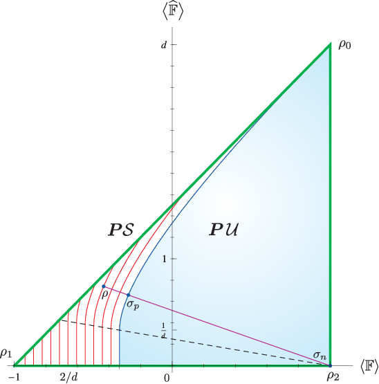
where $({\mathbbm{1}}\pm\mathbb{F})/2$ are the projections onto the symmetric and anti-symmetric subspace, respectively. Consequently, every density operator in $G^{\prime}$ is in the convex hull of the corresponding normalized density matrices $\rho_{i}=P_{i}/\mathrm{tr}[P_{i}]$ of which $\rho_{1}$ corresponds to the Werner-Holevo channel in (15), $\rho_{0}$ is the ideal channel and $\sum_{i}P_{i}/d^{2}$ corresponds to the completely depolarizing channel $T(\rho)=\mathrm{tr}[\rho]\,{\mathbbm{1}}/d$. Clearly, all of them are unital, i.e., elements of $\mathcal{S}$. Every state $\rho\in G^{\prime}$ is completely characterized by its ”coordinates”

$$\left(\left\langle\mathbb{F}\right\rangle,\big\langle\widehat{\mathbb{F}}\big\rangle\right)_{\rho}\equiv\left(\mathrm{tr}\left[\rho\mathbb{F}\right],\mathrm{tr}\left[\rho\widehat{\mathbb{F}}\right]\right).$$

Especially for the extreme points $\rho_{i}$ we obtain (see Fig. 1)

state $\rho_{0}$ $\rho_{1}$ $\rho_{2}$ coords $(1,d)$ $(-1,0)$ $(1,0)$

(16)

We will now determine the subset $\mathcal{U}$ of mixtures of unitary channels within the set of $O(d)$-covariant channels. Following the above considerations this amounts to identifying the corresponding region in the two-dimensional parameter space

$$\begin{split}\mathcal{U}\cap G^{\prime}\cong&\left\{\left(\left\langle\mathbb{F}\right\rangle,\big\langle\widehat{\mathbb{F}}\big\rangle\right)_{\rho}\,:\,\rho\in\mathcal{U}\right\}\\ =\mathrm{conv}&\left\{\left(\left\langle\mathbb{F}\right\rangle,\big\langle\widehat{\mathbb{F}}\big\rangle\right)_{U}\,:\,U\text{ unitary}\right\},\end{split}$$

(17)

where the index $U$ stands for the expectation value w.r.t. $({\mathbbm{1}}\otimes U)\left|\Omega\right\rangle$ which parameterizes an extreme point within $\mathcal{U}$. A short calculation reveals that

$$\begin{split}\left\langle\mathbb{F}\right\rangle_{U}&\equiv\mathrm{tr}\left[\left({\mathbbm{1}}\otimes U\right)\left|\Omega\right\rangle\left\langle\Omega\right|\left({\mathbbm{1}}\otimes U^{\dagger}\right)\mathbb{F}\right]=\frac{1}{d}\,\mathrm{tr}\left[U\overline{U}\right],\\ \big\langle\widehat{\mathbb{F}}\big\rangle_{U}&\equiv\mathrm{tr}\left[\left({\mathbbm{1}}\otimes U\right)\left|\Omega\right\rangle\left\langle\Omega\right|\left({\mathbbm{1}}\otimes U^{\dagger}\right)\widehat{\mathbb{F}}\right]=\frac{1}{d}\,\left\lvert\mathrm{tr}\,U\right\rvert^{2}.\\ \end{split}$$

(18)

The picture depends crucially on whether $d$ is even or odd.

So the interesting structure only emerges for $d$ odd (see Fig. 1 for $d=3$), for which we need the following result proven in appendix VII.2:

The fact that according to Prop. 10, we can restrict to decompositions within the two-dimensional parameter space, together with the explicit characterization of the set $\mathcal{U}\cap G^{\prime}$ enables us now to compute the negativity $\mathcal{N_{U}}$, as follows.

We show first that in Eq. (12), $\sigma_{n}=\rho_{2}$ always obtains the infimum, as illustrated in Fig. 2. Since $\mathcal{U}\cap G^{\prime}$ is convex and closed, the optimal $\sigma_{p,n}$ in (12) are on the boundary of $\mathcal{U}\cap G^{\prime}$, and $\sigma_{n}$ lies either on the segment joining $\rho_{2}$ and $\rho_{0}$ or the one joining $\rho_{2}$ and the covariant state with coordinates $\left(-1+2/d,0\right)$. We may w.l.o.g. assume the former, i.e., $\sigma_{n}=\lambda\,\rho_{0}+(1-\lambda)\rho_{2}$ for a $\lambda\in[0,1]$. Considering decompositions $\rho=\alpha_{p}\,\sigma_{p}-\alpha_{n}\,\sigma_{n}$ with optimal $\sigma_{p}$ (depending on $\lambda$) given $\rho$ and $\sigma_{n}$ via $\lambda$, both $\alpha_{p,n}$ are already determined by the $x$-coordinates of $\rho$ and $\sigma_{p,n}$ due to $\alpha_{p}+\alpha_{n}=1$. Note that the $x$-coordinates of $\rho$ and $\sigma_{n}$ remain fixed for all values of $\lambda$ whereas the $x$-coordinate of $\sigma_{p}$ is non-increasing as $\lambda$ decreases, and so is $\alpha_{n}$. That is, $\lambda=0$ or equivalently $\sigma_{n}=\rho_{2}$ minimizes $\alpha_{n}$.

It follows that a uniform scaling of the boundary of $\mathcal{U}\cap G^{\prime}$ by a factor $\left(1+\alpha_{n}\right)$ starting from $\rho_{2}$ as origin yields precisely the set of points with negativity $\alpha_{n}$.

We may write each $\rho\in\mathcal{S}\setminus\mathcal{U}\cap G^{\prime}$ in terms of a convex combination of the $\rho_{i}$ listed in table 16, that is, $\rho=\sum_{i}q_{i}\,\rho_{i}$ with $q_{i}\geq 0$ and $\sum_{i}q_{i}=1$. From Fig. 2 it is evident that $q_{1}>0$ for all $\rho\notin\mathcal{U}$. Set $q:=q_{0}/q_{1}$ and distinguish the following two cases due to the particular shape of $\mathcal{U}\cap G^{\prime}$.

• •

  $q>\frac{1}{d(d-1)}$. This corresponds exactly to the area above the dashed line in Fig. 2. Applying the scaling $\left(1+\alpha_{n}\right)$ to the curve in theorem 13, an explicit calculation shows that

  	$\displaystyle\mathcal{N_{U}}(\rho)$	$\displaystyle=\frac{1}{d-2}\left(d-1+\left(d+\frac{2}{d-2}\right)q-2\,\frac{d-1}{d-2}\sqrt{q^{2}+\frac{d-2}{d-1}\,q}\right)q_{1}-1,$
  	$\displaystyle\rho$	$\displaystyle=\sum_{i=1}^{3}q_{i}\,\rho_{i}\in\mathcal{S}\setminus\mathcal{U}\ \text{ with }q_{i}\geq 0,\ \sum_{i}q_{i}=1,\quad q:=q_{0}/q_{1}.$

• •

  $q\leq\frac{1}{d(d-1)}$. In this case the negativity does not depend on $q$, and we get

  $$\mathcal{N_{U}}(\rho)=\frac{d}{d-1}\,q_{1}-1.$$

In particular, $\mathcal{N_{U}}(\rho)$ is maximal exactly for the Werner-Holevo channel $\rho_{-}$, namely $\mathcal{N_{U}}\left(\rho_{-}\right)=1/(d-1)$.

As usual we switch to the Jamiolkowski representation, where the family of channels in Eq. (21) becomes

$$\rho_{T}=\left(1-\frac{1}{d}+\frac{\epsilon}{2}\right)\rho_{-}+\left(\frac{1}{d}-\frac{\epsilon}{2}\right)\rho_{\text{+}},\quad d\mbox{ odd}$$

where $\rho_{\pm}$ are the normalized projections onto the symmetric and anti-symmetric subspace, respectively. The parametrization is chosen such that $\rho_{T}\in\mathcal{S}\setminus\mathcal{U}$ for $\epsilon\in(0,2/d]$ since

$$\mathrm{tr}\left[\rho_{T}\mathbb{F}\right]=-1+\frac{2}{d}-\epsilon,$$

and $\mathbb{F}+\left(1-2/d\right){\mathbbm{1}}$ is a tight separation witness according to Thms.7,13. To exploit the full symmetry coming from $\tilde{T}=T$ we follow section V.B of [23] and increment the tensor product symmetry group⁶⁶ 6 The aim is to use the full symmetry group. That is, we use $V\otimes V$, $V\in U(d)$ for $\rho_{T}$ which already allows us to discard $\hat{\mathbb{F}}$ from the commutant. We use further that the commutant of a tensor product is the tensor product of the commutants and that Prop. 10 remains true when adding the additional flip operator. $\left\{(U\otimes U\right)\otimes\left(V\otimes V)\right\}$ by a flip operator which interchanges the tensor factors in the product $T\otimes\tilde{T}$. This results in a larger symmetry group $G$, thus yielding a smaller commutant $G^{\prime}\subset\mathcal{M}_{d^{4}}$ which is spanned by ${\mathbbm{1}}$ and

$$F:=\frac{1}{2}\left({\mathbbm{1}}\otimes\mathbb{F}+\mathbb{F}\otimes{\mathbbm{1}}\right),\quad F_{12}:=\mathbb{F}\otimes\mathbb{F}.$$

That is, every state $\rho\in G^{\prime}$ is now completely characterized by the expectation values/coordinates

$$\left(\left\langle F\right\rangle,\left\langle F_{12}\right\rangle\right)_{\rho}\equiv\left(\mathrm{tr}\left[\rho\,F\right],\mathrm{tr}\left[\rho\,F_{12}\right]\right).$$

Especially for any unitary channel described by $U\in\mathcal{M}_{d^{2}}$, setting $U_{\mathfrak{s}}:=\frac{1}{2}\left(U+U^{T}\right)$ and denoting partial transposes by ${}^{T_{i}}$ gives

$$\begin{split}\left\langle F_{12}\right\rangle_{U}&=\mathrm{tr}\left[F_{12}\left({\mathbbm{1}}\otimes U\right)\left|\Omega\right\rangle\left\langle\Omega\right|\left({\mathbbm{1}}\otimes U^{\dagger}\right)\right]=\frac{1}{d^{2}}\,\mathrm{tr}\left[U\,\overline{U}\right],\\ \left\langle F\right\rangle_{U}&=\mathrm{tr}\left[F\left({\mathbbm{1}}\otimes U\right)\left|\Omega\right\rangle\left\langle\Omega\right|\left({\mathbbm{1}}\otimes U^{\dagger}\right)\right]\\ &=\frac{1}{2\,d^{2}}\,\mathrm{tr}\left[U\left(\overline{U}^{T_{1}}+\overline{U}^{T_{2}}\right)\right]\\ &=\frac{1}{d^{2}}\,\mathrm{tr}\left[U\,\overline{U_{\mathfrak{s}}}^{T_{2}}\right]=\frac{1}{d^{2}}\,\mathrm{tr}\left[U_{\mathfrak{s}}\,\overline{U_{\mathfrak{s}}}^{T_{2}}\right].\\ \end{split}$$

(22)

The last equation uses the fact that $\overline{U_{\mathfrak{s}}}^{T_{2}}$ is again symmetric. The ranges of the expectation values in Eq. (22) are studied in appendix VII.3. In particular for $d=3$ we provide an explicit construction for the coordinates

$$\left(\left\langle F\right\rangle,\left\langle F_{12}\right\rangle\right)_{\vartheta}=\frac{1}{9}\left(-\frac{8}{3}\left(\cos\vartheta+1\right)^{2}+3,\,16\cos^{2}\vartheta-7\right),\quad\vartheta\in\left[0,\pi/2\right]$$

(23)

corresponding to convex combinations of unitary channels. Now matching the coordinates of $T\otimes T$,

$$\left(\left\langle F\right\rangle,\left\langle F_{12}\right\rangle\right)_{T}=\left(\mathrm{tr}\left[\rho_{T}\mathbb{F}\right],\mathrm{tr}\left[\rho_{T}\mathbb{F}\right]^{2}\right)=\left(x,x^{2}\right),\quad x:=-1+\frac{2}{d}-\epsilon$$

with (23) yields

$$\epsilon=\frac{2}{3}\left(4-3\,\sqrt{2}-\sqrt{3}+\sqrt{6}\right)\approx\frac{1}{\sqrt{10}}$$

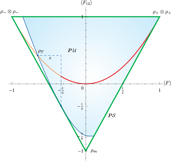
as shown in Fig. 3. The blue area corresponds to convex combinations of unitary channels⁷⁷ 7 A proof that (23) really solves the minimization problem (32) as acclaimed is still outstanding, but strongly supported by numerical tests. In any case, the set of convex combinations of unitary channels is at least as big as the blue area., i.e., elements of $\mathcal{U}$, the orange curve to coordinates of single-channel tensor products and the red part of this curve to the elements of $\mathcal{U}$ on the single-channel level. The state at the lower corner is

$$\rho_{m}=\frac{1}{2}\left(\rho_{-}\otimes\rho_{+}+\rho_{+}\otimes\rho_{-}\right).$$

As can be seen from direct inspection, each point on the curve (23) is an extreme point of the blue area. The remaining extreme points $(1,1)$ and $\left(\frac{1}{9},-\frac{7}{9}\right)$ are realized by the unitaries ${\mathbbm{1}}$ and $\left(\begin{smallmatrix}&-1\\ 1&\end{smallmatrix}\right)^{\otimes 4}\oplus 1$, respectively.

References

• [1] D. Pérez-García, M. M. Wolf, D. Petz, and M.B. Ruskai. Contractivity of positive and trace-preserving maps under LpL_{p} norms. J. Math. Phys., 47(8):083506, 2006.
• [2] A. Arias, A. Gheondea, and S. Gudder. Fixed points of quantum operations. J. Math. Phys., 43(12):5872–5881, 2002.
• [3] C. King. Additivity for unital qubit channels. J. Math. Phys., 43:4641–4653, October 2002.
• [4] M. Fukuda. Simplification of additivity conjecture in quantum information theory. Quant. Inf. Comp., 6:179–186, 2007.
• [5] M. Fukuda and M. M. Wolf. Simplifying additivity problems using direct sum constructions. J. Math. Phys., 48:2101, July 2007.
• [6] B. Rosgen. Additivity and distinguishability of random unitary channels. arXiv:0804.1936, 2008.
• [7] S.L. Tregub. Bistochastic operators on finite-dimensional von-Neumann algebras. Soviet Math., 30:105, 1986.
• [8] B. Kümmerer and H. Maassen. The essentially commutative dilations of dynamical semigroups on MnM_{n}. Commun. Math. Phys., 109:1–22, 1987.
• [9] L. J. Landau and R. F. Streater. On Birkhoff’s theorem for doubly stochastic completely positive maps of matrix algebras. Lin. Alg. Appl., 193:107–127, 1993.
• [10] G. Birkhoff. Three observations on linear algebra. Univ. Nac. Tucuan. Revista A, 5:147–151, 1946.
• [11] M. Gregoratti and R. F. Werner. Quantum lost and found. J. Mod. Opt., 50:915–933, 2003.
• [12] J.A. Smolin, F. Verstraete, and A. Winter. Entanglement of assistance and multipartite state distillation. Phys. Rev. A, 72:052317, 2005.
• [13] A. Jamiolkowski. Linear transformations which preserve trace and positive semidefiniteness of operators. Rep. Math. Phys., 3:275–278, 1972.
• [14] O. Rudolph. On extremal quantum states of composite systems with fixed marginals. J. Math. Phys., 45(11):4035–4041, 2004.
• [15] K.R. Parthasarath. Extremal quantum states in coupled systems. Annales de l’Institut Henri Poincare (B) Probability and Statistics, 41:257–268, 2005.
• [16] Koenraad M. R. Audenaert and Stefan Scheel. On random unitary channels. New J. Phys., 10:023011, 2008.
• [17] Man-Duen Choi. Completely positive linear maps on complex matrices. Lin. Alg. Appl., 10:285–290, 1975.
• [18] F. Buscemi. On the minimal number of unitaries needed to describe a random-unitary channel. Phys. Lett. A, 360:256–258, 2006.
• [19] Eberhard Zeidler. Applied Functional Analysis. Main Principles and Their Applications. Springer New York, 1995.
• [20] D. P. DiVincenzo, C. A. Fuchs, H. Mabuchi, J. A. Smolin, A. V. Thapliyal, and A. Uhlmann. Entanglement of assistance. In Proc. Quantum Computing and Quantum Communications, pages 247–257. First NASA Intl. Conf., Palm Springs, Springer, 1999.
• [21] G. Vidal and R.F. Werner. Computable measure of entanglement. Phys. Rev. A, 65:032314, 2002.
• [22] R.F. Werner and A.S. holevo. Counterexample to an additivity conjecture for output purity of quantum channels. J. Math. Phys., 43:4353–4357, 2002.
• [23] K.G. H. Vollbrecht and R. F. Werner. Entanglement measures under symmetry. Phys. Rev. A, 64:062307, 2001.
• [24] H. Faßbender and Kh. D. Ikramov. Some observations on the Youla form and conjugate-normal matrices. Lin. Alg. Appl., 422:29–38, 2006.
• [25] Open problems in QIT. http://www.imaph.tu-bs.de/qi/problems/.
• [26] Roger A. Horn and Charles R. Johnson. Matrix Analysis. Cambridge University Press, 1990.
• [27] Angelika Bunse-Gerstner, Ralph Byers, and Volker Mehrmann. A quaternion qr algorithm. Numer. Math., 55:83–95, 1989.