Crossover from Attractive to Repulsive Casimir Forces and Vice Versa

Macroscopic bodies that are immersed in a medium frequently experience long-range effective forces originating from fluctuations in the medium. Such fluctuation-induced forces are ubiquitous in nature. A well-known example is the Casimir force between two metallic conducting plates caused by fluctuations of the electromagnetic field [1]. Other important examples are the Casimir forces caused by confined thermal fluctuations, either at critical points [2, 3] or due to Goldstone modes [4]. Although predicted decades ago in a seminal paper by Fisher and de Gennes [2], such so-called “thermodynamic Casimir forces” were verified experimentally in a clear manner only recently — at first, indirectly by the thinning of ⁴He wetting layers near the lambda transition [5] and subsequently by their direct observation in binary fluid mixtures [6]. Current Monte Carlo simulations [7, 8, 6] were able to produce data in conformity with these experiments.

Understanding fluctuation-induced forces is of great interest, for both technical and fundamental reasons. It has recently been realized that quantum electromagnetic Casimir forces must be taken into account when designing micromechanical devices [9]. Analogous as well as thermodynamic Casimir forces are likely to be important also for microfluidic systems [10, 6]. From a general vantage point, one of the most interesting aspects of fluctuation induced forces is their universality: They usually depend only on gross features of the medium, the macroscopic bodies, and the geometry but are independent of microscopic details.

A much studied case is the Casimir force $\mathcal{F}_{C}$ between two macroscopic parallel plates at a distance $L$, acting as boundaries of the medium in the $z$ direction normal to the plates. It is frequently stated that, for a given medium and bulk dimension $d$, this force — and hence its sign — depends on the boundary conditions $\wp$ on both boundary planes. Both the QED Casimir force and the thermodynamic Casimir force at a $d$-dimensional bulk critical point decay as inverse powers of $L$, the former (in three dimension) as $L^{-4}$, the latter as $L^{-d}$. Their strengths are commonly characterized by dimensionless Casimir amplitudes $\Delta^{(\wp)}_{C}$, which are believed to be universal, though boundary condition-dependent [3, 11, 12, 13]. For example, the critical Casimir force (measured in temperature units $k_{B}T$ and per cross-sectional area $A$) is conventionally written as

If the boundary conditions are symmetric so that reflection positivity holds, $\mathcal{F}_{C}$ is guaranteed to be attractive [14] (corresponding to $\Delta^{(\wp)}_{C}<0$); for nonsymmetric boundary conditions, repulsive Casimir forces may occur even for this simple slab geometry.

The aim of this Letter is to show that the above picture is oversimplified. Boundary conditions are scale-dependent properties. This entails that, even on length scales that are large compared to microscopic distances, the strengths of the critical Casimir forces cannot, in general, be characterized by constant universal amplitudes $\Delta^{(\wp)}_{C}$. Rather, the $\Delta^{(\wp)}_{C}$ get replaced by effective scale- (i.e., $L$-) dependent amplitudes. As $L$ increases, they can change considerably. Particularly interesting is that even their signs may change so that originally attractive Casimir forces may turn repulsive as $L$ increases and vice versa. Focusing on the case of critical Casimir forces, we shall present results for the associated scale-dependent amplitudes which show that — under appropriate conditions — smooth crossovers from repulsive to attractive as well as from attractive to repulsive Casimir forces are possible. Such crossovers should be accessible to experimental tests.

To become more specific, let us consider an $n$-component $\phi^{4}$ theory on a slab $\mathfrak{V}=\mathbb{R}^{d-1}\times[0,L]$ bounded in the $z$ direction by a pair of planes $\mathfrak{B}_{1}$ at $z=0$ and $\mathfrak{B}_{2}$ and $z=L$. For simplicity, we assume that these planes do not give rise to interactions breaking the $O(n)$ symmetry of the Hamiltonian $\mathcal{H}$. An appropriate choice then is [15, 11, 12, 13]

where $\int_{\mathfrak{V}}$ and $\int_{\mathfrak{B}_{j}}$ are volume and surface integrals, respectively. This Hamiltonian is well known from the study of surface critical behavior. Let us recall some well-known facts needed below [15].

In Landau theory the Robin boundary conditions

result, where $\partial_{n}$ means a derivative along the inner normal. For $\mathring{c}_{j}=\infty$ they reduce to Dirichlet and for $\mathring{c}_{j}=0$ to Neumann boundary conditions. The physical significance of the interaction constants $\mathring{c}_{j}$ is to account for local changes of the pair interactions near the planes $\mathfrak{B}_{j}$. The larger the $\mathring{c}_{j}$, the stronger is the order parameter $\bm{\phi}$ suppressed at $\mathfrak{B}_{j}$. In Landau theory, $\mathring{c}_{j}=0$ corresponds to the special value $\mathring{c}_{j}=\mathring{c}_{\text{sp}}$ at which the plane $\mathfrak{B}_{j}$ becomes critical exactly at the bulk transition temperature $T_{c,b}$. More precisely, when $\mathring{c}_{j}<\mathring{c}_{\text{sp}}$, a continuous phase transition from a disordered phase to a (bulk-disordered) phase with long-range surface order at $\mathfrak{B}_{j}$ occurs in the semi-infinite ($L=\infty$) system at a temperature $T_{c,s}(\mathring{c}_{j})>T_{c,b}$. The special value $\mathring{c}_{\text{sp}}$ of $\mathring{c}_{j}$ at which $T_{c,s}(\mathring{c}_{\text{sp}})=T_{c,b}$ specifies a surface multicritical point, called “special” on the bulk critical line $\mathring{\tau}=\mathring{\tau}_{c,b}$. In Landau theory, both $\mathring{\tau}_{c,b}$ and $\mathring{c}_{\text{sp}}$ vanish.

Beyond Landau theory, several important changes occur. First, the boundary conditions (3) fluctuate — they hold in an operator sense, i.e., inside of averages [15]. Second, provided the multicritical point exists, — i.e., when $d$ is sufficiently large that long-range surface order is possible at $T>T_{c,b}$ — it gets shifted to nonzero values of $\mathring{\tau}_{c,b}$ and $\mathring{c}_{\text{sp}}$, which depend on microscopical details (lattice constant $a$ etc.).

Thus, for critical enhancement $\mathring{c}_{j}=\mathring{c}_{\text{sp}}$, a Robin boundary condition (3) with a nonuniversal $\mathring{c}_{\text{sp}}$ rather than a Neumann boundary condition applies (on the mesoscopic scale on which a continuum description is appropriate). This does not automatically rule out the validity of a Neumann boundary condition in the large-scale limit $z\to\infty$ with $a\ll z\lesssim\xi$ (where $\xi$ is the bulk correlation length). The behavior of the order parameter near $\mathfrak{B}_{j}$ follows from the boundary operator expansion $\bm{\phi}(\bm{x})\approx C(\Delta z)\,\bm{\phi}\rvert_{\mathfrak{B}_{j}}$, where $\bm{\phi}\rvert_{\mathfrak{B}_{j}}$ is located on $\mathfrak{B}_{j}$ at a distance $\Delta z$ from $\bm{x}$. The short-distance behavior $C(\Delta z)\sim\lvert\Delta z\rvert^{(\beta_{1}^{\text{sp}}-\beta)/\nu}$ is governed by the difference of the scaling dimensions $\beta/\nu$ and $\beta_{1}^{\text{sp}}/\nu$ of $\bm{\phi}$ and $\bm{\phi}\rvert_{\mathfrak{B}_{j}}$, respectively. Only when their difference vanishes does a Neumann boundary condition hold on large length scales. While this is the case when $d$ exceeds the upper critical dimension $d^{*}=4$ (since $\beta=\beta_{1}^{\text{sp}}=1/2$ in Landau theory), it fails when $d<d^{*}$ because $\beta>\beta_{1}^{\text{sp}}$. Thus, neither on mesoscopic nor on large scales does a Neumann boundary condition hold at the special transition when $d<d^{*}$.

Conversely, one may choose $\mathring{c}_{j}=0$, so that a Neumann boundary condition holds on a mesoscopic scale, and inquire again into the large-scale boundary conditions. Now $\mathring{c}_{j}=0$ translates into nonzero deviations $\delta\mathring{c}_{j}\equiv\mathring{c}_{j}-\mathring{c}_{\text{sp}}$ from the multicritical point. Hence the scaling fields $c_{j}\sim\delta\mathring{c}_{j}$ must vary under changes $\mu\to\mu\ell$ of the momentum scale. They become scale-dependent quantities $\bar{c}_{j}(\ell)$ that behave $\sim\ell^{-\Phi/\nu}\,c_{j}$ near $c_{j}=0$, where $\Phi$ and $\nu$ are the familiar surface crossover and bulk correlation length exponents, respectively. Depending on whether $c_{j}>0$ or $c_{j}<0$, they approach the fixed-point values $c^{*}_{\text{ord}}=\infty$ and $c^{*}_{\text{ex}}=-\infty$ at which the fixed points describing the ordinary and extraordinary transitions of semi-infinite systems are located. The short-distance behaviors of $\bm{\phi}$ near $\mathfrak{B}_{j}$ are known in both cases. At the ordinary fixed point $(c_{j}=+\infty$), one has $\bm{\phi}\sim z^{(\beta_{1}^{\text{ord}}-\beta)/\nu}\partial_{n}\bm{\phi}\rvert_{\mathfrak{B}_{j}}$, where $\beta_{1}^{\text{ord}}>\beta$ (for $d<4$ and in Landau, theory where $\beta_{1}^{\text{ord}}=1$); at the extraordinary fixed point ($c_{j}=-\infty$), one has $\bm{\phi}\sim\lvert\Delta z\rvert^{-\beta/\nu}$. Hence, whenever the initial $c_{j}>0$, Dirichlet boundary conditions hold asymptotically on large length scales at $\mathfrak{B}_{j}$. The upshot is that, for generic values of $\mathring{c}_{j}\in(-\infty,\infty)$ and mesoscale boundary conditions (3), the boundary conditions of the full interacting theory will change under scale transformations, even in the Neumann case $\mathring{c}_{j}=0$.

To elucidate the consequences for the critical Casimir force, recall that the reduced free energy of the slab per cross-sectional area $A\to\infty$ can be decomposed as

into contributions from the bulk density $f_{b}$, the surface excess density $f_{s}$, and an $L$-dependent residual part $f_{\text{res}}(L)$. The behavior of these quantities at $T_{c,b}$ can be analyzed via field-theoretic renormalization group (RG) methods. The RG equations satisfied by $f_{b}$ and $f_{s}$ upon renormalization at $d<d^{*}$ are inhomogeneous. However, the one of $f_{\text{res}}(L)$ is known to be homogeneous [15, 11, 12, 13]. Solving it at $T_{c,b}$ yields the scaling form

where the $c_{j}$ now denote renormalized quantities $c_{j}=\mu^{-1}Z_{c}^{-1}\delta\mathring{c}_{j}$ involving a familiar renormalization factor $Z_{c}$ of Ref. [15]. The function $D(\mathsf{c}_{1},\mathsf{c}_{2})$ is universal (up to nonuniversal metric factors). It replaces the amplitude $\Delta^{(\wp)}_{C}/n$ in the first form of Eq. (1), while the critical Casimir force becomes

with

We have computed the functions $D$ and $\mathcal{D}$ in $d=4-\epsilon$ dimensions for general nonnegative values of $\mathsf{c}_{1}$ and $\mathsf{c}_{2}$ to two-loop order, using $\epsilon$ as a small parameter. The required free-energy terms involve summations over the spectrum $\{k_{m}^{2}\}$ of the operator $-\partial_{z}^{2}$ on $[0,L]$. The discrete values $k_{m}$ are fixed by the boundary conditions (3) and depend on $\mathring{c}_{1}$, $\mathring{c}_{2}$, and $L$. We evaluated such mode sums by means of complex integration, employing a variant of Abel-Plana techniques that facilitated the separation of bulk and surface terms [16].

To present our results, we introduce the functions

and the polynomials

Then our result for $D$ can be written as

where $\gamma$ is the Euler-Mascheroni constant.

To check this result, one can set $(c_{1},c_{2})$ to $(\infty,\infty)$, $(\infty,0)$, and $(0,0)$ and confirm by analytic calculation of the required integrals that the respective series (12) reduce to the $O(\epsilon)$ results of Ref. [11] for the amplitudes $\Delta^{(\text{ord,ord})}_{C}/n$, $\Delta^{(\text{ord,sp})}_{C}/n$, and $\Delta^{(\text{sp,sp})}_{C}/n$. Note that the case $(c_{1},c_{2})=(0,0)$ is special: Unlike $\Delta^{(\text{ord,ord})}_{C}$ and $\Delta^{(\text{ord,sp})}_{C}$, the amplitude $D(0,0)$ does not have an expansion in integer powers of $\epsilon$ but involves also half-integer powers $\epsilon^{k/2}$, with $k\geq 3$ (besides powers of $\ln\epsilon$ when $k>3$) [12].

In Fig. 1, we show a plot of $D(\mathsf{c}_{1},\mathsf{c}_{2})$ for the $d=3$ Ising case $n=1$. It was obtained by numerical evaluation of the $O(\epsilon)$ result (12) at $\epsilon=n=1$.

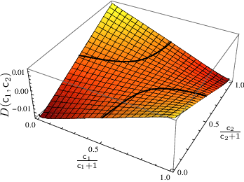
As one sees, $D$ changes sign along certain paths. The same is true for the scaling function (7), and hence for the critical Casimir force $\mathcal{F}_{C}$. Moreover, such sign changes of $\mathcal{F}_{C}$ occur upon increasing $L$ provided $(c_{1},c_{2})$ have appropriate values. That crossovers from attractive to repulsive Casimir forces and vice versa can occur is illustrated in Fig. 2.

To put these results in perspective, consider the case $\mathring{c}_{1}=0$. Here a Neumann boundary condition holds at $\mathfrak{B}_{1}$ for the regularized theory on the mesoscopic scale on which the continuum description applies. One can derive this model from a simple cubic lattice spin model whose ferromagnetic nearest-neighbor bonds $J_{\bm{x}\bm{x}^{\prime}}$ have strengths $J_{j}$ ($j=1,2$) and $J$, depending on whether both sites $\bm{x}$ and $\bm{x}^{\prime}$ belong to $\mathfrak{B}_{j}$ or at least one of them is not a boundary site. From the known (approximate) relation between $\mathring{c}_{j}$ and $J_{j}/J$ [15], one sees that at $d=3$ the value $(J_{1}/J)_{0}=5/4$ corresponds to $\mathring{c}_{j}=0$. This is less than the value $\rho_{\text{sp}}=1.500(4)$ at which the multicritical point of the $d=3$ Ising model is located according to Monte Carlo simulations [17]. Thus, a mesoscopic Neumann boundary condition at $\mathfrak{B}_{j}$ corresponds to a subcritical enhancement $c_{j}>0$. As explained, a Dirichlet boundary condition applies in such a situation on large length scales.

A similar crossover $\mathsf{c}_{2}=c_{1}L^{\Phi/\nu}\to\infty$ occurs also for the choice $c_{2}=0.1$ made in Fig. 2. In regimes where $\mathsf{c}_{1}$ and $\mathsf{c}_{2}$ are both small or both large, $\mathcal{F}_{C}$ must be attractive. Yet in regimes where $\mathsf{c}_{1}$ is sufficiently small while $\mathsf{c}_{2}$ is large, $\mathcal{F}_{C}$ is repulsive. Depending on our choices $c_{1}=0$ and $c_{1}=10$ ($\gg c_{2}$), crossovers from attractive to repulsive Casimir forces and vice versa occur.

These predictions should be testable by Monte Carlo simulations for three-dimensional Ising models of the kind described above and studied in Ref. [17]. Ideal experimental systems to measure the calculated scaling function would satisfy three criteria: (i) order-parameter dimension $n=1$; (ii) non-symmetry-breaking boundaries; (iii) tunability of the effective boundary pair interactions ($\mathring{c}_{1}$ and $\mathring{c}_{2}$). In the case of ⁴He at the lambda transition, the boundaries do not break the $O(2)$ symmetry. However, a two-component order parameter is involved, a long-range ordered surface phase should not be possible at $d=3$, and it is unclear to us how the parameters $\mathring{c}_{j}$ can be varied. Experimental studies of binary liquid mixtures seem to us a more promising alternative. For them, (i) is evidently satisfied. Since walls usually favor one or the other component, the $\mathbb{Z}_{2}$ symmetry is broken by linear boundary terms $-\int_{\mathfrak{B}_{j}}h_{j}\phi$, where each $h_{j}$ can have either sign. It was demonstrated in Ref. [18] that the values of these fields $h_{j}$ can be changed by chemically modifying the surface. It is also known that different signs of $h_{j}$ can be realized by proper choices of the mixtures and substrates [19]. Hence it should be possible to realize experimental setups with $h_{1}$ and $h_{2}$ small and of opposite signs, or with $h_{1}\approx 0$ and $h_{2}$ large and of equal signs. In both cases, sign-changing crossovers of the critical Casimir forces may be expected as $L$ grows. The associated scaling functions would need separate calculations.

Partial support by DFG under grant Di 378/5 is gratefully acknowledged.

References

- [1] H. B. G. Casimir, Proc. K. Ned. Akad. Wet. B51, 793 (1948).
- [2] M. E. Fisher and P.-G. de Gennes, C. R. Séances. Acad. Sci. Série B 287, 207 (1978).
- [3] For background and lists of references, see M. Krech, Casimir Effect in Critical Systems (World Scientific, Singapore, 1994); J. G. Brankov, D. M. Dantchev, and N. S. Tonchev, Theory of Critical Phenomena in Finite-Size Systems — Scaling and Quantum Effects (World Scientific, Singapore, 2000).
- [4] M. Kardar and R. Golestanian, Rev. Mod. Phys. 71, 1233 (1999).
- [5] R. Garcia and M. H. W. Chan, Phys. Rev. Lett. 83, 1187 (1999).
- [6] C. Hertlein, A. Gambassi, S. Dietrich, and C. Bechinger, Nature 451, 172 (2008).
- [7] A. Hucht, Phys. Rev. Lett. 99, 185301 (2007).
- [8] O. Vasilyev, A. Gambassi, A. Maciołek, and S. Dietrich, Europhys. Lett. 80, 60009 (2007).
- [9] H. B. Chan, V. A. Aksyuk, R. N. Kleiman, D. J. Bishop, and F. Capasso, Science 291, 1941 (2001); Phys. Rev. Lett. 87, 211801 (2001); for earlier work on micromechanical systems, see F. Serry, D. Walliser, and G. Maclay, J. Microelectromech. Syst. 4, 193 (1995).
- [10] J. N. Munday and F. Capasso, Phys. Rev. A 75, 060102(R) (2007); for further discussion of the agreement of this work’s experimental data and Lifshitz theory, see B. Geyer, G. L. Klimchitskaya, U. Mohideen, and V. M. Mostepanenko, Phys. Rev. A 77, 036102 (2008) and J. N. Munday and F. Capasso, Phys. Rev. A 77, 036103 (2008).
- [11] M. Krech and S. Dietrich, Phys. Rev. Lett. 66, 345 (1991); Phys. Rev. A 46, 1886 (1992).
- [12] H. W. Diehl, D. Grüneberg, and M. A. Shpot, Europhys. Lett. 75, 241 (2006), cond-mat/0605293.
- [13] D. Grüneberg and H. W. Diehl, Phys. Rev. B 77, 115409 (2008), arXiv:0710.4436.
- [14] C. P. Bachas, J. Phys. A: Math. & Gen. 40, 9089(2007); O. Kenneth and I. Klich, Phys. Rev. Lett. 97, 160401 (2006).
- [15] For background on boundary critical phenomena, see H. W. Diehl, in Phase Transitions and Critical Phenomena, edited by C. Domb and J. L. Lebowitz (Academic, London, 1986), vol. 10, pp. 75–267; Int. J. Mod. Phys. B 11, 3503 (1997), cond-mat/9610143.
- [16] Details will be published elsewhere.
- [17] D. P. Landau and K. Binder, Phys. Rev. B 41, 4633 (1990); C. Ruge, S. Dunkelmann, and F. Wagner, Phys. Rev. Lett. 69, 2465 (1992); M. Pleimling and W. Selke, Eur. Phys. J. B 1, 385 (1998).
- [18] N. S. Desai, S. Peach, and C. Franck, Phys. Rev. E 52, 4129 (1995).
- [19] M. Fukuto, Y. F. Yano, and P. S. Pershan, Phys. Rev. Lett. 94, 135702 (2005); S. Rafai, D. Bonn, and J. Meunier, Physica A 386, 31 (2007).