No. 176, 2008
Electronic Structure of Multilayer Graphene
Abstract
We study the electronic structure of multilayer graphene using a -orbital continuum model with nearest-neighbor intralayer and interlayer tunneling. Using degenerate state perturbation theory, we show that the low-energy electronic structure of arbitrarily stacked graphene multilayers consists of chiral pseudospin doublets with a conserved chirality sum.
1 Introduction
The recent explosion[1, 2] of research on the electronic properties of single layer and stacked multilayer graphene sheets has been driven by advances in material preparation methods[3, 4], by the unusual[5, 6, 7] electronic properties of these materials including unusual quantum Hall effects[8, 9], and by hopes that these elegantly tunable systems might be useful electronic materials.
In this paper[10], we study the electronic structure of arbitrarily stacked multilayer graphene using a -orbital continuum model with only near-neighbor interactions, analyzing its low-energy spectrum using degenerate state perturbation theory. Here we focus solely on aligned multilayer graphene without rotational stacking faults[11]. Interestingly, we find that the low-energy effective theory of multilayer graphene is always described by a set of chiral pseudospin doublets with a conserved chirality sum. We discuss implications of this finding for the quantum Hall effect in multilayer graphene.
2 -orbital continuum model
We consider the -orbital continuum model for -layer graphene Hamiltonian which describes bands near the hexagonal corners of the triangular lattice Brillouin zone, the and points:
| (1) |
where and is an electron annihilation operator for layer , sublattice and momentum measured from or point.
The simplest model for a multilayer graphene system allows only nearest-neighbor intralayer hopping and the nearest-neighbor interlayer hopping . The in-plane Fermi velocity is related with by , where is a lattice constant of monolayer graphene. Although this model is not fully realistic, some aspects of the electronic structure can be understood by fully analyzing the properties of this simplified model first and then considering corrections.
2.1 Stacking diagrams
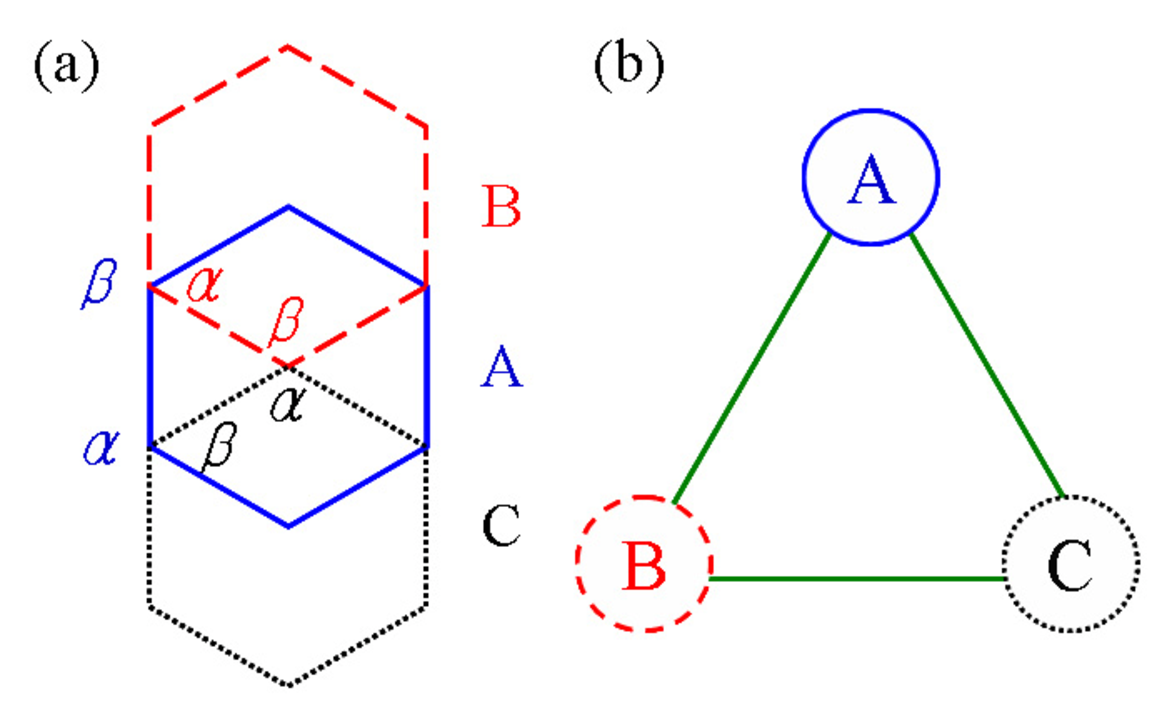
When one graphene layer is placed on another, it is energetically favorable[12] for the atoms of either or sublattices to be displaced along the honeycomb edges, as illustrated in Fig. 1. This stacking rule implies the three distinct but equivalent projections (labeled A, B, and C) of the three-dimensional structure’s honeycomb-lattice layers onto the - plane and distinct -layer stack sequences. When a B layer is placed on an A layer, a C layer on a B layer, or an A layer on a C layer, the sites of the upper layer are above the sites of the lower layer and therefore linked by the nearest interlayer neighbor -orbital hopping amplitude . For the corresponding anticyclic stacking choices (A on B, B on C, or C on A), it is the sites of the upper layer and the sites of the lower layer that are linked. All distinct , , and layer stacks are illustrated in Fig. 2, in which we have arbitrarily labeled the first two layers starting from the bottom as A and B.

2.2 Energy band structure
2.2.1 Preliminaries
Before analyzing energy spectrum of multilayer graphene, let us consider the Hamiltonian of a one-band tight-binding model for a chain of length with near-neighbor hopping parameter :
| (2) |
This Hamiltonian is important for analyzing the role of interlayer hopping as we explain below.
Let be an eigenvector with an eigenvalue . Then the eigenvalue problem reduces to the following difference equation
| (3) |
with the boundary condition . Assuming , it can be shown that[13]
| (4) |
where is the chain eigenvalue index and . Note that odd chains have a zero-energy eigenstate with an eigenvector that has nonzero amplitudes, constant in magnitude and alternating in sign, on the sublattice of the chain ends.
2.2.2 AA stacking
Although AA stacking is not energetically favorable, it is still interesting to consider this arrangement for pedagogical purposes. In the case of AA stacking, the Hamiltonian at is given by
| (5) |
where .
As we now explain, the electronic structure of AA stacked -layer graphene can be thought of as consisting of separate 1D chains for each wavevector in the 2D triangular lattice Brillouin zone of a single graphene layer. For an eigenvector with an eigenvalue and fixed 2D momentum, the difference equations in this case are
| (6) |
with the boundary condition .
Let and where , then
| (7) |
with the same boundary condition . Thus the energy spectrum is given by
| (8) |
where . Note that for odd , the mode provides two zero-energy states at .


Figure 3 shows the band structure of AA stacked trilayer and tetralayer graphene near the point. Because of the hybridization between - and - sublattices in each layer, zero-energy states occur at momenta that are remote from the and points. In the following we turn our attention to stacks in which adjacent graphene layers have a relative rotation of 60 degrees. As we show, in this case the zero-energy states always occur precisely at the Brillouin-zone corners.
2.2.3 AB stacking
In the case of AB stacking, the Hamiltonian at has the following form,
| (9) |
We will see that the subtle difference in the Hamiltonian compared to the AA case changes the electronic structure in a qualitative way. To obtain the energy spectrum of AB stacked -layer graphene, let us consider corresponding difference equations[14]:
| (10) |
with the boundary condition .
Let and , then the difference equations reduce to
| (11) |
with the boundary condition . Then the energy spectrum is given by
| (12) |
where . Thus
| (13) |
Note that relativistic energy spectrum for a particle with the momentum and mass is given by
| (14) |
Thus we can identify as the effective mass for mode .
For a massive mode with mass , the low-energy spectrum is given by
| (15) |
For odd , the mode with is massless and its energy is given by
| (16) |
For even , all modes are massive at low energies. Therefore, the low-energy spectrum with odd number of layers is a combination of one massless Dirac mode and massive Dirac modes, whereas the low-energy spectrum with even number of layers is composed of only massive Dirac modes.


Figure 4 shows the band structure of AB stacked trilayer and tetralayer graphene near the point. As discussed earlier, the trilayer has one massless mode and two massive modes, while the tetralayer has all massive modes at low energies. Note that at , each massless mode gives two zero energies while each massive mode gives one zero energy. Therefore, for odd , there are zero-energy states while for even , there are zero-energy states.
2.2.4 ABC stacking
In the case of ABC stacking, the Hamiltonian at is given by
| (17) |
Unfortunately for ABC stacking, there do not exist low-order difference equations with a simple boundary condition. Instead we can easily derive a low-energy effective Hamiltonian. Surprisingly, it turns out that ABC stacked -layer graphene is described by -chiral 2D electron system. (More detailed discussion for the effective theory of arbitrarily stacked graphene will be presented in §3.)
It is important to recognize that in ABC stacking, there is vertical hopping between all the lower layer sites and all the upper layer sites. For each - pair forms a symmetric-antisymmetric doublet with energies , leaving the bottom and top sites as the only low-energy states. This behavior is readily understood from the stacking diagrams, in Fig. 2. It is possible to construct a -dependent low-energy effective Hamiltonian for the low-energy part of the spectrum using perturbation theory. The same procedure can then be extended to arbitrary stacking sequences.
The simplest example is bilayer graphene[15]. Low and high energy subspaces are identified by finding the spectrum at and identifying all the zero-energy eigenstates. The intralayer tunneling term, which is proportional to , couples low and high energy states. Using degenerate state perturbation theory, the effective Hamiltonian in the low energy space is given to leading (2nd) order in by
| (18) |
where we have used a basis, and . In the same way we find that the effective Hamiltonian of ABC stacked -layer graphene is given by
| (19) |
using a basis. The leading correction appears at order in because the unperturbed high-energy states are localized on a pair and the perturbation is intralayer tunneling. Note that we have for mathematical convenience chosen a gauge in which the single-layer Hamiltonian is
| (20) |
We can prove Eq. (19) by the mathematical induction method. Imagine that we add one more layer on top of -layer graphene with ABC stacking. Then the combined Hamiltonian is given by
| (21) |
using a basis.
Let be a low-energy subspace spanned by and be a high-energy subspace spanned by . Note that the effective Hamiltonian can be derived using the degenerate state perturbation theory[16],
| (22) |
Here the projected Hamiltonian matrices to and subspace are given by
| (23) |
and . Thus we can easily show that,
| (24) |
which proves Eq. (19). The corresponding energy spectrum in Eq. (19) is given by
| (25) |


Figure 5 shows the band structure of ABC stacked trilayer and tetralayer graphene near the point. Note that at , there are only two zero energy states no matter how thick the stack is.
2.2.5 Arbitrary stacking
It is easy to generalize the previous discussion to construct the Hamiltonian for an arbitrarily stacked multilayer graphene system.


Figure 6 shows the band structure of ABCB stacked tetralayer graphene and ABBC stacked tetralayer graphene near the point. For the ABCB stacked tetralayer graphene, the low-energy spectrum looks like a superposition of a linear dispersion and a cubic one. For the ABBA stacked tetralayer graphene, zero energies appear not only at the Dirac point but also away from it. A more detailed low-energy spectrum analysis will be presented in §3.
2.3 Landau level spectrum
2.3.1 Preliminaries
In the presence of a magnetic field , a Hamiltonian is modified by , where is the vector potential with . The quantum Hamiltonian is most easily diagonalized by introducing raising and lowering operators, and substitution, where , and noting that . We can then expand the wavefunction amplitude on each sublattice of each layer in terms of parabolic band Landau level states which are eigenstates of the . For many Hamiltonians, including those studied here, the Hamiltonian can be block diagonalized by fixing the parabolic band Landau-level offset between different sublattices and between different layers. This procedure is familiar from theories of Landau-level structure in other multiband theories.
2.3.2 AA stacking
In the case of AA stacking, let us choose the -th Landau level basis at as
.
Then Eq. (5) reduces to
| (26) |
where . Note that 2D Landau level states with a negative index do not exist so the corresponding basis states and matrix elements are understood as being absent in the matrix block. Thus is a matrix, while is a matrix.
By diagonalizing Eq. (26) using the difference equation method, we can obtain the exact Landau level spectrum. For , Landau levels are given by
| (27) |
where . Note that for , Landau levels are given by . Thus for odd , there exists one (-independent) zero-energy Landau level at .


Figure 7 shows the Landau levels of AA stacked trilayer and tetralayer graphene as a function of magnetic fields. For the trilayer, there is one zero-energy Landau level, while for the tetralayer, there is no zero-energy Landau level. Note that there are Landau levels crossing the zero-energy line in AA stacking.
2.3.3 AB stacking
In the case of AB stacking, a proper choice of the -th Landau level basis at is such that all the interlayer hopping terms are contained in the -th Landau level Hamiltonian. Then Eq. (9) reduces to
| (28) |
where . As discussed earlier, special care should be given for states with a negative index.
For the Hamiltonian in Eq. (28), there do not exist corresponding difference equations with a proper boundary condition, thus cannot be diagonalized analytically. From Eq. (15), however, we can find the low-energy Landau levels for massive mode with mass as
| (29) |
where and , which is proportional to . These equations apply at small , just as the limiting low-energy dispersions applied at small momentum . For the massless mode, from Eq. (16) Landau levels are given by
| (30) |
which is proportional to .


Figure 8 shows the Landau levels of AB stacked trilayer and tetralayer graphene as a function of magnetic fields. Note that the linear dependence expected for massive modes applies over a more limited field range when the mass is small. For the trilayer, Landau levels are composed of massless Dirac spectra () and massive Dirac spectra (), while for the tetralayer, Landau levels are all massive Dirac spectra. This is consistent with the band structure analysis shown in Fig. 4.
Note that the massive modes in Eq. (29) have two zero-energy Landau levels for and , whereas the massless mode in Eq. (30) has one for . There are therefore zero-energy Landau levels in both even and odd AB stacks. This property can also be understood directly from the Hamiltonian in Eq. (28), by eliminating negative basis states and rearranging rows to block diagonalize the matrix.
2.3.4 ABC stacking
In the case of ABC stacking, a proper choice of the -th Landau level basis at is
such that all the interlayer hopping terms are contained in the -th Landau level Hamiltonian.
Then Eq. (17) reduces to
| (31) |
where .
The low-energy spectrum can be obtained from the effective Hamiltonian in Eq. (19). For , Landau levels are given by
| (32) |
where , while for they are zero. Note that there are zero-energy Landau levels for ABC stacked -layer graphene.


Figure 9 shows the Landau levels of ABC stacked trilayer and tetralayer graphene as a function of magnetic fields. For the trilayer, Landau levels are proportional to , while for the tetralayer, Landau levels are proportional to .
2.3.5 Arbitrary stacking
It is straightforward to generalize the previous discussion to construct the Hamiltonian in Landau level basis for an arbitrarily stacked multilayer graphene system. As discussed earlier, special care should be given for states with a negative index.


Figure 10 shows Landau levels of ABCB stacked tetralayer graphene and ABBC stacked tetralayer graphene. For the ABCB stacked tetralayer graphene, the Landau levels look like a superposition of and levels, which is consistent with Fig. 6(a). For the ABBA stacked tetralayer graphene, there are Landau levels crossing the zero-energy line, which is consistent with Fig. 6(b). Detailed low-energy Landau-level spectrum analysis will be presented in §3.
2.4 Quantum Hall conductivity
Applying the Kubo formula to a disorder-free systems we find that the conductivity tensor with an external magnetic field along is given by
| (33) |
where is Fermi factor of -th energy state, and
| (34) |
Here is a velocity operator obtained by taking a derivative of the Hamiltonian with respect to . Note that in case of multilayer graphene, the velocity operator is constant, i.e. it does not depend on the Landau level index.
The appropriate quantized Hall conductivity is obtained by evaluating . Detailed analysis of the quantum Hall conductivity will be presented in §3.
3 Chiral decomposition of energy spectrum
In this section11 1 The content of this section provides a more complete explanation of the arguments presented earlier in Ref. 10). we demonstrate an unanticipated low-energy property ofgraphene multilayers, which follows from an interplay between interlayer tunneling and the chiral properties of low-energy quasiparticles in an isolated graphene sheet. Our conclusions apply in the strongest form to models with only nearest-neighbor interlayer tunneling, but are valid over a broad field range as we explain below. We find that the low-energy band structure of any graphene multilayer consists of a set of independent pseudospin doublets. Within each doublet, the bands are described by a pseudospin Hamiltonian of the form
| (35) |
where is a Pauli matrix acting on the doublet pseudospin, is an envelope function momentum measured from either the or corner of the honeycomb lattice’s Brillouin-zone[1, 2], , and is the orientation of . The sign in Eq. (35) assumes the opposite signs in graphene’s and valleys. Following the earlier work on graphene bilayers[15], we refer to as the chirality index of a doublet. In the presence of a perpendicular magnetic field , yields Landau levels at and levels with . Taking the twofold spin and valley degeneracies into account, the number of independent zero-energy band eigenstates at the Dirac point () is therefore , where is the number of pseudospin doublets. We find that, although depends on the details of the stacking sequence,
| (36) |
in an -layer stack. It follows from Eq. (36) that the Hall conductivity of an -layer stack has strong integer quantum Hall effects with plateau conductivities,
| (37) |
where is a non-negative integer.
3.1 Partitioning rules
The low-energy band and the Landau level structure can be read off the stacking diagrams illustrated in Fig. 2 by partitioning a stack using the following rules, which are justified in the following section.
(i) Identify the longest nonoverlapping segments within which there are no reversals of stacking sense. When there is ambiguity in the selection of nonoverlapping segments, choose the partitioning which incorporates the largest number of layers. Each segment (including for interior segments the end layers at which reversals take place) defines a -layer partition of the stack and may be associated with a chirality doublet.
(ii) Iteratively partition the remaining segments of the stack into smaller elements, excluding layers contained within previously identified partitions, until all layers are exhausted.
The chirality decompositions which follow from these rules are summarized in Table 1. Note that this procedure can result in doublets associated with separated single layers which remain at the last step in the partitioning process.
In applying these rules, the simplest case is cyclic ABC stacking for which there are no stacking sense reversals and therefore a single partition. In the opposite limit, AB stacking, the stacking sense is reversed in every layer and the rules imply partitions with for even , and when is odd a remaining partition. Between these two limits, a rich variety of qualitatively distinct low-energy behaviors occur. For example, in the ABCB stacked tetralayer, ABC is identified as a doublet and the remaining B layer gives a doublet. The low-energy band structure and the Landau level structure of this stack, as illustrated in Figs. 6(a) and 10(a), have two sets of low-energy bands with , Landau levels with , and four zero-energy Landau levels per spin and valley. All these properties are predicted by the partitioning rules. We have explicitly checked that the rules correctly reproduce the low-energy electronic structure for all stacking sequences up to . Because each layer is a member of one and only one partition, the partitioning rules imply the chirality sum rule in Eq. (36).
| stacking | chirality | stacking | chirality |
|---|---|---|---|
| ABC | 3 | ABCABC | 6 |
| ABA | 2+1 | ABCABA | 5+1 |
| ABCACA | 4+2 | ||
| ABCA | 4 | ABCACB | 4+2 |
| ABCB | 3+1 | ABCBCA | 3+3 |
| ABAB | 2+2 | ABCBCB | 3+2+1 |
| ABAC | 1+3 | ABCBAB | 3+2+1 |
| ABCBAC | 3+3 | ||
| ABCAB | 5 | ABABCA | 2+4 |
| ABCAC | 4+1 | ABABCB | 2+3+1 |
| ABCBC | 3+2 | ABABAB | 2+2+2 |
| ABCBA | 3+2 | ABABAC | 2+1+3 |
| ABABC | 2+3 | ABACAB | 2+1+3 |
| ABABA | 2+2+1 | ABACAC | 1+3+2 |
| ABACA | 1+3+1 | ABACBC | 1+4+1 |
| ABACB | 1+4 | ABACBA | 1+5 |
3.2 Degenerate state perturbation theory
We start from the well-known massless Dirac equation[1, 2] model for isolated sheets,
| (38) |
where and is the quasiparticle velocity. In the presence of an external magnetic field, and are proportional to the Landau level raising and lowering operators, so that Eq. (38) implies the presence of one macroscopically degenerate Landau level at the Dirac point for each spin and valley, and therefore, to the quantum Hall effect[8, 9] of Eq. (37). An -layer stack has a two-dimensional band structure with atoms per unit cell. The Hamiltonian can be written as
| (39) |
where accounts for interlayer tunneling and for intralayer tunneling. is the direct product of massless Dirac model Hamiltonians for the sublattice pseudospin degrees of freedom of each layer. We construct a low-energy Hamiltonian by first identifying the zero-energy eigenstates of and then treating as a perturbation.
Referring to Fig. 2, we see that is the direct product of a set of finite-length 1D tight-binding chains, as shown in Eq. (4), and a null matrix with dimension equal to the number of isolated sites. The set of zero-energy eigenstates of consists of the states localized on isolated sites and the single zero-energy eigenstates of each odd-length chain.
The low-energy effective Hamiltonian is evaluated by applying leading order degenerate state perturbation theory to the zero-energy subspace. The matrix element of the effective Hamiltonian between degenerate zero-energy states and is given by[16]
| (40) |
where is the smallest positive integer for which the matrix element is nonzero, and , is a projection operator onto the zero-energy subspace. To understand the structure of this Hamiltonian, it is helpful to start with some simple examples.
3.2.1 ABC stacking
For ABC stacked -layer graphene, the zero-energy states are the two isolated site states in bottom and top layers, and . sets of two-site chains form high-energy states. Because is diagonal in layer index and (and hence ) can change the layer index by one unit, the lowest order at which and are coupled is .
3.2.2 AB stacking
For AB stacked -layer graphene, the high-energy Hilbert space consists of a single -site 1D chain, excluding its zero-energy eigenstate when is odd. There is an isolated site in each layer which is connected to both its neighbors at order forming an isolated site chain. When is even, this chain is diagonalized by , doublets formed between -sublattice and -sublattice chain states[14, 17, 18, 19]. When is odd, the zero-energy chain state is mapped to an equal-magnitude oscillating-sign linear combination of isolated site states by intralayer tunneling at order , yielding a doublet. The , doublets are then formed between -sublattice and -sublattice isolated site chain states in the orthogonal portion of the isolated state subspace.
Let us consider the low-energy spectrum of AB stacking in more detail. From Eq. (4) energy spectra and wavefunctions of the single -site chain are given by
| (44) |
where and .
First, let us consider the case with even . Then the low-energy states come from the isolated sites or equivalently their superpositions. Let us define
| (45) |
such that
| (46) |
where . Then the matrix elements between the low-energy states are given by the second order perturbation theory:
| (47) |
Note that and these two modes form a 2-chiral system with energies . The chirality can be manifested clearly if we define
| (48) |
Then the Hamiltonian of the 2-chiral system for is given by
| (49) |
in a basis with . Thus the system is described by a combination of massive Dirac modes with different masses.
For odd , there is a zero-energy state in the -site chain at in Eq. (44). Thus in addition to the massive modes, there exists one massless Dirac mode,
| (50) |
Thus the system is described by one massless Dirac mode and a combination of massive Dirac modes with different masses.
3.2.3 ABC+B type stacking
A more complex and more typical example is realized by placing a single reversed layer on top of ABC stacked -layer graphene with . Note that the last chain has three sites, thus it has a zero-energy state defined by
| (51) |
and two high-energy states with energies defined by
| (52) |
where . Then the first-order perturbation theory gives
| (53) |
suggesting the existence of the massless Dirac mode with a reduced velocity.
Similarly as Eq. (42), we obtain
| (54) |
using a basis. The first block in Eq. (54) gives a doublet with a reduced velocity. Note that the matrix in Eq. (54) is not block diagonal thus we cannot simply say that the second matrix block is a -chiral system. The doublet in this instance includes both the subspace contribution and an equal contribution due to perturbative coupling to the subspace. Using a similar perturbation theory shown in Eq. (22), we can obtain higher order correction by integrating out the massless Dirac mode which forms a higher energy state. Then the final Hamiltonian is reduced to
| (55) |
where
| (56) |
This means that the combined system can be described by a combination of one -chiral system with reduced velocity and one -chiral system. Note that stacking a layer with an opposite handedness partitions a system into systems with different chiralities.
3.2.4 Arbitrary stacking
The relationship between the electronic structure of a general stack and the partitioning procedure explained above can be understood as follows.
(i) First, note that a partition with chirality has isolated sites in its terminal layers that are coupled at order in perturbation theory. In the case of partition, the chain opposite to the single isolated site always has an odd length and provides the zero-energy partner; isolated site to chain coupling therefore always occurs at first order.
(ii) Next, consider the perturbation theory, truncating at successively higher orders. When truncated at first order, the partitions are isolated by higher blocks within which the Hamiltonian vanishes. Each partition therefore yields a separate massless Dirac equation with velocities22 2 The velocity of the doublets is determined by the strength of the coupling between the odd-length chain zero-energy state and isolated states on the sublattice opposite to the chain ends. For a chain of length , the chain’s zero-energy state has nonzero amplitude on the odd-index sites. The velocity is reduced from the single sheet velocity by a factor of , where is the number of isolated sites opposite to the odd-index sites. In a similar manner, higher doublet Hamiltonians are sometimes altered by a multiplicative factor by perturbative coupling to smaller doublets as in the single reversed layer example. that can be smaller than the graphene sheet Dirac velocity. When the perturbation theory is truncated at second order, the Hamiltonian becomes nonzero within the partitions. The eigenenergies within the partitions are parametrically larger, and the Hamiltonian within the partitions is still zero. To leading order therefore, the partitions are separated, and their isolated states are coupled at the second order in perturbation theory so that each provides a doublet such as that of an isolated bilayer. If two or more partitions are adjacent, then their Hamiltonians do not separate. In this case, there is a chain of second order couplings between isolated states, such as those of an even-length AB stack, but the end result is still doublet for each partition.
(iii) The identification between partitions and chiral doublets can be established by continuing this consideration up to the highest values of which occur for a particular stack.
(iv) Then, the effective Hamiltonian of any -layer graphene is as follows:
| (57) |
with the sum rule in Eq. (36). Note that is half the sum of the number of isolated sites and the number of odd-length chains.
3.3 Discussion
3.3.1 Effects of remote hopping
The minimal model we have used to derive these results is approximately valid in the broad intermediate magnetic field range between and T, over which the intralayer hopping energy in field ( where is the magnetic length) is larger than the distant neighbor interlayer hopping amplitudes that we have neglected ( meV), but still smaller than . For example, if we consider hopping process in ABA stacked trilayer in Fig. 2, the valid range of magnetic field for the minimal model is given by
| (58) |


When does not play an important role (in stacks, for example), the lower limit of the validity range is parametrically smaller. The minimum field in bilayers has been estimated to be T[15], by comparing intralayer hopping with the eV interlayer hopping amplitude,
| (59) |
where and is a lattice constant of graphene.
Figures 11 and 12 show the Landau level spectrum at the valley as a function of for an AB stacked bilayer, and as a function of for an ABA stacked trilayer, respectively. In the case of the bilayer, the dependence of the Landau levels on is weak for larger than 1 T, whereas in the case of the trilayer, the Landau level spectrum still strongly depends on for T, but the dependence becomes weak for above 10 T, confirming the above argument.
3.3.2 Quantum Hall effect

In Fig. 13, we plot the noninteracting Hall conductivity as a function of Fermi energy for the four distinct four-layer stacks. When electron-electron interactions are included at an electrostatic mean-field (Hartree) level and the neutralizing ionized dopants (responsible for the Fermi energy shift away from the Dirac point) are assumed to be equally distributed among the layers, the Landau levels with are shifted by electrostatic potential differences between the layers. There is, however, no influence of electrostatics on the levels. This property follows from the perfect particle-hole symmetry of the models we employ, which implies a uniform charge distribution among the layers at the neutrality point. Remote ( 2nd neighbor) interlayer hopping does shift the Landau level in the ABAB stacked tetralayer and weakly lifts the degeneracy responsible for the large jump between the Hall plateaus. This example demonstrates a tendency toward the grouping of spin and valley degenerate Landau levels very close to in general -layer stacks even when remote neighbor hopping is included. Small gaps between these Landau levels are unlikely to lead to Hall plateaus unless disorder is very weak. When disorder is weak, on the other hand, electron-electron interaction effects beyond Hartree level are likely to be important and lead to strong quantum Hall effects at many filling factors, often ones associated with broken symmetries of different types.[20, 21, 22, 23, 24, 25]. The property that the Hall conductivity will tend to jump by four units on crossing the Dirac point for arbitrarily stacked tetralayer graphene is the most obvious experimental manifestation of the chirality sum rule discussed in this paper. In practice charged multilayers () would normally be prepared by placing the system on one side of an electrode and gating. Even though gating will redistribute charge and shift electric potentials differently in different layers, the Landau level bunching we discussed should still be clearly reflected in quantum Hall effect measurements.
3.3.3 Effects of the same stacking inside
The analysis presented so far is based on the assumption that stacking one layer directly on top of its neighbor, AA stacking, is not allowed. When interior AA stacking does occur, we can still apply a similar diagram analysis and identify the zero-energy states at the Dirac point. In this case, however, zero-energy states can appear not only at the Dirac points but also at other points in momentum space. The degenerate state perturbation theory at the Dirac point discussed so far therefore cannot completely capture the low-energy states.

As an example, let us consider ABBC stacked tetralayer graphene, as illustrated in Fig. 14(a). Here, in addition to and , there are two zero-energy states at each three-site-chain defined by
| (60) |
Thus the matrix elements between low-energy states are given by
| (61) |
Therefore the system can be described by two massless Dirac modes with reduced velocity, as shown in Figs. 6(b) and 10(b).
Another example is ABBA stacked tetralayer graphene, as illustrated in Fig. 14.(b). In this case, there are two zero-energy states at and . The high-energy states are given by Eq. (4) with , thus we get
| (62) |
where . Here the low-energy state is composed of one non-chiral massive mode. Note that because of the non-chirality, there are no zero-energy Landau levels.
3.3.4 Pseudospin magnetism

Finally, we note that in the presence of electron-electron interactions, chiral two-dimensional electron system (C2DES) tends toward momentum-space vortex states in which charge is spontaneously shifted between layers[26] and that these instabilities are stronger in systems with larger . Figure 15 shows in-plane projected pseudospin orientation for C2DESs, which correspond to ABC-stacked graphene multilayers. Note that for , the arrows in the core of the momentum space vortex have rotated spontaneously toward or direction indicating the spontaneous charge transfer between layers. The present work identifies ABC stacked multilayer graphene as the most likely candidate for this particular type of exotic broken symmetry state. Other types of broken symmetry might occur for other stacking sequences, especially in the quantum Hall regime.
4 Conclusions
We have shown that -layer graphene at intermediate and strong magnetic fields has a strong tendency towards the appearance of spin and orbitally degenerate Landau levels very close to . This property should lead to strong quantum Hall effects at in many -layer stacks. The origin of this behavior is the following chirality sum rule: i) The low-energy bands of multilayer graphene can be decomposed into doublets with chirality . ii) Although depends on the stacking sequence, in an -layer stack.
The chirality sum rule applies precisely only to idealized models with only nearest-neighbor intralayer and interlayer tunneling. It nevertheless suggests the likelihood of interesting interaction physics and broken symmetry ground states in many neutral or weakly doped multilayer graphene samples.
Acknowledgements
This work was supported by NSF-NRI SWAN and the Welch Foundation.
References
- [1] A. K. Geim and K. S. Novoselov, Nature Materials 6 (2007), 183.
- [2] A. K. Geim and A. H. MacDonald, Phys. Today 60 (8) (2007), 35.
- [3] K. S. Novoselov, A. K. Geim, S. V. Morozov, D. Jiang, Y. Zhang, S. V. Dubonos, I. V. Grigorieva, and A. A. Firsov, Science 306 (2004), 666.
- [4] C. Berger, Z. Song, T. Li, X. Li, A. Y. Ogbazghi, R. Feng, Z. Dai, A. N. Marchenkov, E. H. Conrad, P. N. First and W. A. de Heer, Phys. Chem. B 108 (2004), 19912.
- [5] T. Ohta, A. Bostwick, T. Seyller, K. Horn, and E. Rotenberg, Science 313 (2006), 951.
- [6] A. Rycerz, J. Tworzydl and C. W. J. Beenakker, Nature Phys. 3 (2007), 172.
- [7] V. V. Cheianov, V. Fal’ko and B. L. Altshuler, Science 315 (2007), 1252.
- [8] K. S. Novoselov, A. K. Geim, S.V. Morozov, D. Jiang, M. I. Katsnelson, I. V. Grigorieva, S. V. Dubonos and A. A. Firsov, Nature 438 (2005), 197.
- [9] Y. Zhang, Y. W. Tan, H. L. Stormer and P. Kim, Nature 438 (2005), 201.
- [10] The present article is an expanded version of Hongki Min and A. H. MacDonald, Phys. Rev. B 77 (2008), 155416.
- [11] J. Hass, F. Varchon, J. E. Milla̋n-Otoya, M. Sprinkle, N. Sharma, W. A. de Heer, C. Berger, P. N. First, L. Magaud and E. H. Conrad, Phys. Rev. Lett. 100 (2008), 125504.
- [12] J. C. Charlier, J. P. Michenaud and X. Gonze, Phys. Rev. B 46 (1992), 4531.
- [13] P. D. Ritger and N. J. Rose, Equations with Applications (McGraw-Hill Book Company, New York, 1968).
- [14] F. Guinea, A. H. Castro Neto and N. M. R. Peres, Phys. Rev. B 73 (2006), 245426.
- [15] E. McCann and V. I. Fal’ko, Phys. Rev. Lett. 96 (2006), 086805.
- [16] J. J. Sakurai, Modern Quantum Mechanics (Addison Wesley, Reading, 1994).
- [17] M. Koshino and T. Ando, Phys. Rev. B 76 (2007), 085425.
- [18] J. L. Mañes, F. Guinea and M. A. H. Vozmediano, Phys. Rev. B 75 (2007), 155424.
- [19] M. Nakamura and L. Hirasawa, Phys. Rev. B 77 (2008), 045429.
- [20] D. A. Abanin, P. A. Lee and L. S. Levitov, Phys. Rev. Lett. 96 (2006), 176803.
- [21] K. Nomura and A. H. MacDonald, Phys. Rev. Lett. 96 (2006), 256602.
- [22] J. Alicea and M. P. A. Fisher, Phys. Rev. B 74 (2006), 075422.
- [23] M. O. Goerbig, R. Moessner and B. Doucot, Phys. Rev. B 74 (2006), 161407.
- [24] K. Yang, S. Das Sarma and A. H. MacDonald, Phys. Rev. B 74 (2006), 075423.
- [25] Y. Barlas, R. Cote, K. Nomura and A. H. MacDonald, Phys. Rev. Lett. 101 (2008), 097601.
- [26] Hongki Min, G. Borghi, M. Polini and A. H. MacDonald, Phys. Rev. B 77 (2008), 041407.