General Eigenvalue Correlations for the Real Ginibre Ensemble

1 Introduction

In a recent short communication [1] a simple derivation of the $n$ -point eigenvalue correlations for the real Ginibre ensemble was announced, which will be presented here in more detail and extended to most general cases. Ginibre [2], when he proposed his three types of Gaussian non-Hermitian matrix ensembles with complex, quaternion real and real entries respectively, was not able to solve the correlations for the real ensemble invariant under orthogonal transformations. It took quite a long time until Lehmann and Sommers [3] derived the joint probability density of eigenvalues, which is somewhat difficult to understand since the eigenvalues can be real or pairwise complex conjugate. Below we will present a simplified version of the derivation since we need it for obtaining a generating functional for the correlations, which we present as symmetric $n$ -point densities $R_{n}(z_{1},z_{2},\ldots,z_{n})$ in the space of complex eigenvalue $n$ -tuples $(z_{1},z_{2},\ldots,z_{n})$ . These include, as singular contributions, correlations with real eigenvalues and with complex conjugate pairs.

Edelman [4] rederived the joint probability density of eigenvalues some years later and determined the 1-point density of complex eigenvalues. In a somewhat earlier paper Edelman, Kostlan and Shub [5] calculated the density of real eigenvalues and determined their probability. We will use both results here to calculate a very simple skew-symmetric kernel ${\cal K}_{N}(z_{1},z_{2})$ which governs all correlation functions. This kernel follows by a simple argument from Edelman’s complex density, it helps us to invert a large antisymmetric matrix, the result of which turns out to be simply tridiagonal. This is of course possible only for even dimension $N$ . In this paper we will also show how to generalize the result for odd $N$ . In more recent work Akemann and Kanzieper calculated the smooth complex correlations as Pfaffians [6], Sinclair derived a generating Pfaffian functional [7] and Forrester and Nagao [8] were able to determine the real-real and complex-complex correlations as Pfaffians with the help of skew-orthogonal polynomials. Without mentioning the paper [1] Borodin and Sinclair [9] generalized this to more general and also to crossed correlations. The general solution for odd dimension $N$ is not contained in these papers.

Here we will use Grassmannians to derive a simple free fermion zero-dimensional field theory, which presents the $n$ -point density as a diagram expansion, that turns out to be a quaternion determinant of a $2n\times 2n$ selfdual matrix equivalent to a Pfaffian of a certain skew-symmetric matrix. The fermionic Wick theorem helps us to work with the complicated algebra of the Pfaffians. The odd-dimensional case can be managed by introducing an additional artificial Grassmannian and again the resulting large antisymmetric matrix, which we need to invert for perturbation expansion, turns out to have a simple tridiagonal inverse. Finally we will present the correlation functions in a form analytic in the dimension $N$ valid for even and odd $N$ . As illustration we show numerical simulations for 1-, 2- and 3- point densities and numerical presentations of analytical results for 1- and 2- point correlation functions.

Let us mention that the real asymmetric Gaussian ensemble has many applications in physics and social sciences, such as biological webs [10], neural networks [11] directed quantum chaos [12], financial markets [13] and quantum information theory [14]. Our paper is concerned with the correlations of the eigenvalues $z_{i}=\Lambda_{i}$ of such real matrices $J_{ij}$ $(1\leqslant i,j\leqslant N)$ which fulfill the characteristic equation $\det(J_{ij}-z)=0$ and therefore are real or pairwise complex conjugate.

2 Joint density of eigenvalues

We recall the derivation of the joint density of eigenvalues for the real Ginibre ensemble, which we simplify in the following. The normalized measure for the $N$ -dimensional real asymmetric random matrix $J_{ij}$ is given by:

d\mu(J)=\prod_{i,j}^{1\ldots N}\left(\frac{dJ_{ij}}{\sqrt{2\pi}}\right)\exp\left(-\frac{1}{2}\sum_{i,j}^{1\ldots N}J_{ij}^{2}\right)

(1)

For the joint density of eigenvalues $\Lambda_{i}$ we first consider the case of dimension $N=2$ , because this already shows the essential features.

2.1 Dimension $N=2$

The matrix $J={A\;B\choose C\;D}=O\widetilde{J}O^{-1}$ may be brought by an orthogonal transformation $O$ to the form:

	$\displaystyle J=\left(\begin{array}[]{cc}\cos\phi&\sin\phi\\ -\sin\phi&\cos\phi\\ \end{array}\right)\left(\begin{array}[]{cc}\lambda_{1}&\delta\\ -\delta&\lambda_{2}\\ \end{array}\right)\left(\begin{array}[]{cc}\cos\phi&-\sin\phi\\ \sin\phi&\cos\phi\\ \end{array}\right)$
	$\displaystyle=\left(\begin{array}[]{cc}(\lambda_{1}+\lambda_{2})/2&\delta\\ -\delta&(\lambda_{1}+\lambda_{2})/2\\ \end{array}\right)+\frac{\lambda_{1}-\lambda_{2}}{2}\left(\begin{array}[]{cc}\cos 2\phi&-\sin 2\phi\\ -\sin 2\phi&-\cos 2\phi\\ \end{array}\right).$

Here the range of parameters is $\lambda_{1}>\lambda_{2}$ , $0\leqslant\phi\leqslant\pi$ , $-\infty<\delta<\infty$ . $\lambda_{1},\lambda_{2}$ are the eigenvalues of the symmetric part of $J$ , $\phi$ is the angle of rotation which diagonalizes the symmetric part of $J$ and $\delta$ determines the skew-symmetric part of $J$ . Note that ${0\;\;\delta\choose-\delta\;0}$ commutes with ${\cos\phi\;\sin\phi\choose-\sin\phi\;\;\;\cos\phi}$ and thus cannot be brought to diagonal form by such a transformation. With the skew-symmetric matrix $O^{-1}dO={\;0\;d\phi\choose-d\phi\;0}$ we obtain

dJ=O\bigl(O^{-1}dO\widetilde{J}-\widetilde{J}O^{-1}dO+d\widetilde{J}\bigr)O^{-1}\,.

(14)

For the Jacobian we may drop the rotation of the increment(14) and from

O^{-1}dO\widetilde{J}-\widetilde{J}O^{-1}dO+d\widetilde{J}=\left(\begin{array}[]{cc}d\lambda_{1}&d\delta+d\phi(\lambda_{2}-\lambda_{1})\\ -d\delta+d\phi(\lambda_{2}-\lambda_{1})&d\lambda_{2}\\ \end{array}\right)

(15)

we find

\frac{\partial(A,B,C,D)}{\partial(\phi,\delta,\lambda_{1},\lambda_{2})}=\left|\begin{array}[]{ccccc}0&\lambda_{2}-\lambda_{1}&\lambda_{2}-\lambda_{1}&0\\ 0&1&-1&0\\ 1&0&0&0\\ 0&0&0&1\end{array}\right|=2(\lambda_{1}-\lambda_{2})\,.

(16)

Thus the measure in the new parametrization is given by

d\mu(J)=\frac{1}{(2\pi)^{2}}d\phi\,d\delta\,d\lambda_{1}\,d\lambda_{2}\,2(\lambda_{1}-\lambda_{2}){\rm e}^{-(\lambda_{1}^{2}+\lambda_{2}^{2}+2\delta^{2})/2}

(17)

which is positive for $\lambda_{1}>\lambda_{2}$ , $0\leqslant\phi\leqslant\pi$ , $-\infty<\delta<\infty$ .
A check of normalization shows that $\int d\mu(J)=1$ .

Let us now go to the eigenvalues $\Lambda_{\pm}$ of $J$ which are obtained from

\left|\begin{array}[]{cc}\lambda_{1}-\Lambda&\delta\\ -\delta&\lambda_{2}-\Lambda\end{array}\right|=\Lambda^{2}-(\lambda_{1}+\lambda_{2})\Lambda+\lambda_{1}\lambda_{2}+\delta^{2}=0\,.

(18)

Therefore

\Lambda_{\pm}=\frac{\lambda_{1}+\lambda_{2}}{2}\pm\sqrt{\Bigl(\frac{\lambda_{1}-\lambda_{2}}{2}\Bigr)^{2}-\delta^{2}}\,.

(19)

On the other hand we can also write

\lambda_{1,2}=\frac{\Lambda_{+}+\Lambda_{-}}{2}\pm\sqrt{\Bigl(\frac{\Lambda_{+}-\Lambda_{-}}{2}\Bigr)^{2}+\delta^{2}}

(20)

with $\lambda_{1}>\lambda_{2}$ . Since $\lambda_{1},\lambda_{2}$ are real we have

\delta^{2}\geqslant-\Bigl(\frac{\Lambda_{+}-\Lambda_{-}}{2}\Bigr)^{2}

(21)

which is only relevant if $\Lambda_{+}$ and $\Lambda_{-}$ are complex conjugate of each other. $\Lambda_{\pm}$ are either both real for $(\frac{\lambda_{1}-\lambda_{2}}{2})^{2}\geqslant\delta^{2}$ or complex for $\delta^{2}>(\frac{\lambda_{1}-\lambda_{2}}{2})^{2}$ . In the last case we choose

\Lambda_{\pm}=\frac{\lambda_{1}+\lambda_{2}}{2}\pm i\sqrt{\delta^{2}-\Bigl(\frac{\lambda_{1}-\lambda_{2}}{2}\Bigr)^{2}}

(22)

such that $\mbox{ Im}\Lambda_{+}>0$ . Now we want to integrate out $\phi$ and $\delta$ for fixed $\Lambda_{+},\Lambda_{-}$ and find first

\frac{\partial(\Lambda_{+},\Lambda_{-})}{\partial(\lambda_{1},\lambda_{2})}=\frac{\lambda_{1}-\lambda_{2}}{\Lambda_{+}-\Lambda_{-}}

(23)

which means

(\lambda_{1}-\lambda_{2})d\lambda_{1}\,d\lambda_{2}=(\Lambda_{+}-\Lambda_{-})d\Lambda_{+}\,d\Lambda_{-}

(24)

valid in a sense of an alternating product of differentials, also in the case if $\Lambda_{+}$ , $\Lambda_{-}$ are complex. Integrating out $\phi$ and $\delta$ we obtain for the measure of eigenvalues

d\mu(\Lambda_{+},\Lambda_{-})=\frac{1}{(2\pi)^{2}}\int_{0}^{\pi}d\phi\int_{\cal R}d\delta\cdot d\Lambda_{+}\,d\Lambda_{-}\;2(\Lambda_{+}-\Lambda_{-}){\rm e}^{-(\Lambda_{+}^{2}+\Lambda_{-}^{2}+4\delta^{2})/2}

(25)

where $\delta$ is integrated over the region $\cal R$ given by eq. (21). If $\Lambda_{\pm}$ are real this yields simply

d\mu(\Lambda_{+},\Lambda_{-})=\frac{1}{2\sqrt{2\pi}}d\Lambda_{+}\,d\Lambda_{-}\;(\Lambda_{+}-\Lambda_{-}){\rm e}^{-(\Lambda_{+}^{2}+\Lambda_{-}^{2})/2}

(26)

and if $\Lambda_{\pm}$ are complex

d\mu(\Lambda_{+},\Lambda_{-})=\frac{1}{2\sqrt{2\pi}}d\Lambda_{+}\,d\Lambda_{-}\;(\Lambda_{+}-\Lambda_{-}){\rm e}^{-(\Lambda_{+}^{2}+\Lambda_{-}^{2})/2}\mbox{ erfc}(|\mbox{ Im}\Lambda_{+}|\sqrt{2})

(27)

with $\mbox{ erfc}(z)=\frac{2}{\sqrt{\pi}}\int_{z}^{\infty}dx\,{\rm e}^{-x^{2}}$ . Formula (27) is in this form also valid for the real case. This measure is positive, since in the real case we assume $\Lambda_{+}>\Lambda_{-}$ and in the complex case $\Lambda_{\pm}=x\pm iy$ we have $d\Lambda_{+}\,d\Lambda_{-}=(dx+idy)(dx-idy)=-2i\,dxdy$ and $y>0$ .

We can also check the normalization. For the real eigenvalues we obtain

\int_{\Lambda_{\pm}\mbox{ real}}d\mu(\Lambda_{+},\Lambda_{-})=\frac{1}{\sqrt{2}}\,.

(28)

This is the probability that both eigenvalues are real. For the complex part we obtain correctly

\int_{\Lambda_{\pm}\mbox{ complex}}d\mu(\Lambda_{+},\Lambda_{-})=1-\frac{1}{\sqrt{2}}

(29)

such that total probability is 1.

2.2 General derivation

We start again from eq. (1). The dimension $N$ is even or odd, we will see that the odd case is more complicated. Again we will bring $J$ by an orthogonal transformation $O$ to a kind of lower triangular form

J=O\;\widetilde{J}\;O^{-1}=O(\Delta+\Lambda)\;O^{-1}

(30)

with in the even case $\frac{1}{2}N\;$ $2\times 2$ blocks $\Lambda$ in the diagonal and in the odd case one $1\times 1$ block together with $\frac{1}{2}(N-1)\;$ $2\times 2$ blocks in the diagonal. Then we obtain again eq. (14) for the increment $dJ$ . Since $O^{-1}dO$ is skew-symmetric we can consider $d\widetilde{J}$ and $(O^{-1}dO\widetilde{J}-\widetilde{J}O^{-1}dO)_{\mbox{\tiny above}}$ (i.e. where $\widetilde{J}$ is zero) as independent variables. The latter may be reduced to $(O^{-1}dO\Lambda-\Lambda O^{-1}dO)_{\mbox{ \tiny above}}$ with Jacobian $1$ due to the triangular structure of $\Delta$ , and these again to $(O^{-1}dO)_{\mbox{ \tiny above}}$ with Jacobian $\prod_{i<j}^{{}^{\prime}}(\Lambda_{i}-\Lambda_{j})$ where $\Lambda_{i}$ are the eigenvalues of $\Lambda$ . Here $\prod^{{}^{\prime}}$ means that the blocks in the diagonal are excluded: $\prod_{i<j}^{{}^{\prime}}=\prod_{\mbox{\tiny above}}$ . If the blocks $\Lambda$ are themselves diagonal this is easy to see. But it is then even generally true by diagonalization of the blocks $\Lambda$ in the generic case.

Thus we integrate first over $O(N)/O(2)^{N/2}$ in the even- $N$ case and over $O(N)/O(2)^{(N-1)/2}\times O(1)$ in the odd- $N$ case, that is over the orthogonal group modulo rotations which leave the diagonal block structure invariant. Then we integrate over $\Delta$ . For the remaining blocks in the diagonal we can use our 2-dimensonal result from Section 2.1. Finally we arrive at the result derived by Lehmann and Sommers [3] and rediscovered by Edelman [4]

	$\displaystyle d\mu(\Lambda_{1},\Lambda_{2},\ldots,\Lambda_{N})=$	$\displaystyle K_{N}\cdot d\Lambda_{1}\ldots d\Lambda_{N}\cdot$			(31)
		$\displaystyle\cdot\prod_{i<j}(\Lambda_{i}-\Lambda_{j})\cdot{\rm e}^{-\sum_{i}\Lambda_{i}^{2}/2}\cdot\Bigl(\prod_{i}\mbox{ erfc}(\|\mbox{ Im}\Lambda_{i}\|\sqrt{2})\Bigr)^{1/2}$			(31)

with

K_{N}=VO(N)\cdot 2^{-N}(2\pi)^{-N(N+1)/4}\,.

(32)

The constant $K_{N}$ comes from $VO(N)/(4\pi)^{N/2}$ in the even case and $VO(N)/(4\pi)^{(N-1)/2}\cdot 2$ in the odd case and integration over $\Delta$ . In both cases the result is the same.

VO(N)=\prod_{d=1}^{N}\frac{2\pi^{d/2}}{\Gamma(d/2)}=\int\Bigl|\prod_{i<j}(O^{-1}dO)_{ij}\Bigr|

(33)

is the volume of the $N$ -dimensional orthogonal group.

Here we have to assure that the transformation is unique. Thus the eigenvalues $\Lambda_{i}$ have to be different and arranged in a special order. If all eigenvalues are real we assume $\Lambda_{1}>\Lambda_{2}>\Lambda_{3}\ldots$ . If two eigenvalues are complex we assume $\Lambda_{1}=\overline{\Lambda_{2}}$ and $\mbox{ Im}\Lambda_{1}=-\mbox{ Im}\Lambda_{2}>0$ and $\Lambda_{3}>\Lambda_{4}>\Lambda_{5}\ldots$ . If 4 eigenvalues are complex we assume $\Lambda_{1}=\overline{\Lambda_{2}}$ , $\Lambda_{3}=\overline{\Lambda_{4}}$ , $\mbox{ Re}\Lambda_{1}>\mbox{ Re}\Lambda_{3}$ , $\mbox{ Im}\Lambda_{1},\mbox{ Im}\Lambda_{3}>0$ and $\Lambda_{5}>\Lambda_{6}\ldots$ And so on. The measure is written in such a way that it is positive even in the complex case for which e.g. $\Lambda_{1}=\overline{\Lambda_{2}}=x_{1}+iy_{1}$ .

Now we want to determine the correlation functions. To this end we go over to two-dimensional variables

\Lambda\rightarrow z=x+iy\mbox{ with }d^{2}z=dx\,dy\,.

(34)

Then we ask for the symmetrized probability $P(z_{1},z_{2},\ldots,z_{N})d^{2}z_{1}\ldots d^{2}z_{N}$ that the complex eigenvalue tuple $(z_{1},z_{2},\ldots,z_{N})$ appears in the volume element $d^{2}z_{1}\ldots d^{2}z_{N}$ , where now we drop the restrictions for $\Lambda_{i}=z_{i}$ .

3 Generating functional

3.1 Definition

We are interested in the $n$ -point densities (or correlation functions)

R_{n}(z_{1},z_{2},\ldots,z_{n})=\left.\frac{\delta}{\delta f(z_{1})}\ldots\frac{\delta}{\delta f(z_{n})}Z[f]\right|_{f\equiv 1}

(35)

with

Z[f]=\int d^{2}z_{1}\ldots d^{2}z_{N}\;P(z_{1},z_{2},\ldots,z_{N})f(z_{1})\ldots f(z_{N})\;.

(36)

Recall that the variables $\Lambda_{k}=z_{k}=x_{k}+iy_{k}$ are considered here as two dimensional vectors. We obtain $Z[f]$ by integrating over our joint density (31). Here we have to distinguish between the different cases: all $z_{k}$ real, 2 eigenvalues complex, 4 eigenvalues complex and so on:

	$\displaystyle Z[f]=K_{N}\int d^{2}z_{1}\ldots d^{2}z_{N}f(z_{1})\ldots f(z_{N})\prod_{i<j}(z_{i}-z_{j})\prod_{k}{\rm e}^{-z_{k}^{2}/2}(\mbox{ erfc}(\|\mbox{ Im}z_{k}\|\sqrt{2}))^{1/2}$
	$\displaystyle\cdot\left\{\delta(y_{1})\delta(y_{2})\ldots\delta(y_{N})\;\Theta(x_{1}>x_{2}>\ldots>x_{N})\right.$
	$\displaystyle+(-2i)\Theta(y_{1})\delta(y_{1}+y_{2})\delta(x_{1}-x_{2})\delta(y_{3})\ldots\delta(y_{N})\Theta(x_{3}>\ldots>x_{N})$
	$\displaystyle+(-2i)^{2}\Theta(y_{1})\Theta(y_{3})\delta^{2}(z_{1}-\overline{z_{2}})\delta^{2}(z_{3}-\overline{z_{4}})\Theta(x_{1}-x_{3})$
	$\displaystyle\left.\cdot\delta(y_{5})\delta(y_{6})\ldots\delta(y_{N})\Theta(x_{5}>x_{6}>\ldots>x_{N})+\ldots\right\}$		(37)

By integrating over with the symmetric function $f(z_{1})\ldots f(z_{N})$ the integrand will automatically be symmetrized. We used the notation $\delta^{2}(z_{1}-\overline{z_{2}})=\delta(y_{1}+y_{2})\delta(x_{1}-x_{2})$ . $\Theta(x_{1}>x_{2}>\ldots>x_{N})$ stands for the restriction $x_{1}>x_{2}>\ldots>x_{N}$ .

3.2 Vandermonde determinant

Let us write the Vandermonde determinant as

\prod_{i<j}(z_{i}-z_{j})=(-1)^{N(N-1)/2}\prod_{i>j}(z_{i}-z_{j})=(-1)^{\frac{N(N-1)}{2}}\det[z_{1}^{k-1},z_{2}^{k-1},\ldots,z_{n}^{k-1}]

(38)

with $k=1,2,\ldots,N$ . The determinant can be written with Grassmannian variables $\eta^{*}_{k},\eta_{l}$ and Berezin integration

\prod_{i>j}(z_{i}-z_{j})=\int d\eta_{1}^{*}d\eta_{1}\dots d\eta_{N}^{*}d\eta_{N}\exp\Bigl(-\sum_{kl}\eta_{k}^{*}z_{l}^{k-1}\eta_{l}\Bigr)

(39)

Integrating out one set of Grassmannians $(\eta_{l})$ we obtain:

\prod_{i<j}(z_{i}-z_{j})=\int d\eta_{1}^{*}d\eta_{2}^{*}\ldots d\eta_{N}^{*}\Bigl(\sum_{k}\eta_{k}^{*}z_{1}^{k-1}\Bigr)\Bigl(\sum_{k}\eta_{k}^{*}z_{2}^{k-1}\Bigr)\dots\Bigl(\sum_{k}\eta_{k}^{*}z_{N}^{k-1}\Bigr)\,.

(40)

Note that the integrand factorizes in a product of identical functions of different arguments $(z_{i})$ .

3.3 Real case

In the case that all eigenvalues are real we have to integrate a function $\widetilde{f}(x_{1})\ldots\widetilde{f}(x_{N})$ , where $\widetilde{f}(x)$ is actually Grassmannian from section 3.2. with the restriction

\Theta(x_{1}-x_{2})\Theta(x_{2}-x_{3})\ldots\Theta(x_{N-2}-x_{N-1})\Theta(x_{N-1}-x_{N})

(41)

where $\Theta(x)$ is the Heaviside step function = 1 for $x>0$ and 0 for $x<0$ .
Using Mehta’s method of alternating variables we integrate first over $x_{N},x_{N-2},x_{N-4}$ and so on and obtain an integral

I=\int\ldots\widetilde{f}(x_{N-3})\int_{x_{N-1}}^{x_{N-3}}dx_{N-2}\widetilde{f}(x_{N-2})\widetilde{f}(x_{N-1})\int_{-\infty}^{x_{N-1}}dx_{N}\widetilde{f}(x_{N})\,.

(42)

Now we use that $\widetilde{f}(x)$ is Grassmannian and therefore also $\int_{-\infty}^{x}dx_{N}\widetilde{f}(x_{N})$ for which the square vanishes. Thus we may replace the above result by

I=\int\ldots\widetilde{f}(x_{N-3})\int_{-\infty}^{x_{N-3}}dx_{N-2}\widetilde{f}(x_{N-2})\widetilde{f}(x_{N-1})\int_{-\infty}^{x_{N-1}}dx_{N}\widetilde{f}(x_{N})\,.

(43)

There remains the restriction $x_{1}>x_{3}>\ldots>x_{N-1}$ for even $N$ , dropping it we obtain

I=\frac{1}{(N/2)!}\Bigl[\int_{-\infty}^{+\infty}dx_{1}\widetilde{f}(x_{1})\int_{-\infty}^{x_{1}}dx_{2}\widetilde{f}(x_{2})\Bigr]^{N/2}\,.

(44)

And if $N$ is odd we have

I=\int_{-\infty}^{+\infty}dx\widetilde{f}(x)\frac{1}{((N-1)/2)!}\Bigl[\int_{-\infty}^{+\infty}dx_{1}\widetilde{f}(x_{1})\int_{-\infty}^{x_{1}}dx_{2}\widetilde{f}(x_{2})\Bigr]^{(N-1)/2}\,.

(45)

3.4 General case

Now we first assume that $N$ is even and all eigenvalues are pairwise complex conjugate. We have the restriction (besides $z_{1}=\overline{z_{2}},\;z_{3}=\overline{z_{4}}$ etc; $y_{1},y_{3},\ldots,y_{N-1}>0$ )

\Theta(x_{1}-x_{3})\Theta(x_{5}-x_{7})\dots\Theta(x_{N-3}-x_{N-1})\,.

(46)

Dropping the restriction we obtain for the integral over $\widetilde{f}(z_{1})\ldots\widetilde{f}(z_{N})$

I=\frac{1}{(N/2)!}\Bigl[-2i\int d^{2}z\Theta(y)\widetilde{f}(z)\widetilde{f}(\overline{z})\Bigr]^{N/2}\,.

(47)

Now it is easy to sum over all mixed cases. For even $N$ we obtain

$\displaystyle I$	$\displaystyle=\frac{1}{(N/2)!}\sum_{M=0}^{N/2}\left\{\Bigl(\begin{array}[]{c}N/2\\ M\end{array}\Bigr)\Bigl[-2i\int d^{2}z\Theta(y)\widetilde{f}(z)\widetilde{f}(\overline{z})\Bigr]^{M}\cdot\right.$	(51)
	$\displaystyle\parbox{85.35826pt}{\hskip 85.35826pt}\left.\cdot\Bigl[\int_{-\infty}^{+\infty}dx_{1}\widetilde{f}(x_{1})\int_{-\infty}^{x_{1}}dx_{2}\widetilde{f}(x_{2})\Bigr]^{\frac{N}{2}-M}\right\}$
	$\displaystyle=\frac{1}{(N/2)!}\Bigl[-2i\int d^{2}z\Theta(y)\widetilde{f}(z)\widetilde{f}(\overline{z})+$
	$\displaystyle\parbox{85.35826pt}{\hskip 85.35826pt}+\int_{-\infty}^{+\infty}dx_{1}\widetilde{f}(x_{1})\int_{-\infty}^{x_{1}}dx_{2}\widetilde{f}(x_{2})\Bigr]^{N/2}$

and similarly in the odd case we obtain

	$\displaystyle I=$	$\displaystyle\int_{-\infty}^{+\infty}dx\widetilde{f}(x)\frac{1}{(\frac{N-1}{2})!}\Bigl[-2i\int d^{2}z\Theta(y)\widetilde{f}(z)\widetilde{f}(\overline{z})+$			(52)
		$\displaystyle\qquad+\int_{-\infty}^{+\infty}dx_{1}\widetilde{f}(x_{1})\int_{-\infty}^{x_{1}}dx_{2}\widetilde{f}(x_{2})\Bigr]^{(N-1)/2}$			(52)

3.5 $Z[f]$ as a Pfaffian

Now we may write the generating functional as integral over Grassmannians (in the even- $N$ case)

	$\displaystyle Z[f]$	$\displaystyle=$	$\displaystyle K_{N}\int d\eta_{1}^{}d\eta_{2}^{}\ldots d\eta_{N}^{}\;\frac{1}{(N/2)!}\left[-\frac{1}{2}\sum_{kl}^{1\ldots N}\eta_{k}^{}\widetilde{A}_{kl}\eta_{l}^{*}\right]^{N/2}$		(53)
		$\displaystyle=$	$\displaystyle K_{N}\int d\eta_{1}^{}d\eta_{2}^{}\ldots d\eta_{N}^{}\;\exp\Bigl(-\frac{1}{2}\sum_{kl}\eta_{k}^{}\widetilde{A}_{kl}\eta_{l}^{*}\Bigr)$		(53)

with the skew-symmetric matrix

\widetilde{A}_{kl}=\int d^{2}z_{1}d^{2}z_{2}f(z_{1})f(z_{2}){\cal F}(z_{1},z_{2})z_{1}^{k-1}z_{2}^{l-1}

(54)

and the skew-symmetric measure

	$\displaystyle{\cal F}(z_{1},z_{2})=$	$\displaystyle{\rm e}^{-(z_{1}^{2}+z_{2}^{2})/2}\left[2i\delta^{2}(z_{1}-\bar{z}_{2})\{\Theta(y_{1})\mbox{ erfc}(y_{1}\sqrt{2})\right.$			(55)
		$\displaystyle-\left.\Theta(y_{2})\mbox{ erfc}(y_{2}\sqrt{2})\}+\delta(y_{1})\delta(y_{2})\left(\Theta(x_{2}-x_{1})-\Theta(x_{1}-x_{2})\right)\right]\;.$			(55)

We have antisymmetrized because $\eta_{k}^{*}$ are Grassmannians. Such an expression for $Z[f]$ is called a Pfaffian

Z[f]=K_{N}\mbox{ Pfaff}\bigl(\widetilde{A}\bigr)=K_{N}\sqrt{\det(\widetilde{A})}\,.

(56)

The Pfaffian is an analytic square root of the determinant $\det(\widetilde{A})$ . It is only defined for an antisymmetric matrix. In this case we know that for positive $f(z)$ $\mbox{ Pfaff}(\widetilde{A})$ is positive, such that the square root of the positive determinant $\det(\widetilde{A})$ is also positive. We actually need $f(z)$ only in an infinitesimal region near $f(z)\equiv 1$ .

We may immediately consider odd $N$ . In that case $\widetilde{A}_{kl}$ has always a zero eigenvalue and cannot be inverted (what we will need for perturbation expansions). Therefore we increase artificially the number of Grassmannians by $1$

	$\displaystyle Z[f]=K_{N}\int d\eta_{1}^{}\ldots d\eta_{N+1}^{}\;\eta_{N+1}^{}\int dxf(x){\rm e}^{-x^{2}/2}\sum_{k=1}^{N}\eta_{k}^{}x^{k-1}{\rm e}^{-\frac{1}{2}\sum_{kl}^{1\ldots N}\eta_{k}^{}\widetilde{A}_{kl}\eta_{l}^{}}$
	$\displaystyle=K_{N}\int d\eta_{1}^{}\ldots d\eta_{N+1}^{}\;\exp\Bigl(-\frac{1}{2}\sum_{nm}\eta_{n}^{}\widetilde{B}_{nm}\eta_{m}^{}\Bigr)$		(57)

Now $n,m=1,2,\ldots,N+1$ and

\widetilde{B}_{n,m}=\left[\begin{array}[]{cc}\widetilde{A}_{kl}&\widetilde{C}_{k}\\ -\widetilde{C}_{l}&0\end{array}\right]

(58)

with

\widetilde{C}_{k}=\int dxf(x){\rm e}^{-x^{2}/2}x^{k-1}\,.

(59)

Thus we obtain in the odd- $N$ case

Z[f]=K_{N}\mbox{ Pfaff}(\widetilde{B}_{nm})

(60)

The correlation functions can be found by multiple derivating of $Z[f]$ w.r.t. $f(z)$ at $f(z)\equiv 1$ .

4 1-point density

To calculate the 1-point density we use

R_{1}(z)=\left.\frac{\delta Z[f]}{\delta f(z)}\right|_{f\equiv 1}=\left.\frac{\delta\ln Z[f]}{\delta f(z)}\right|_{f\equiv 1}\,.

(61)

4.1 Even $N$ , complex eigenvalues

In the even- $N$ case we have

R_{1}(z)=\frac{1}{2}\frac{\delta\ln\det\widetilde{A}}{\delta f(z)}=\frac{1}{2}\mbox{ Tr }\frac{1}{\widetilde{A}}\left.\frac{\delta\widetilde{A}}{\delta f(z)}\right|_{f\equiv 1}

(62)

where $\widetilde{A}_{kl}$ is given by eq. (54). Let us call $A_{kl}=\widetilde{A}_{kl}|_{f\equiv 1}$ and introduce the kernel

{\cal K}_{N}(z_{2},z_{1})=\sum_{k,l}^{1\ldots N}A^{-1}_{kl}z_{2}^{k-1}z_{1}^{l-1}\,.

(63)

Then we obtain

R_{1}(z_{1})=\int d^{2}z_{2}\,{\cal F}(z_{1},z_{2}){\cal K}_{N}(z_{2},z_{1})

(64)

with ${\cal F}(z_{1},z_{2})$ given by eq. (55). If we insert eq. (55) we obtain

R_{1}(z_{1})=R_{1}^{C}(z_{1})+\delta(y_{1})R_{1}^{R}(x_{1})

(65)

with

R_{1}^{C}(z_{1})=2i\mbox{ sgn }(y_{1})\mbox{ erfc}(|y_{1}|\sqrt{2}){\rm e}^{-x_{1}^{2}+y_{1}^{2}}{\cal K}_{N}(\overline{z_{1}},z_{1})

(66)

and

R_{1}^{R}(x_{1})=\int_{-\infty}^{+\infty}dx_{2}\mbox{ sgn }(x_{2}-x_{1}){\rm e}^{-(x_{1}^{2}+x_{2}^{2})/2}{\cal K}_{N}(x_{2},x_{1})\,,

(67)

which is a smooth part $R_{1}^{C}(z_{1})$ in the complex plane and a part $R_{1}^{R}(x_{1})$ concentrated on the real axis.

If we compare $R_{1}^{C}(z_{1})$ with Edelman’s expression [4] for the complex 1-point density we find for ${\cal K}_{N}(z_{2},z_{1})$ using that $\overline{z_{1}}$ and $z_{1}$ are independent variables

{\cal K}_{N}(z_{2},z_{1})=\frac{z_{2}-z_{1}}{2\sqrt{2\pi}}\sum_{n=0}^{N-2}\frac{(z_{1}z_{2})^{n}}{n!}=\sum_{k,l}^{1\ldots N}A_{kl}^{-1}z_{2}^{k-1}z_{1}^{l-1}\,.

(68)

Thus surprisingly, the skew symmetric matrix $A^{-1}_{kl}$ has a very simple tridiagonal structure

A^{-1}_{kl}=\frac{1}{2\sqrt{2\pi}}\left[\begin{array}[]{ccccc}0&-\frac{1}{0!}&0&\ldots&0\\ \frac{1}{0!}&0&-\frac{1}{1!}&\ddots&\vdots\\ 0&\frac{1}{1!}&\ddots&\ddots&0\\ \vdots&\ddots&\ddots&\ddots&-\frac{1}{(N-2)!}\\ 0&\ldots&0&\frac{1}{(N-2)!}&0\end{array}\right]

(69)

which leads to Edelman’s expression

R_{1}^{C}(z)=\frac{2|y|}{\sqrt{2\pi}}\mbox{ erfc }(|y|\sqrt{2}){\rm e}^{-x^{2}+y^{2}}\sum_{n=0}^{N-2}\frac{|z|^{2n}}{n!}\,.

(70)

For $N=2$ it agrees with our 2-dimensional expression eq. (27). Note that $R_{1}(z)$ as a density is normalized to $N$ : $\int d^{2}zR_{1}(z)=N$ . Similarly $\int d^{2}z_{1}d^{2}z_{2}R_{2}(z_{1},z_{2})=N(N-1)$ and so on.
Using the formula

{\rm e}^{-v}\sum_{n=0}^{N}\frac{v^{n}}{n!}=\int_{v}^{\infty}du\;{\rm e}^{-u}\frac{u^{N}}{N!}

(71)

we can also write

R_{1}^{C}(z)=\frac{2|y|}{\sqrt{2\pi}}\mbox{ erfc }(\sqrt{2}|y|){\rm e}^{2y^{2}}\int_{|z|^{2}}^{\infty}du\,{\rm e}^{-u}\frac{u^{N-2}}{\Gamma(N-1)}

(72)

analytic in $N$ . From (69) it is easy to check the normalization (eqs. (32,33)) using the duplication formula for the Gamma function. Note that $\mbox{Pfaff }(A_{kl})$ is positive.

4.2 Even $N$ , real eigenvalues

Since the same analytic kernel appears also in the density of real eigenvalues eq. (67) we have using eq. (71)

R_{1}^{R}(x_{1})=\frac{1}{2\sqrt{2\pi}}\int dx_{2}\mbox{ sgn }(x_{2}-x_{1}){\rm e}^{-\frac{(x_{1}-x_{2})^{2}}{2}}(x_{2}-x_{1})\int_{x_{1}x_{2}}^{\infty}du{\rm e}^{-u}\frac{u^{N-2}}{(N-2)!}\,.

(73)

Integration by parts yields

$\displaystyle R_{1}^{R}(x_{1})$	$\displaystyle=\frac{1}{\sqrt{2\pi}}\int_{\|x_{1}\|^{2}}^{\infty}du\frac{{\rm e}^{-u}u^{N-2}}{(N-2)!}-$	(74)
	$\displaystyle\qquad-\frac{1}{2\sqrt{2\pi}}\int_{-\infty}^{+\infty}dx_{2}\mbox{ sgn }(x_{2}-x_{1})\frac{x_{1}(x_{1}x_{2})^{N-2}}{(N-2)!}{\rm e}^{-(x_{1}^{2}+x_{2}^{2})/2}$
	$\displaystyle=\widetilde{R}_{1}^{R}(x_{1})-D_{N}x_{1}^{N-1}{\rm e}^{-x_{1}^{2}/2}\Theta(N\mbox{ odd})$

with

	$\displaystyle\widetilde{R}_{1}^{R}(x_{1})=$	$\displaystyle\frac{1}{\sqrt{2\pi}}\int_{\|x_{1}\|^{2}}^{\infty}du{\rm e}^{-u}\frac{u^{N-2}}{\Gamma(N-1)}+$			(75)
		$\displaystyle\quad+\frac{1}{\sqrt{2\pi}}\int_{0}^{\|x_{1}\|}dx\,{\rm e}^{-x^{2}/2}\frac{x^{N-2}}{\Gamma(N-1)}\|x_{1}\|^{N-1}{\rm e}^{-x_{1}^{2}/2}$			(75)

and

D_{N}=\int_{0}^{\infty}\frac{dx{\rm e}^{-x^{2}/2}x^{N-2}}{\sqrt{2\pi}\Gamma(N-1)}=\frac{1}{2^{N/2}\Gamma(N/2)}\,.

(76)

The second term in the last line of eq. (74) appears formally only if $N$ is odd. We see that $\widetilde{R}_{1}^{R}(x_{1})$ is an analytic function of $N$ which is manifestly positive. This result has been obtained by Edelman, Kostlan and Shub [5] and is also valid for odd $N$ . We have to subtract just the second term in (74) which is proportional to $\Theta(N\mbox{ odd})$ (which means that this is only 1 if $N$ is odd otherwise it is zero) to get the correct answer valid for even and odd $N$ . We will see the consequences in the following.

4.3 Odd $N$

If $N$ is odd $R_{1}(z_{1})$ is given by

$\displaystyle R_{1}(z_{1})$	$\displaystyle=$	$\displaystyle\left.\frac{1}{2}\mbox{ Tr }\frac{1}{\widetilde{B}}\frac{\delta\widetilde{B}}{\delta f(z_{1})}\right\|_{f\equiv 1}$	(77)
	$\displaystyle=$	$\displaystyle\left.\left(\frac{1}{2}\sum_{k,l}^{1\ldots N}B^{-1}_{kl}\frac{\delta\widetilde{A}_{lk}}{\delta f(z_{1})}+\sum_{l=1}^{N}B^{-1}_{N+1,l}\;\frac{\delta\,\widetilde{C_{l}}}{\delta f(z_{1})}\right)\right\|_{f\equiv 1}$
	$\displaystyle=$	$\displaystyle\int d^{2}z_{2}{\cal F}(z_{1},z_{2}){\cal K}_{N}(z_{2},z_{1})+\sum_{l=1}^{N}B^{-1}_{N+1,l}\delta(y_{1}){\rm e}^{-x_{1}^{2}/2}x_{1}^{l-1}\,.$

Since the complex-eigenvalue part $R_{1}^{C}(z_{1})$ is again given by Edelman’s expression (70) and the real-eigenvalue part $R_{1}^{R}(x_{1})$ is given by eq. (75) we conclude that $B^{-1}_{nm}$ has again a very simple tridiagonal structure

B_{nm}^{-1}=\frac{1}{2\sqrt{2\pi}}\left[\begin{array}[]{cccccc}0&-\frac{1}{0!}&0&\ldots&\ldots&0\\ \frac{1}{0!}&0&-\frac{1}{1!}&\ddots&&\vdots\\ 0&\frac{1}{1!}&\ddots&\ddots&\ddots&\vdots\\ \vdots&\ddots&\ddots&\ddots&\frac{-1}{(N-2)!}&0\\ \vdots&&\ddots&\frac{1}{(N-2)!}&0&{\small-2\sqrt{2\pi}D_{N}}\\ 0&\cdots&\cdots&0&2\sqrt{2\pi}D_{N}&0\end{array}\right]\,,

(78)

only the last row and column make the matrix $B^{-1}$ invertible. The kernel now is given by

{\cal K}_{N}(z_{2},z_{1})=\sum_{k,l}^{1\ldots N}B^{-1}_{k,l}z_{2}^{k-1}z_{1}^{l-1}=\frac{z_{2}-z_{1}}{2\sqrt{2\pi}}\sum_{n=0}^{N-2}\frac{(z_{2}z_{1})^{n}}{n!}

(79)

while

B^{-1}_{N+1,k}=-B^{-1}_{k,N+1}=\delta_{k,N}\frac{1}{2^{N/2}\Gamma{(N/2)}}=\delta_{k,N}D_{N}\,.

(80)

In a diagrammatic representation, which we will use later, we have with an obvious notation

	$\displaystyle R_{1}(z_{1})$	$\displaystyle=$	$\displaystyle\quad\parbox{28.45274pt}{\fmfchar(10,10) }+\quad\parbox{71.13188pt}{\fmfchar(10,10) }$		(81)
		$\displaystyle=$	$\displaystyle\int_{2}{\cal F}(1,2){\cal K}_{N}(2,1)+\delta(y_{1})\frac{x_{1}^{N-1}{\rm e}^{-x_{1}^{2}/2}}{2^{N/2}\Gamma(N/2)}\Theta(N\mbox{ odd})\,.$		(81)

Note that the last term gives exactly the correct density for $N=1$ .

5 Correlation functions

5.1 Diagram expansion

Let us write $f(z)=1+u(z)$ and

\widetilde{A}_{kl}=A_{kl}+C_{kl}=\int d^{2}z_{1}d^{2}z_{2}\,z_{1}^{k-1}z_{2}^{l-1}{\cal F}(z_{1},z_{2})(1+u(z_{1}))(1+u(z_{2}))

(82)

and try to expand $Z[1+u]$ in powers of $u(z)$ to get the $n$ -point densities. To this end we first expand $Z[1+u]$ in powers of $C_{kl}$ (first the even- $N$ case):

	$\displaystyle Z[1+u]$	$\displaystyle=$	$\displaystyle K_{N}\int d\eta_{1}^{}\ldots d\eta_{N}^{}\exp\Bigl(-\frac{1}{2}\sum_{kl}(A_{kl}+C_{kl})\eta_{k}^{}\eta_{l}^{}\Bigr)$		(83)
		$\displaystyle=$	$\displaystyle Z_{0}\sum_{n=0}^{\infty}\frac{1}{n!}\left<\Bigl(-\frac{1}{2}\sum_{kl}C_{kl}\eta_{k}^{}\eta_{l}^{}\Bigr)^{n}\right>_{0}$		(83)

We use now that there is a fermionic Wick theorem with

	$\displaystyle\langle\eta_{k}^{}\eta_{l}^{}\rangle_{0}=A_{kl}^{-1}$	$\displaystyle=$	{fmfchar*} (15,10)		(84)
	$\displaystyle-C_{kl}$	$\displaystyle=$	{fmfchar*} (15,10)		(85)

such that with the linked cluster theorem

\ln(Z[1+u]/Z_{0})=\quad\parbox{28.45274pt}{\fmfchar*(10,10) }\quad+\quad\parbox{28.45274pt}{\fmfchar*(10,10) }\quad+\quad\parbox{28.45274pt}{\fmfchar*(10,10) \fmfsurroundn{i}{6} \fmfdotn{i}{6} }\quad+\ldots

(86)

or

	$\displaystyle Z[1+u]/Z_{0}$	$\displaystyle=$	$\displaystyle 1+\quad\parbox{28.45274pt}{\fmfchar(10,10) }\quad+\left\{\;\parbox{28.45274pt}{\fmfchar(10,10) }\;\;\parbox{28.45274pt}{\fmfchar(10,10) }\quad+\quad\parbox{28.45274pt}{\fmfchar(10,10) }\;\right\}$		(87)
			$\displaystyle+\left\{\;\parbox{28.45274pt}{\fmfchar(10,10) }\;\;\parbox{28.45274pt}{\fmfchar(10,10) }\;\;\parbox{28.45274pt}{\fmfchar*(10,10) }\quad+\quad\ldots\right\}+\ldots$		(87)

which includes for each internal point a summation, a minus sign for each closed fermion loop and the factor 1/(order of invariance group) for each diagram. It is important for the symmetry, that in the expansion of the Pfaffian the fermion lines carry no direction. However, translating the diagrams one has to go through it in a certain direction, which determines the sign of each element. If we went through it in the opposite direction, all elements would obtain the opposite sign, because they are skew-symmetric. The result is the same. $Z_{0}$ is just given by $Z_{0}=Z[1]=1$ .

Introducing the kernel ${\cal K}_{N}(z_{1},z_{2})$ from eq. (68) and ${\cal F}(z_{1},z_{2})$ from eq. (55) we reinterpret the diagrams as

{\cal K}_{N}(z_{1},z_{2})={\cal K}_{N}(1,2)=\quad\parbox{71.13188pt}{\fmfchar*(15,10) }

(88)

-{\cal F}(z_{1},z_{2})(u(z_{1})+u(z_{2})+u(z_{1})u(z_{2}))=\quad\parbox{71.13188pt}{\fmfchar*(15,10) }

(89)

and at each internal point $z$ we have now an integration over $d^{2}z$ . In an obvious notation we now produce all correlation functions by functional derivatives w.r.t. $u(z)$ :

\frac{\delta Z[1+u]}{\delta u(z_{1})}=\parbox{28.45274pt}{\vskip 56.9055pt}\parbox{22.76219pt}{\fmfchar*(8,8) }+\left\{\;\parbox{28.45274pt}{\fmfchar*(8,8) }\;\parbox{22.76219pt}{\fmfchar*(8,8) }\quad+\quad\parbox{22.76219pt}{\fmfchar*(8,8) }\;\right\}+\left\{\parbox{22.76219pt}{\fmfchar*(8,8) }\;\parbox{22.76219pt}{\fmfchar*(8,8) }\;\parbox{22.76219pt}{\fmfchar*(8,8) }+\ldots\right\}+\ldots

(90)

	$\displaystyle\frac{\delta^{2}Z[1+u]}{\delta u(z_{1})\delta u(z_{2})}$	$\displaystyle=$	$\displaystyle\parbox{28.45274pt}{\fmfchar(10,10) }\;+\;\left\{\;\parbox{28.45274pt}{\fmfchar(10,10) }\;\parbox{28.45274pt}{\fmfchar(10,10) }\;+\;\parbox{28.45274pt}{\fmfchar(10,10) }\;\parbox{28.45274pt}{\fmfchar*(10,10) }\;+\right.$		(92)
			$\displaystyle\parbox{28.45274pt}{\vskip 91.04881pt}\parbox{28.45274pt}{\fmfchar(10,10) }\quad+\quad\parbox{28.45274pt}{\fmfchar(10,10) }\quad+\quad\parbox{28.45274pt}{\fmfchar*(10,10) }\quad\Bigr\}+\ldots$		(92)

And so on. A label $1$ means a functional derivative w.r.t. $u(z_{1})$ and thus at this vertex appears no integration. At a wavy line one can only differentiate twice and only at different vertices, otherwise there is no contribution. To obtain all correlation functions or $n$ -point densities we have to put $u(z)\equiv 0$ at the end. Then a lot of diagrams disappear. In the following diagrams we reinterpret a wavy line as:

\parbox{71.13188pt}{\fmfchar*(15,10) }\Rightarrow-{\cal F}(z_{1},z_{2})

(93)

and obtain

	$\displaystyle R_{1}(z_{1})$	$\displaystyle=$	{fmfchar*} (10,10)		(94)
	$\displaystyle\parbox{28.45274pt}{\vskip 56.9055pt}R_{2}(z_{1},z_{2})$	$\displaystyle=$	$\displaystyle\parbox{28.45274pt}{\fmfchar(10,10) }\;+\quad\parbox{28.45274pt}{\fmfchar(10,10) }\;\parbox{28.45274pt}{\fmfchar(10,10) }\quad+\quad\parbox{42.67912pt}{\fmfchar(10,10) }+\quad\parbox{56.9055pt}{\fmfchar*(10,10) }$		(95)

And so on. These diagrams have no longer an invariance group, because the external vertices, which are not integrated over are labeled and distinguishable. Here no wavy line is possible that has only internal vertices. Differentiating a diagram, which contains (89), once w.r.t. $u(z_{1})$ at $u\equiv 0$ yields a wavy line with one external vertex (1). Differentiating a diagram, which contains (89), w.r.t. $u(z_{1})$ and $u(z_{2})$ at $u\equiv 0$ yields a wavy line with two external vertices (1,2).
We could also calculate the cluster functions which are in each order only the connected diagrams, i.e. here the one-loop diagrams.

We will see that in the case of odd $N$ the diagrams are slightly modified. There is an additional graphical element for the correlation functions (independent of the direction going through)

\parbox{71.13188pt}{\fmfchar*(15,10) }=(-)\frac{z_{1}^{N-1}}{2^{N/2}\Gamma(N/2)}\cdot{\rm e}^{-x_{2}^{2}/2}\delta(y_{2})\Theta(N\mbox{ odd})

(96)

The cross corresponds to the additional artificial Grassmannian and therefore can only appear once in each diagram. The result for the correlation functions is then

$\displaystyle R_{1}(z_{1})$	$\displaystyle=$	$\displaystyle\parbox{28.45274pt}{\vskip 71.13188pt}\parbox{28.45274pt}{\fmfchar(10,10) }\;+\;\parbox{28.45274pt}{\fmfchar(10,10) }$	(97)
$\displaystyle R_{2}(z_{1},z_{2})$	$\displaystyle=$	$\displaystyle\parbox{28.45274pt}{\vskip 71.13188pt}\parbox{28.45274pt}{\fmfchar(10,10) }\;+\;\parbox{28.45274pt}{\fmfchar(10,10) }\;\parbox{28.45274pt}{\fmfchar(10,10) }\;+\;\parbox{28.45274pt}{\fmfchar(10,10) }\;\parbox{28.45274pt}{\fmfchar(10,10) }\;+\;\parbox{28.45274pt}{\fmfchar(10,10) }\;\parbox{28.45274pt}{\fmfchar*(10,10) }$	(98)
		$\displaystyle+\quad\parbox{28.45274pt}{\vskip 71.13188pt}\parbox{28.45274pt}{\fmfchar(10,10) }\quad+\quad\parbox{28.45274pt}{\fmfchar(10,10) }\quad+\quad\parbox{28.45274pt}{\fmfchar*(10,10) }$
		$\displaystyle\parbox{28.45274pt}{\vskip 71.13188pt}+\quad\parbox{28.45274pt}{\fmfchar(10,10) }\quad+\quad\parbox{28.45274pt}{\fmfchar(10,10) }\quad+\quad\parbox{28.45274pt}{\fmfchar*(10,10) }$

And so on. The terms with the crosses, which are only present if $N$ is odd, are obtained by labeling in all possible ways one internal vertex in the original diagrams by a cross. One has still to keep in mind that closing a loop yields an additional minus sign.

5.2 Correlation functions, $N$ even

Let us translate the diagrams again (for even $N$ ): eq. (94) leads to eq. (64) and eq. (95) to

$\displaystyle R_{2}(z_{1},z_{2})$	$\displaystyle=$	$\displaystyle{\cal F}(z_{1},z_{2}){\cal K}_{N}(z_{2},z_{1})+\int d^{2}z_{3}d^{2}z_{4}\{$	(99)
		$\displaystyle+{\cal F}(z_{1},z_{3})\,{\cal K}_{N}(z_{3},z_{1})\,{\cal F}(z_{2},z_{4})\,{\cal K}_{N}(z_{4},z_{2})$
		$\displaystyle-{\cal F}(z_{1},z_{3})\,{\cal K}_{N}(z_{3},z_{2})\,{\cal F}(z_{2},z_{4})\,{\cal K}_{N}(z_{4},z_{1})$
		$\displaystyle-{\cal F}(z_{1},z_{3})\,{\cal K}_{N}(z_{3},z_{4})\,{\cal F}(z_{4},z_{2})\,{\cal K}_{N}(z_{2},z_{1})\}$

And so on. Now we know how to generate general $n$ -point densities. We observe that at the external vertices there are no integrations. Thus the diagrams are cut into factors which are special diagrammatic elements. These are used to build for an $n$ -point density closed loops with $n$ external vertices, using the rule that a wavy line can only be linked with a straight line, as is done in eq. (98). In the following we will show that the result is just what is called a quaternion determinant of a self-dual $2n\times 2n$ matrix ( $k,l=1,2,\ldots,n$ ):

R_{n}(z_{1},z_{2},\ldots,z_{n})=(-1)^{n}\mbox{ qdet }\left(\begin{array}[]{cc}\parbox{42.67912pt}{\fmfchar*(15,10) }&\parbox{28.45274pt}{\fmfchar*(10,10) }\\ (\quad\parbox{28.45274pt}{\fmfchar*(10,10) }\quad+\quad\parbox{42.67912pt}{\fmfchar*(15,10) }\quad)&\quad\parbox{28.45274pt}{\fmfchar*(10,10) }\end{array}\right)

(100)

The entries are the appearing graphical elements. The $(-1)^{n}$ reminds us that we have to take into account a minus sign if we close a loop. The sign of the quaternion determinant is defined in such a way that in the expansion of $R_{n}(z_{1},z_{2},\ldots,z_{n})$ there appears the positive term $R_{1}(z_{1})\cdot R_{1}(z_{2})\cdot\ldots\cdot R_{1}(z_{n})$ coming from the diagonal elements, which gives the behaviour for large separation. We will see that the quaternion determinant is related to a Pfaffian. Since by construction integration of $R_{n}$ over $d^{2}z_{n}$ leads to $(N-n+1)R_{n-1}$ , eq. (100) implies an integration theorem [6] for this type of Pfaffians. This however includes here all $\delta$ -type contributions to $R_{n}$ ( $\delta$ -functions for real eigenvalues and complex conjugate pairs). To separate all these terms may still require some combinatorial analysis.

5.3 Expansion of a Pfaffian

Let us consider

Z(\varepsilon)=\int d\eta_{1}^{*}\ldots d\eta_{2M}^{*}\;\exp\left(-\frac{1}{2}\sum_{k,l}^{1\ldots 2M}\eta_{k}^{*}(A_{kl}+C_{kl})\eta_{l}^{*}\right)

(101)

now with $A_{kl}=\varepsilon J_{kl}$ and $J={\;0\;\;1\choose-1\;\,0}$ with $M\times M$ entries. Obviously $\mbox{Pfaff }(C_{kl})=\lim_{\varepsilon\rightarrow 0}Z(\varepsilon)$ . Now we expand $Z(\varepsilon)$ in powers of $C$ using the fermionic Wick theorem with $A^{-1}_{kl}=-\frac{1}{\varepsilon}J_{kl}$ . Since $Z_{0}=(-1)^{M(M-1)/2}\varepsilon^{M}$ in the limit $\varepsilon\rightarrow 0$ only terms with power $M$ of $A^{-1}$ survive, higher powers do not occur. On the other hand $\langle\eta_{k}^{*}\eta_{l}^{*}\rangle_{0}=-\frac{1}{\varepsilon}J_{kl}$ . Thus we have

	$\displaystyle(-1)^{M(M-1)/2}\mbox{ Pfaff }(C)=\mbox{ sum of all diagrams of order }M$
	$\displaystyle=\Bigl\{\underbrace{\parbox{5.69054pt}{\vskip 42.67912pt}\parbox{28.45274pt}{\fmfchar(10,10) }\;\parbox{28.45274pt}{\fmfchar(10,10) }\ldots\parbox{28.45274pt}{\fmfchar(10,10) }}_{\mbox{$M$ times }}\Bigr\}\quad+\quad\Bigl\{\parbox{28.45274pt}{\fmfchar(10,10) }\quad\underbrace{\parbox{5.69054pt}{\vskip 42.67912pt}\parbox{28.45274pt}{\fmfchar(10,10) }\;\parbox{28.45274pt}{\fmfchar(10,10) }\ldots\parbox{28.45274pt}{\fmfchar*(10,10) }}_{\mbox{ $(M-2)$ times}}\Bigr\}+\ldots$
	$\displaystyle=(-1)^{M}\mbox{ qdet }(J\cdot C)=(-1)^{M}\mbox{ qdet }(\quad\parbox{42.67912pt}{\fmfchar*(15,10) }\quad)$		(102)

with $\quad\parbox{42.67912pt}{\fmfchar*(15,10) }\;=-J$ , $\parbox{42.67912pt}{\fmfchar*(15,10) }\;=-C$ .
We see that only the matrix $JC$ appears which is selfdual (i.e. $J(JC)^{T}J^{T}=JC$ if $C=-C^{T}$ ). We also may replace the expansion of the Pfaffian by an indexed diagram expansion in which all external vertices are different. To see this formally let $C_{kl}\rightarrow\lambda_{k}C_{kl}\lambda_{l}$ with $\lambda_{k}=1$ for $k=M+1,M+2,\ldots,2M$ and differentiate $\mbox{Pfaff }(\lambda C\lambda)$ w.r.t. $\lambda_{1},\lambda_{2},\ldots,\lambda_{M}$ . This produces the indexed diagram expansion and since $\mbox{Pfaff }(\lambda C\lambda)=\mbox{ Pfaff }(C)\cdot\lambda_{1}\lambda_{2}\cdots\lambda_{M}$ the result is the same. This proves our claim (100). Note that if one uses a different definition of the Pfaffian with a different order of Grassmannians the factor $(-1)^{M(M-1)/2}$ in (102) may be canceled.

5.4 Correlation functions, $N$ odd

Let us recall for odd $N$ the diagrammatic expansion on the level where the vertices carry the number $k$ of Grassmannian $\eta_{k}^{*}$ . Then again

	$\displaystyle\langle\eta_{k}^{}\eta_{l}^{}\rangle_{0}$	$\displaystyle=$	$\displaystyle B_{kl}^{-1}=\quad\parbox{71.13188pt}{\fmfchar*(15,10) }$		(103)
			$\displaystyle-C_{kl}=\quad\parbox{71.13188pt}{\fmfchar*(15,10) }$		(103)

with $k,l=1,2,\ldots,N$ and there are additional graphical elements

	$\displaystyle\langle\eta_{N+1}^{}\eta_{k}^{}\rangle_{0}=B_{N+1,k}^{-1}$	$\displaystyle=$	{fmfchar*} (15,10)
	$\displaystyle-\int dx\,{\rm e}^{-x^{2}/2}x^{l}u(x)$	$\displaystyle=$	{fmfchar*} (15,10)		(104)

We have from eq. (80) $B_{N+1,k}^{-1}=\delta_{kN}/2^{N/2}\Gamma(N/2)=-B^{-1}_{k,N+1}$ and find that in the diagrammatic expansion only the combination

\parbox{71.13188pt}{\fmfchar*(15,10) }=-\frac{\delta_{k,N}}{2^{N/2}\Gamma(N/2)}\cdot\int dx\,{\rm e}^{-x^{2}/2}x^{l-1}u(x)

(105)

occurs. In this diagram it is not important in which direction one goes through it: the result is the same. Thus one obtains the additional diagrams:

\parbox{28.45274pt}{\fmfchar*(10,10) }\quad+\quad\Bigl\{\;\parbox{28.45274pt}{\fmfchar*(10,10) }\quad+\quad\parbox{28.45274pt}{\fmfchar*(10,10) }\;\parbox{28.45274pt}{\fmfchar*(10,10) }\;\Bigr\}\quad+\quad\Bigl\{\;\parbox{28.45274pt}{\fmfchar*(10,10) }\;\parbox{28.45274pt}{\fmfchar*(10,10) }\;\parbox{28.45274pt}{\fmfchar*(10,10) }\quad+\ldots\Bigr\}+\ldots

(106)

Only diagrams with one cross are needed. At each vertex without cross there appears a $k$ -summation over $z^{k-1}$ .

Now we again may reinterpret the diagrams as:

{fmfchar*} (15,10)	$\displaystyle=$	$\displaystyle{\cal K}_{N}(1,2)$
{fmfchar*} (15,10)	$\displaystyle=$	$\displaystyle-{\cal F}(1,2)(u(1)+u(2)+u(1)u(2))$
{fmfchar*} (15,10)	$\displaystyle=$	$\displaystyle-u(1){\rm e}^{-x_{1}^{2}/2}\delta(y_{1})z_{2}^{N-1}/2^{N/2}\Gamma(N/2)$	(107)

with integration at internal vertices. Remember that a closed loop yields a factor $(-1)$ . Finally we differentiate the diagrams w.r.t. $u(z)$ several times and put then $u(z)\equiv 0$ to obtain all correlation functions. Note that there is no differentiation possible at a cross. The result is the correlations (97, 98) and corresponding higher orders.

The general formula for the $n$ -point densities may again be written as a quaternion determinant with $k,l=1,2,\ldots,n$ :

R_{n}(z_{1},\ldots,z_{n})=(-1)^{n}\mbox{ qdet}\left(\begin{array}[]{cc}\quad\parbox{28.45274pt}{\fmfchar*(10,10) }\quad+\quad\parbox{28.45274pt}{\fmfchar*(10,10) }&\parbox{28.45274pt}{\fmfchar*(10,10) }\\ \parbox{28.45274pt}{\fmfchar*(10,10) }&\quad\parbox{28.45274pt}{\fmfchar*(10,10) }\quad+\quad\parbox{28.45274pt}{\fmfchar*(10,10) }\end{array}\right)

(108)

where a label $k$ means the site $z_{k}$ and

\quad\parbox{28.45274pt}{\fmfchar*(10,10) }\quad=\quad\parbox{42.67912pt}{\fmfchar*(10,10) }+\quad\parbox{42.67912pt}{\fmfchar*(15,10) }\quad+\quad\parbox{42.67912pt}{\fmfchar*(15,10) }\quad+\quad\parbox{42.67912pt}{\fmfchar*(15,10) }

(109)

Here the diagrams are interpreted as in eqs. (88), (93), (96). Since the quaternion determinant is a Pfaffian and the crossed terms factorize, it is easy to see due to $\eta^{2}=0$ for a Grassmannian $\eta$ , that only the first order terms in an expansion of powers of the cross contribute. We also have not to worry about the $\delta$ -functions which appear inside the quaternion determinant in all elements except

{fmfchar*}

(10,10)

, since we see from the expansion of the Pfaffian that each $\delta$ -function appears at most once at each site. The $\delta$ -functions single out special correlations of real eigenvalues $(\delta(y_{k}))$ or pairs of complex conjugate eigenvalues $(\delta^{2}(z_{i}-\overline{z}_{j}))$ .

5.5 Explicit expressions

Let us write again explicitly the $n$ -point densities as quaternion determinants

R_{n}(z_{1},\ldots,z_{n})=(-1)^{n}\mbox{ qdet }\left(\begin{array}[]{cccccc}G(1,1)&\cdots&G(1,n)&K(1,1)&\cdots&K(1,n)\\ \vdots&\ddots&\vdots&\vdots&\ddots&\vdots\\ G(n,1)&\cdots&G(n,n)&K(n,1)&\cdots&K(n,n)\\ W(1,1)&\cdots&W(1,n)&G(1,1)&\cdots&G(n,1)\\ \vdots&\ddots&\vdots&\vdots&\ddots&\vdots\\ W(n,1)&\cdots&W(n,n)&G(1,n)&\cdots&G(n,n)\\ \end{array}\right)

(110)

with

$\displaystyle G(1,2)$	$\displaystyle=$	$\displaystyle\quad\parbox{56.9055pt}{\fmfchar(15,10) }+\quad\parbox{71.13188pt}{\fmfchar(15,10) }$
$\displaystyle K(1,2)$	$\displaystyle=$	$\displaystyle{\cal K}_{N}(1,2)=\quad\parbox{71.13188pt}{\fmfchar*(15,10) }$
$\displaystyle W(1,2)$	$\displaystyle=$	$\displaystyle\quad\parbox{42.67912pt}{\fmfchar(10,10) }+\quad\parbox{62.59605pt}{\fmfchar(22,10) }\quad+\quad\parbox{62.59605pt}{\fmfchar(22,10) }\quad+\quad\parbox{62.59605pt}{\fmfchar(22,10) }$	(111)

The quaternion determinant of a matrix $C$ is according to eq. (102) up to an overall sign equal to the Pfaffian of $J\cdot C$ . The sign is in our case easy to find since all $R_{n}\geqslant 0$ . $G(1,2)$ may be split into two parts depending on wether the second argument is real or complex:

G(1,2)=G^{C}(1,2)+G^{R}(1,2)\delta(y_{2})

(112)

Then we obtain

	$\displaystyle G^{C}(1,2)$	$\displaystyle=$	$\displaystyle{\cal K}_{N}(z_{1},\overline{z_{2}})2i\mbox{ sgn }(y_{2}){\rm e}^{-x_{2}^{2}+y_{2}^{2}}\mbox{ erfc}(\|y_{2}\|\sqrt{2})$		(113)
		$\displaystyle=$	$\displaystyle\frac{z_{1}-\overline{z_{2}}}{2\sqrt{2\pi}}{\rm e}^{z_{1}\cdot\overline{z_{2}}}\int_{z_{1}\cdot\overline{z_{2}}}^{\infty}du\,{\rm e}^{-u}\frac{u^{N-2}}{(N-2)!}\cdot 2i\mbox{ sgn }(y_{2}){\rm e}^{-x_{2}^{2}+y_{2}^{2}}\mbox{ erfc}(\|y_{2}\|\sqrt{2})$		(113)

analytic in $N$ . In the second part $G^{R}(1,2)$ we can make a partial integration like in section 4.2 which cancels the term with the cross, which is present only for odd $N$ , and obtain

	$\displaystyle G^{R}(1,2)$	$\displaystyle=$	$\displaystyle-\frac{1}{\sqrt{2\pi}}{\rm e}^{-x_{2}^{2}+x_{2}z_{1}}\int_{x_{2}\cdot z_{1}}^{\infty}du\,{\rm e}^{-u}\frac{u^{N-2}}{(N-2)!}$		(114)
			$\displaystyle-\frac{1}{\sqrt{2\pi}}{\rm e}^{-x_{2}^{2}/2}\int_{0}^{x_{2}}dx\,{\rm e}^{-x^{2}/2}\frac{x^{N-2}}{(N-2)!}z_{1}^{N-1}$		(114)

which is analytic in $N$ and valid for even and odd $N$ .

Finally we consider $W(1,2)$ which splits into $4$ parts

	$\displaystyle W(1,2)$	$\displaystyle=$	$\displaystyle W^{CC}(1,2)+\delta(y_{1})W^{RC}(1,2)+W^{CR}(1,2)\delta(y_{2})$		(115)
			$\displaystyle+\delta(y_{1})\delta(y_{2})W^{RR}(1,2)$		(115)

First we obtain $W^{CC}(1,2)$ :

$\displaystyle W^{CC}(1,2)$	$\displaystyle=$	$\displaystyle-2i\mbox{ sgn}(y_{1}){\rm e}^{-x_{1}^{2}+y_{1}^{2}}\mbox{ erfc}(\|y_{1}\|\sqrt{2})\left\{\delta^{2}(z_{1}-\overline{z_{2}})\right.$	(116)
		$\displaystyle+{\cal K}_{N}(\overline{z_{1}},\overline{z_{2}})2i\mbox{ sgn}(y_{2}){\rm e}^{-x_{2}^{2}+y_{2}^{2}}\left.\mbox{ erfc}(\|y_{2}\|\sqrt{2})\right\}$
	$\displaystyle=$	$\displaystyle-2i\mbox{ sgn}(y_{1}){\rm e}^{-x_{1}^{2}+y_{1}^{2}}\mbox{ erfc}(\|y_{1}\|\sqrt{2})\left\{\delta^{2}(z_{1}-\overline{z_{2}})+G^{C}(\overline{z_{1}},z_{2})\right\}.$

Again in $W^{RC}(1,2)$ and $W^{CR}(1,2)$ we can make a partial integration to cancel the cross term and obtain

W^{RC}(1,2)=-W^{CR}(2,1)=2i\mbox{ sgn}(y_{2}){\rm e}^{-x_{2}^{2}+y_{2}^{2}}\mbox{ erfc}(|y_{2}|\sqrt{2})G^{R}(\overline{z_{2}},x_{1})

(117)

again valid for even and odd $N$ and analytic in $N$ .
Finally the most complicated term $W^{RR}(1,2)$ can also be reduced to $G^{R}(1,2)$ . One splits off a factor ${\rm e}^{-(x_{1}^{2}+x_{2}^{2})/2}$ and derives a first order differential equation in $x_{1}$ . Using the skew-symmetry and again a partial integration to cancel the cross-terms one arrives at

$\displaystyle W^{RR}(1,2)$	$\displaystyle=$	$\displaystyle 2\int_{x_{2}}^{x_{1}}dx\;{\rm e}^{-(x_{1}^{2}+x^{2})/2}G^{R}(x,x_{2})-{\rm e}^{-(x_{1}^{2}+x_{2}^{2})/2}\mbox{ sgn}(x_{2}-x_{1})$	(118)
	$\displaystyle=$	$\displaystyle-\int_{x_{1}}^{x_{2}}dx\;\left[{\rm e}^{-(x_{2}^{2}+x^{2})/2}G^{R}(x,x_{1})+{\rm e}^{-(x_{1}^{2}+x^{2})/2}G^{R}(x,x_{2})\right]$
		$\displaystyle-{\rm e}^{-(x_{1}^{2}+x_{2}^{2})/2}\mbox{ sgn}(x_{2}-x_{1})\,.$

Again this expression is valid for even and odd $N$ and analytic in $N$ . The second line is a nontrivial consequence of the skew-symmetry of $W^{RR}(1,2)$ . In all cases the analyticity in $N$ is easily seen for arguments $z_{1},z_{2},\ldots,z_{n}$ positive, but then can be extended.

At the end of this section let us write down some correlations in the notations of this section:

	$\displaystyle R_{1}(1)$	$\displaystyle=$	$\displaystyle-G(1,1)$		(119)
	$\displaystyle R_{2}(1,2)$	$\displaystyle=$	$\displaystyle G(1,1)G(2,2)-G(1,2)G(2,1)-W(1,2)K(2,1)$		(120)

The last two terms yield the connected part, i.e. the cluster function

R_{2}^{con}(1,2)=-G(1,2)G(2,1)-W(1,2)K(2,1)\,.

(121)

In general one draws all possible diagrams with elements $G$ , $K$ , $W$ and the sign $(-1)^{\mbox{\small number of fermion loops}}$ .

5.6 Numerical evaluation

Let us introduce the function $\phi(z)$ :

\phi(z)=-2i\mbox{ sgn}(y)\,{\rm e}^{-x^{2}+y^{2}}\mbox{ erfc}(|y|\sqrt{2})=-\phi(\overline{z})

(122)

and the incomplete Gamma function $\gamma^{*}(n,x)$ :

\Gamma(n)\,x^{n}\gamma^{*}(n,x)=\int_{0}^{x}du\,{\rm e}^{-u}u^{n-1}\,.

(123)

$\gamma^{*}(n,x)$ is an analytic function of both arguments. It has the power expansion

\gamma^{*}(n,x)={\rm e}^{-x}\sum_{m=0}^{\infty}\frac{x^{m}}{\Gamma(n+m+1)}\,.

(124)

Then we obtain as basic functions from eqs. (68),(71), (113), (114)

K(1,2)={\cal K}_{N}(z_{1},z_{2})=\frac{z_{1}-z_{2}}{2\sqrt{2\pi}}{\rm e}^{z_{1}z_{2}}\bigl(1-(z_{1}z_{2})^{N-1}\gamma^{*}(N-1,z_{1}z_{2})\bigr)

(125)

and

G^{C}(1,2)=G^{C}(z_{1},z_{2})=-{\cal K}_{N}(z_{1},\overline{z_{2}})\phi(z_{2})

(126)

and

	$\displaystyle G^{R}(1,2)$	$\displaystyle=$	$\displaystyle G^{R}(z_{1},x_{2})=-\frac{1}{\sqrt{2\pi}}{\rm e}^{-x_{2}^{2}+x_{2}z_{1}}\bigl(1-(z_{1}x_{2})^{N-1}\gamma^{*}(N-1,z_{1}x_{2})\bigr)$		(127)
			$\displaystyle-\frac{{\rm e}^{-x_{2}^{2}/2}(z_{1}x_{2})^{N-1}}{2^{N-1/2}\Gamma(N/2)}\gamma^{*}\Bigl(\frac{N-1}{2},\frac{x_{2}^{2}}{2}\Bigr)\,.$		(127)

From this we obtain

	$\displaystyle W^{CC}(1,2)$	$\displaystyle=$	$\displaystyle\phi(z_{1})(\delta^{2}(z_{1}-\overline{z_{2}})+G^{C}(\overline{z_{1}},z_{2}))$		(128)
		$\displaystyle=$	$\displaystyle\phi(z_{1})\delta^{2}(z_{1}-\overline{z_{2}})+\widetilde{W}^{CC}(1,2)$		(128)

The first term leads to a self-correlation of a complex conjugate pair. Then

W^{RC}(1,2)=-W^{CR}(2,1)=-\phi(z_{2})G^{R}(\overline{z_{2}},x_{1})

(129)

and $W^{RR}(1,2)$ is given by eq. (118). These formulae immediately yield all $n$ -point densities:

$\displaystyle R_{1}^{C}(1)=-G^{C}(1,1)$	$\displaystyle=$	$\displaystyle{\cal K}_{N}(z_{1},\overline{z_{1}})\phi(z_{1})$	(130)
$\displaystyle R_{1}^{R}(1)=-G^{R}(1,1)$	$\displaystyle=$	$\displaystyle\frac{1}{\sqrt{2\pi}}\bigl(1-x_{1}^{2(N-1)}\gamma^{*}(N-1,x_{1}^{2})\bigr)+$	(131)
		$\displaystyle+\frac{{\rm e}^{-x_{1}^{2}/2}x_{1}^{2(N-1)}}{2^{N-1/2}\Gamma(N/2)}\gamma^{*}\Bigl(\frac{N-1}{2},\frac{x_{1}^{2}}{2}\Bigr)$	(131)

and also $R_{2}(1,2)$ splits into 5 parts:

	$\displaystyle R_{2}(1,2)$	$\displaystyle=$	$\displaystyle R_{1}^{C}(1)\delta^{2}(z_{1}-\overline{z_{2}})+R_{2}^{CC}(1,2)+R_{2}^{RC}(1,2)\delta(y_{1})+R_{2}^{CR}(1,2)\delta(y_{2})$		(132)
			$\displaystyle+R_{2}^{RR}(1,2)\delta(y_{1})\delta(y_{2})\,.$		(132)

All the terms follow from eq. (120). The first term corresponds to the correlation of a complex eigenvalue with its complex conjugate. The other smooth terms correspond to correlation complex-complex, real-complex, complex-real, real-real. For completeness let us write down these terms:

	$\displaystyle R_{2}^{CC}(1,2)=G^{C}(1,1)G^{C}(2,2)-G^{C}(1,2)G^{C}(2,1)-\widetilde{W}^{CC}(1,2)K(2,1)$
	$\displaystyle R_{2}^{RC}(1,2)=G^{R}(1,1)G^{C}(2,2)-G^{C}(1,2)G^{R}(2,1)-W^{RC}(1,2)K(2,1)$
	$\displaystyle R_{2}^{CR}(1,2)=G^{C}(1,1)G^{R}(2,2)-G^{C}(2,1)G^{R}(1,2)-W^{CR}(1,2)K(2,1)$
	$\displaystyle R_{2}^{RR}(1,2)=G^{R}(1,1)G^{R}(2,2)-G^{R}(1,2)G^{R}(2,1)-W^{RR}(1,2)K(2,1)$		(133)

In the following we do some numerical simulations and compare them with numerical evaluations of the above formulae. We draw randomly matrices $J_{ij}$ from the Gaussian ensemble (1) and plot at first a histogram for the eigenvalues in the complex plane, which yields $R_{1}(z_{1})$ (Fig. 1).

Refer to caption — Figure 1: 1-point density $R_{1}(z_{1})$ from simulation for $N=20$ . The total integral is normalized to $N$ .

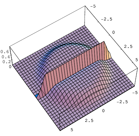
We see that the eigenvalues lie in a circle with radius of order $\sqrt{N}$ and that a finite fraction lies strictly on the real axis repelling the remaining pairs of complex conjugate eigenvalues from the real axis. Then we take the same set of eigenvalues and choose only that subset with one eigenvalue close to a fixed value $z_{2}$ . Plotting a histogram of this set we obtain $R_{2}(z_{1},z_{2})$ (Fig. 2).

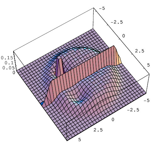
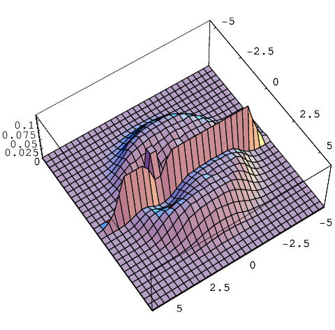
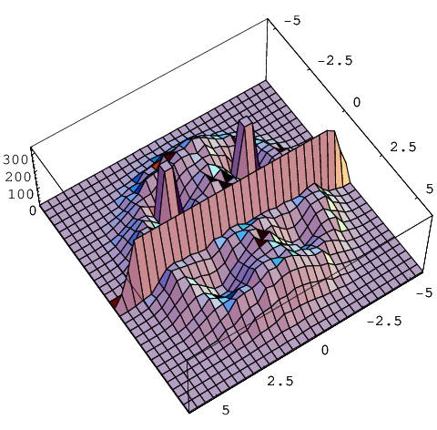
We see that the complex eigenvalue $z_{2}$ repells all the other with a cubic law in distance and that there is again a finite fraction of eigenvalues on the real axis corresponding to complex-real correlation. Furthermore one finds a $\delta$ -peak at the complex conjugate site $\overline{z_{2}}$ and also repulsion from that point. We can even take the same data, fix two eigenvalues $z_{2}$ and $z_{3}$ and plot $R_{3}(z_{1},z_{2},z_{3})$ as function of $z_{1}$ (Fig. 3).

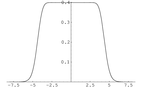
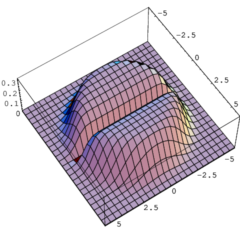
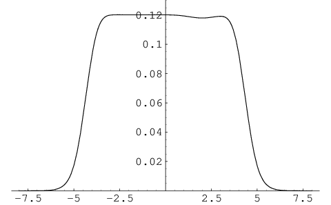
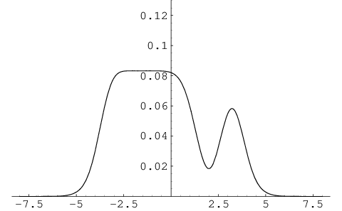
Using the above formulae we can calculate $R_{1}^{C}(1)$ , $R_{1}^{R}(1)$ , $R_{2}^{CC}(1,2)$ , $R_{2}^{RC}(1,2)$ , $R_{2}^{RR}(1,2)$ etc. exactly. Below we plot the functions $R^{R}_{1}(x_{1})$ , $R_{1}^{C}(z_{1})$ , $R_{2}^{RC}(x_{1},z_{2})$ and $R_{2}^{CC}(z_{1},z_{2})$ for the same fixed $z_{2}$ as in the simulation (Fig. 4-7).

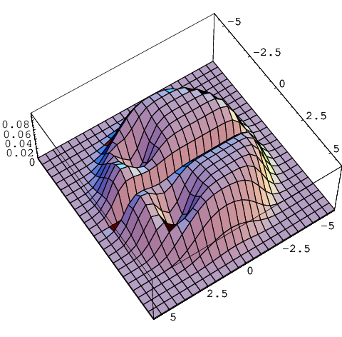
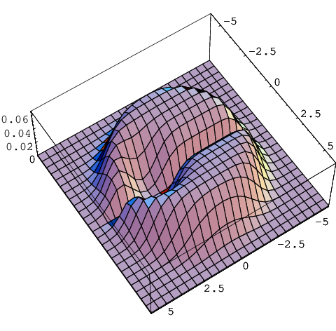
A further plot (Fig. 8) shows the correlation $R_{2}^{RR}(x,0)$ for $N=2,3,4,5,6$ , for which we have the analytical formula from eqs. (133, 127, 118, 125):

R_{2}^{RR}(x,0)=\frac{1}{\sqrt{2\pi}}R_{1}^{R}(x)-\frac{1}{2\pi}{\rm e}^{-x^{2}}+\frac{|x|}{2\sqrt{2\pi}}{\rm e}^{-x^{2}/2}\mbox{ erfc}(\frac{|x|}{\sqrt{2}})\,.

(134)

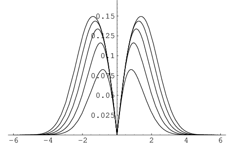
The only $N$ -dependence is in the first term $R_{1}^{R}(x)$ , which is almost constant in $x$ for sufficiently large $N$ . For small $|x|$ we have linear level repulsion. The connected correlation at the special point is independent of $N$ and decays with ${\rm e}^{-x^{2}}$ .

6 Conclusions

In this paper we have derived, starting from the Gaussian ensemble, closed analytical expressions for all correlation functions, i.e. $n$ -point densities, of eigenvalues of the real Ginibre ensemble of real asymmetric matrices, which is invariant under real orthogonal transformations. These $n$ -point densities are not absolutely continuous. They contain contributions which are concentrated by $\delta$ -functions on the real axis and also point-measures for pairs of complex conjugate eigenvalues which are always present, because the eigenvalues of a real asymmetric matrix are either real or pairwise complex conjugate. The $n$ -point densities are written as quaternion determinants of certain $2n\times 2n$ selfdual matrices, or as Pfaffians of corresponding skew-symmetric matrices. The Pfaffians can be derived from a zero-dimensional fermion field theory, similar in structure as the matrix Green functions in the Nambu space for superconductivity. All the $n$ -point densities are expressible in terms of a skew-symmetric measure ${\cal F}(z_{1},z_{2})$ containing one part concentrated on the complex conjugate pairs $z_{1}=\overline{z_{2}}$ and one part on the real eigenvalues $z_{1}=\overline{z_{1}}$ , $z_{2}=\overline{z_{2}}$ . For the $N$ -dimensional matrix $J_{ij}$ one constructs from ${\cal F}(z_{1},z_{2})$ a skew-symmetric kernel ${\cal K}_{N}(z_{1},z_{2})$ which together with ${\cal F}(z_{1},z_{2})$ yields the building blocks for the correlations.
To calculate ${\cal K}_{N}(z_{1},z_{2})$ one has to invert an $N\times N$ antisymmetric matrix $A_{kl}$ related to ${\cal F}(z_{1},z_{2})$ , which looks complicated, which however turns out to yield a very simple tridiagonal structure for $A^{-1}_{kl}$ . To find this it is enough to compare the Edelman result for the complex 1-point density with the general form of the 1-point density. This is sufficient to obtain all correlations in the case of even dimension $N$ . In the case of odd dimension $N$ one has to increase the dimension artificially by 1 and has to invert instead the $(N+1)\times(N+1)$ dimensional skew-symmetric matrix $B_{nm}$ . Again a simple argument using the result of Edelman, Kostlan and Shub for the real 1-point density reveals that $B^{-1}_{nm}$ has again a simple tridiagonal (but slightly more complicated) structure. In this paper we do not discuss detailed asymptotics for large $N$ , which has partly been discussed elsewhere [1, 8, 9] and which follows essentially from the asymptotic kernel ${\cal K}_{N}(z_{1},z_{2})\backsimeq(z_{1}-z_{2}){\rm e}^{+z_{1}z_{2}}/2\sqrt{2\pi}$ . However we show that the different formulae of the correlation functions for even and odd $N$ can be combined always in one formula which depends on continuous and even analytic functions of $N$ .

Finally we have presented some numerical simulations which make clear the complicated structure of the correlations, for example the 2-point correlation. There is a smooth background of complex-complex correlations, then a point measure for a complex conjugate pair, a part with one $\delta$ -function concentrated on the real axis for complex-real correlations and a part corresponding to real-real correlations doubly concentrated on the real axis. In comparison we have shown also some numerical evaluations of the analytical formulae.

For the future there remain to be discussed more detailed asymptotics and more sophisticated functions like level spacings and distributions of extremal eigenvalues.

This project has been supported by the Sonderforschungsbereich/Transregio 12 of the Deutsche Forschungsgemeinschaft.

General Eigenvalue Correlations for the Real Ginibre Ensemble

Abstract

pacs

1 Introduction

2 Joint density of eigenvalues

2.1 Dimension $N=2$

2.2 General derivation

3 Generating functional

3.1 Definition

3.2 Vandermonde determinant

3.3 Real case

3.4 General case

3.5 $Z[f]$ as a Pfaffian

4 1-point density

4.1 Even $N$ , complex eigenvalues

4.2 Even $N$ , real eigenvalues

4.3 Odd $N$

5 Correlation functions

5.1 Diagram expansion

5.2 Correlation functions, $N$ even

5.3 Expansion of a Pfaffian

5.4 Correlation functions, $N$ odd

5.5 Explicit expressions

5.6 Numerical evaluation

6 Conclusions

References

References

General Eigenvalue Correlations for the Real Ginibre Ensemble

Abstract

pacs

1 Introduction

2 Joint density of eigenvalues

2.1 Dimension N=2N=2

2.2 General derivation

3 Generating functional

3.1 Definition

3.2 Vandermonde determinant

3.3 Real case

3.4 General case

3.5 Z⁡[f]Z[f] as a Pfaffian

4 1-point density

4.1 Even NN, complex eigenvalues

4.2 Even NN, real eigenvalues

4.3 Odd NN

5 Correlation functions

5.1 Diagram expansion

5.2 Correlation functions, NN even

5.3 Expansion of a Pfaffian

5.4 Correlation functions, NN odd

5.5 Explicit expressions

5.6 Numerical evaluation

6 Conclusions

References

References

2.1 Dimension $N=2$

3.5 $Z[f]$ as a Pfaffian

4.1 Even $N$ , complex eigenvalues

4.2 Even $N$ , real eigenvalues

4.3 Odd $N$

5.2 Correlation functions, $N$ even

5.4 Correlation functions, $N$ odd

References

- [1] H.-J. Sommers, J. Phys. A 40, 671 (2007)
- [2] J.Ginibre, J. Math. Phys. 6, 440 (1965)
- [3] N.Lehmann and H.-J. Sommers, Phys. Rev. Lett. 67, 941 (1991)
- [4] A.Edelman, J. Multivariate Anal. 60, 203 (1997)
- [5] A.Edelman, E.Kostlan and M.Shub, J. Amer. Math. Soc. 7, 247 (1994)
- [6] G. Akemann and E.Kanzieper, J. Stat. Phys. 129, 1159 (2007)
- [7] C.D.Sinclair, arXiv: math-ph/0605006 (2006)
- [8] P.J.Forrester and T. Nagao, Phys. Rev. Lett. 99 050603 (2007)
- [9] A.Borodin, C.D.Sinclair, arXiv: math-ph/0706.2670v2
- [10] R.M.May, Nature 298 413 (1972)
- [11] H.Sompolinsky, A.Crisanti and H.-J.Sommers, Phys. Rev. Lett. 61 259 (1988)
- [12] K.B.Efetov, Phys. Rev. Lett. 79 491 (1997)
- [13] J.Kwapien, S. Drozdz, A.Z. Gorski and F. Oswiecimka, Acta Phys. Pol. B37, 3039 (2006)
- [14] W.Bruzda, V.Cappelini, H.-J.Sommers, K.Życzkowski, arXiv: quant-ph/0804.2361