Microscopic approaches for nuclear Many-Body dynamics
Applications to nuclear
reactions
ABSTRACT
These lecture notes are addressed to PhD student and/or researchers who want a general overview of microscopic approaches based on mean-field and applied to nuclear dynamics. Our goal is to provide a good description of low energy heavy-ion collisions. We present both formal aspects and practical applications of the time-dependent Hartree-Fock (TDHF) theory. The TDHF approach gives a mean field dynamics of the system under the assumption that particles evolve independently in their self-consistent average field. As an example, we study the fusion of both spherical and deformed nuclei with TDHF. We also focus on nucleon transfer which may occur between nuclei below the barrier. These studies allow us to specify the range of applications of TDHF in one hand, and, on the other hand, its intrinsic limitations: absence of tunneling below the Coulomb barrier, missing dissipative effects and/or quantum fluctuations. Time-dependent mean-field theories should be improved to properly account for these effects. Several approaches, generically named ”beyond TDHF” are presented which account for instance for pairing and/or direct nucleon-nucleon collisions. Finally we discuss recent progresses in exact ab-initio methods based on the stochastic mean-field concept.
I Introduction
I.1 General considerations
Heavy-Ion accelerators have given important information on nuclear reactions with stable nuclei. More and more precise measurements shed light on the interplay between reaction mechanisms and the internal structure of the two reaction partners. This interplay is perfectly illustrated by low energy reactions like fusion. For instance, fusion cross sections are influenced by vibrational and rotational modes of the nuclei [40]. New radioactive low energy beams facilities such as SPIRAL2, open new opportunities for these studies. Theoretically, microscopic models which incorporate both dynamical effects and nuclear structure in a common formalism should be developed. Dynamical theories based on the mean-field concept are of the best candidates.
The present lecture notes give a summary of actual progress in mean-field transport models dedicated to Heavy-Ion reactions at low energy. The starting point of different approaches, i.e. Time-Dependent Hartree-Fock with effective interaction, is described extensively in section II, while examples of applications are given in section III. TDHF should be extended to describe the richness of phenomena occurring in nuclear systems. In section IV, we introduce transport theories that incorporate effects such as pairing correlations and/or direct nucleon-nucleon collisions.
This lecture can be read at different levels. The reader interested in applications (section III) can skip most of the formal aspects described in section II. Section IV is relatively technical and requires a good understanding of the formal aspects described in section II. Finally, minimal notion of second quantization which are used in these notes are summarized in appendix A.
I.2 Microscopic Non-relativistic approaches
Typical examples of quantum microscopic theories used to describe static properties of atomic nuclei are: various Shell Models, mean-field and beyond theories (Hartree-Fock-Bogoliubov, Random-Phase-Approximation, Generator-Coordinate-Method…) [93] or algebraic approaches like the Interactive-Boson-Model [56].
Why should we also develop quantum microscopic approaches to describe nuclear reactions?
-
By itself, the N-body dynamical problem is a challenging subject.
-
Most of the information one could get from nuclei are deduced from nuclear reactions. Therefore a good understanding of the reaction is mandatory.
-
As already mentioned, it is necessary to develop a common formalism for both static and dynamical properties.
-
Microscopic theories have only few adjustable parameters (essentially the effective interaction), and we do expect that the predicting power is accordingly increased compared to more phenomenological approaches.
-
On opposite to most of macroscopic approaches which are specifically dedicated to a given mechanism, all dynamical effects should be ”a priori” included. For instance, TDHF can be used either to study reactions between two nuclei or collective motion in a single nucleus.
-
Using microscopic theories, we also expect to be able to deduce dynamical information on the behaviour of nucleons in the nuclear medium like for instance in-medium nucleon-nucleon cross sections
Last, microscopic approaches that will be described here are non relativistic. Relativistic effects are not expected to affect atomic nuclei because the typical velocities of nucleons are much less than the light speed .
I.3 What means independent particles?
It is relatively common to use words like ”mean-field theories” or ”independent particles systems” as well as their complement ”beyond mean-field” or ”correlated states”. Let us start with a discussion on this terminology. Then, we will be able to define the starting point of most of microscopic approaches dedicated to the description of nuclei.
I.3.1 Independent and correlated particles
We first assume two identical free fermions, one in a state and the other one in a state . Except for the Pauli principle which forbids , the fact that one fermion occupies is independent from the fact that the other occupies . We say that the two particles are ”independent”. The state vector associated to the two particles system accounts for anti-symmetrization and reads . Such a state is indifferently called independent particle state or Slater determinant (see appendix A). The concept of independence could be easily generalized to particles. A system will be called here ”independent particle system” if it could be written in a specific basis as an anti-symmetric product of single-particle states. In second quantization form (appendix A), such a state writes
| (1) |
On the opposite, we call ”correlated” a state that cannot be written in terms of a single Slater determinant, i.e. where each gives the probability of each configuration. Let us for instance consider a state describing two particles that decomposes onto two Slater determinants, i.e. . Then the concept of correlation becomes obvious because the occupation of one specific state affects the occupation probability of the other state. In this particular example:
-
If one particle is in the state , then the other is in .
-
If one particle is in the state , then the other is in .
I.3.2 Mean-field approximation
The aim of nuclear mean-field theories is to describe self-bound nuclei in their intrinsic frame where wave-functions are localized (on opposite to the laboratory frame). A possible description of a self-bound localized system in terms of Slater determinants could be constructed from single-particle wave-functions of an harmonic oscillator or a Woods-Saxon potential. These potentials are then interpreted as effective average mean-fields that simulate the interaction between particles. In other words ”Each nucleon freely evolves in a mean-field generated by the surrounding nucleons”. It is worth mentioning the necessity to consider intrinsic frame is very specific to self-bound systems like nuclei. For instance, for electronic systems, electrons are always considered in the laboratory frame since they are automatically localized due to the presence of atoms and/or external fields.
In this lecture, we consider more elaborated mean-field, generally ”called” self-consistent mean-field, like those found in Hartree-Fock (HF) and Hartree-Fock-Bogoliubov (HFB) theories. In the first case, the mean-field is calculated from occupied single-particles while the second case is more elaborated and requires the notion of quasi-particles (see section IV.1). In section II.2, TDHF equations are obtained by neglecting correlations. Last, although it is not the subject of the present lecture, it is worth mentioning that the introduction of effective interactions for nuclear mean-field theories leads to a discussion on correlation much more complex than presented here (see [103] for a recent review).
I.3.3 Mean-free path and justification of mean-field approaches in nuclear physics
Can independent particles approximation give a good description of nuclear systems including reactions between two nuclei? The justification of mean-field theories is largely based on the empirical observation that many properties vary smoothly for nuclei along the nuclear charts: single-particle densities, energies… Based on this consideration, macroscopic and mean-field models have been introduced and turns out to be very successful to describe nuclei. Therefore, by itself, the predicting power of independent particle approximation justify a posteriori its introduction.
The large mean-free path of a nucleon in nuclear matter (larger than the size of the nucleus itself) gives another justification of the independent particle hypothesis [20]. This implies that a nucleon rarely encounter direct nucleon-nucleon collision and can be, in a good approximation, considered as free. This might appear surprising in view of the strong interaction between nucleons but could be understood as a medium effect due to Pauli principle. Indeed, the phase-space accessible to nucleon after a direct nucleon-nucleon collision inside the nucleus is considerably reduced due to the presence of other surrounding nucleons (essentially all states below the Fermi momentum are occupied). However, if the relative kinetic energies of two nucleons increases, which happens when the beam energy increases, the Pauli principle become less effective to block such a collision and the independent particle approximation breaks down.
I.3.4 Symmetries and correlations
Small remarks against the intuition: independent particle states used for nuclear systems contain correlations. This could be traced back to the fact that some symmetries of the original Hamiltonian are generally broken. For instance, nucleons described within the nuclear mean-field approach are spatially correlated because they are localized in space. This is possible because mean-field is introduced in the intrinsic frame and translational invariance is explicitely broken. Indeed, if we do not break this symmetry, then the only mean-field solution would be a constant potential and associated wave-functions would be plane waves. We then come back to the free particle problem which are not self-bound anymore.
We illustrate here an important technique which consists in breaking explicitly symmetries to incorporate correlations which could hardly be grasped in an independent particle picture (see for instance [13]). Among the most standard symmetries explicitly broken generally to describe nuclear structure, we can quote breaking of rotational invariance which authorizes to have deformed nuclei and help to recover some long range correlations11 1 Let us consider an elongated nucleus (”cigare” shape), the fact that one nucleon is at one side of the cigare implies necessarily that other nucleons should be on the other side. This should be seen as long range correlations that affects nucleons as a whole.. Gauge invariance (associated to particle number conservation) is also explicitly broken in HFB theories in order to include short range correlations like pairing (see section IV.1). The latter approach will still be called ”mean-field”. It however goes beyond independent particle approximations by considering more general Many-body states formed of product of independent quasi-particles (a summary of terminology and approximations considered here is given in table 1).
I.3.5 Theories beyond mean-field
In nuclear physics, mean-field is often considered as the ”zero” order microscopic approximation. Many extensions are possible (several ”beyond mean-field” approximations will be presented in section IV). These extensions are generally useful to include correlations that are neglected at the mean-field level. As we will see, ”beyond mean-field” approximation are absolutely necessary to describe the richness of effects in nuclear structure as well as in nuclear dynamics. In particular, not all correlations could be incorporated by only breaking symmetries and often one has to consider the state of the system as a superposition of many independent (quasi)particles states.
The previous discussion clearly points out that mean-field approaches might include correlations. Nevertheless, the terminology that is generally used (and that we continue to use here) is that non-correlated state will be reserved to Slater determinant states. A correlated state then refers to a superposition of Slater determinants. Table 1 summarizes different approaches that will be discussed in this lecture and associated type of correlations included in each approach.
| Name | Approximation | Variational space | Associated observables |
|---|---|---|---|
| TDHF | mean-field | indep. part | one-body |
| TDHF-Bogoliubov | m.-f. + pairing | indep. quasipart. | generalized one-body |
| Extended-TDHF | m.-f. + collision (dissipation) | correlated states | one-body |
| Stochastic-TDHF | m.-f. + collision | correlated states | one-body |
| (dissipation+fluctuations) | |||
| Time Dependent Density Matrix | c.m. + two-body correlations | correlated states | one- and two-body |
| Stochastic Mean Field | Exact (within statistical errors) | correlated states | all |
| (Functional integrals) |
I.4 Effective interaction and Energy Density Functional (EDF)
We will use in the following a rather standard approach to the nuclear many-body problem. Starting from a microscopic two-body Hamiltonian and using second quantization, we introduce the Hartree-Fock theory. It is however worth mentioning that the use of most recent realistic two-body (and normally three-body) interactions will not lead to reasonable results (if any) at the Hartree-Fock level. In view of this difficulty, the introduction of effective interactions adjusted to nuclear properties was a major break-down. These interactions are not directly connected to the original bare interaction and are expected to include effects (in particular in-medium effects) that are much more involved than in the standard Hartree-Fock theory. In that sense, mean-field theories in nuclear physics have many common aspects with Density Functional Theories (DFT) in condensed matter. However, in nuclear physics we often keep the concept of effective interactions.
The most widely used interactions are contact interactions (Skyrme type) and finite range interactions (Gogny type). The second type of interactions is still too demanding numerically to perform time-dependent calculations and only Skyrme forces are nowadays used for TDHF. To relax some of the constraints due to the use of effective interactions, the more general concept of Energy Density Functional (EDF) is introduced. In that case, the static and dynamical properties of the system are directly obtained by minimizing a functional of the one-body density, denoted by [45, 14].
I.5 The N-body problem: basic formalism
The evolution of a Many-Body state is given by the time-dependent Schrödinger equation
| (2) |
This equation can equivalently be formulated in term of a variational principle. In that case, the quantum action is minimized between two times and with respect to the wave-function variations
| (3) |
The Many-body Hamiltonian decomposes into a kinetic term and a two-body interaction term (for the sake of simplicity, we will not consider higher order interactions)
| (4) |
In second quantization (appendix A), the Hamiltonian writes
| (5) |
where matrix elements associated to the kinetic energy and anti-symmetric two-body interaction are given respectively by
| (6) | |||||
| (7) | |||||
| (8) |
Note that here, the two-body state is not anti-symmetric. This notation means that the particle ”1” is in the state , while the particle ”2” is in the state (for further details on notations see appendix A).
Let us again summarize the overall goal: Even if we were able to solve the exact Many-Body problem (Eq. (2)), which is not the case anyway in nuclear physics, we do not need to have all the information contained in the exact wave-function to understand physical processes related mainly to one-body degrees of freedom, like collective motion or fusion reactions. Construction of microscopic models are therefore guided by two principles:
-
we focus exclusively on what we really need,
-
we do relevant approximations for the considered problem.
A strategy of approximation consists in focusing on specific degrees of freedom. This is generally equivalent to minimize the variational principle (3) on a restricted subspace of the total Hilbert space of Many-body wave functions [16]. The selection of this subspace is crucial and is driven by the physical process considered.
Among the microscopic transport theories, the TDHF method, proposed by Dirac in 1930 [43] as an extension of the Hartree-Fock static mean-field theory [53, 47] is a tool of choice. It corresponds to a mean-field theory where the only input is the effective two-body interaction. In practice, TDHF Equations can be derived by restricting the variational space to Slater determinants.
In the following, formal and practical aspects of TDHF are presented. Then examples of applications to reactions close to the fusion barrier are given. Successes and limitations of TDHF will illustrate physical effects missing in this approximation. ”Beyond mean-field” theories that incorporate these effects are finally discussed.
II Dynamical mean-field theories
Let us recall the two basic questions:
-
What is the relevant information for the description of nuclear reactions ?
-
What approximations can (and cannot) be done to treat this information ?
The knowledge of nuclei trajectories during collisions, their shapes or particle numbers already gives a good understanding of the reaction mechanisms. All these quantities are related to one-body degrees of freedom (see appendix B). Therefore, if we are able to give a realistic description of the one-body density matrix, we will also correctly reproduce these observables. As we will see, the reduction of the information to one-body degrees of freedom is intimately connected to the independent particle approximation discussed in the introduction. This will answer the second question. Starting from the Schrödinger equation, the equation of motion for the one-body degrees of freedom (contained in the evolution of the one-body density) is obtained. Then connections with the independent particle approximation are discussed. Finally, we describe practical aspects related to the resolution of TDHF.
Readers not interested in formal details can jump to Eq. (34) which gives the most general form of the one-body density evolution for any Many-Body system.
II.1 Expectation values of one-body observables
II.1.1 General expression
Let us consider a system of particles (eventually correlated) and a one-body operator (see Eq. (174)). Starting from general expression of a Many-Body wave-function (Eq. (161)) and using the closure relation (Eq. (173)), we obtain
| (9) | |||||
where spin and isospin quantum numbers are included in the notation . Using the Wick’s theorem (see appendix A.3), leads to
| (10) |
Using the anti-symmetry of each state of the basis, it is possible to reduce, in integral (9), the action of to the first label ”1” only. Noting the matrix elements of , we obtain
| (11) |
II.1.2 One-body density matrix
We introduce the one-body density matrix associated to the state . Its matrix elements in the basis are given by
| (12) |
Accordingly, equation (11) can be simply expressed as
| (13) |
Therefore, all the information required to estimate a one-body observable is contained in the one-body density matrix. Such a matrix can always be associated to any system of particles22 2 It is worth mentioning that the discussion presented here can be generalized to -body observables. In that case, we can define the -body density that contains all the information on -body (and below) quantities (see appendix C).. In the following, we will essentially consider properties of the one-body density and omit exponent (1).
Using second quantization, matrix elements of are defined as (see Eq. (180))
| (14) |
Eq. (12) can indeed be recovered using (154), (161) and (173)
| (15) | |||||
In the following, the one-body density components are introduced in a specific single-particle basis. For instance (see section II.4), TDHF calculations are often performed in coordinate representation. In that case, using equations (142) and (143), we have
| (16) |
where single-particle wave-functions are defined in Eq. (137).
Note that, we can always write the one-body density matrix as an operator acting in the Hilbert space of the single-particle wave-functions33 3 This definition of operators should not be confused with the definition of one-body operators given in appendix B since it is not defined in the space of many-body wave function. [93]
| (17) |
In particular, this operator depends on the system wave-function and then it is a funtion of the time during a collision.
Let us come back to one-body observables. The second quantization simplifies the calculation of their expectation values. Using Eq. (175), we have directly
| (18) |
which is nothing but Eq. (13). Therefore we see that the evolution of any one-body observable can be obtained from the evolution of the one-body density matrix.
II.1.3 The independent particle case
Let us consider the case of a system described by a Slater determinant . The associated one-body density is denoted by . In appendix E, we show that any Slater can be considered as a vacuum (called HF vacuum) for specific operators written as linear combination of the and . We can thus apply the Wick’s theorem. Methodology associated to the Wick’s theorem as well as contractions are given in appendix F. This technique (Eq. (196)) implies that only occupied states contribute to the summation in Eq. (16). We finally end with
| (19) |
Therefore, for Slater determinants, the knowledge of occupied states is equivalent to the knowledge of one-body density matrix. The specificity of independent particles systems is that all the information is contained in the one-body density. This is nicely illustrated by the fact that any -body density matrix could be expressed as an anti-symmetric product of one-body densities leading to vanishing -body correlation matrices at all orders (see appendix C).
For dynamical problems where the Many-Body state is assumed to stay in an independent particle state at all times (this is the case of TDHF presented in section II.2), it is sufficient to only follow the one-body density in time. This is strictly equivalent to follow occupied states.
Note finally the following useful property: for an independent particle state, . Indeed, the operator given by Eq. (17) then writes
| (20) |
Therefore, is nothing but the projector on the subspace of occupied single-particle states of . Considering a set of orthonormal single-particle states, we have
| (21) |
Assuming the above relation for the one-body density is equivalent to assume independent particle states.
II.1.4 Dynamical Evolution from the Erhenfest theorem
As discussed above, the basic approximation is to focus on a specific class of observables, which are the one-body observables in our case. Considering any observable , using (Eq. (2)) and its Hermitian conjugate for any N-body state , we have
| (22) |
which is nothing but the standard Ehrenfest theorem for the operator . The above equation is exact and valid for any (correlated or not) state and observable. Here, is the full microscopic Hamiltonian (see Eqs. (4) and (5)). For a one-body operator, can be written as a linear combination of the . Therefore, it is sufficient to follow the expectation values of the , which are nothing but the matrix elements of and are given by
| (23) |
II.2 Time-Dependent Hartree-Fock (TDHF)
II.2.1 Exact evolution of
Our goal is to provide the best description as possible of the one-body density matrix evolution. The only approximation that will be made is that the system remains in an independent particle state at all time. Several derivations of TDHF exist so far. Here, we use the Ehrenfest theorem as a starting point.
Reporting the Hamiltonian expression (Eq. (5)) in the evolution of the (Eq. (23)), we get
| (24) |
Let us start with the first term associated to kinetic energy. Using Eqs. (140) and (141), we obtain
| (25) | |||||
The kinetic energy term reduces to
| (26) |
For the two-body interaction, we should first express the expectation value of the commutator
The two terms with 6 annihilation/creation operators cancel out. Other terms are nothing but components of the two-body density matrix (defined in appendix C). The two-body density can be decomposed into a sum of an anti-symmetric product of two one-body density (the uncorrelated part) plus the so-called two-body correlation matrix, denoted by (see appendix D). Using this decomposition (Eq. (183)), Eq. () writes
where exponents (1) and (2) in equation (183) have been omitted for simplicity. Altogether, the two-body interaction contribution to the one-body evolution reduces to
| (29) | |||||
where we have used and the anti-symmetry of 44 4 The fact that is anti-symmetric is a consequence of the anti-symmetry of and can be deduced from anti-commutation rules for fermions (140) entering in the definition of (Eq. (180)).. The two-body contribution can finally be written as
| (30) |
where is the Hartree-Fock self-consistent mean-field. The latter can be written with the use of partial traces as
| (31) |
The trace is only made on the second particle ”2” while the labels and correspond to the particle labeled by ”1”. The matrix therefore corresponds to a one-body mean-field operator. In the following, we will often use the notation and . Then, Eq. (31) simply reads .
The second term in equation (30) reflects the effect of correlations on the evolution of one-body degrees of freedom. It can also be written with a partial trace on the particle ”2”
| (32) |
Then, using Eqs. (14), (24), (26), (30) and (32) we finally deduce that the most general expression of the one-body density for any correlated system with a two-body interaction can be written as
| (33) | |||||
The anti-symmetry of and implies that and finally leads to the more compact form
| (34) |
where
| (35) |
is the matrix associated to the one-body Hartree-Fock Hamiltonian. Note that, up to here, since no approximation has been made, the dynamical evolution of the one-body density is exact. However, the equation above requires a priori to also follow the two-body correlations in time which may be to complicated.
II.2.2 Time-dependent mean-field approximation
In TDHF, two-body correlations are neglected at all time, i.e. .This is equivalent to assume that the system remains in an independent particle state at all time (see appendix F). Starting from Eq. (34) and neglecting the correlation term, we finally get the TDHF equation for the one-body density matrix
| (36) |
In this section, we will now concentrate on the latter equation which could also be written in terms of operators as
| (37) |
where and act both on the Hilbert space of single-particle states. In a complete basis of this space with the closure relation , we have
| (38) |
Let us now give some properties of equation (37). First is preserved. Therefore at all time, the density could be decomposed on a set of single-particle states (Eq. (20)). The TDHF equation can equivalently be written in terms of coupled self-consistent equations on the single-particle states
| (39) |
Indeed, starting from the expression of and using the above Schrödinger-like equation for single-particle states, we recover the TDHF equation (Eq. (37)) that
This shows the equivalence of the single-particle representation and density formulation.
Though Eqs (39) take the form of Schrödinger equations, they are non llinear because the Hamiltonian depends on the one-body density. As a consequence it depends explicitly on time. We clearly see here some difficulties of mean-field theories. Indeed, we want to describe the system evolution between the initial and final time with a Hamiltonian which is itself depending on the evolution.
II.3 The Skyrme effective interaction
Mean-field equations have been derived for any general two-body Hamiltonian. However, in practice, the interaction is chosen to simplify numerical aspects. Most (if not all) applications of TDHF in the nuclear context have been performed using the Skyrme like [102] interaction. The most widely used Skyrme force writes
| (40) | |||||
where , (relative impulsion), , , , are operators acting on the spin of particle and are given in terms of Pauli matrices acting on the spin space. corresponds to the exchange of the spin. is the particle density at . ”” and ”” terms are non-local in space and simulate the short range part of the interaction. Finally ”” is the spin-orbit term.
The very interesting aspect of this interaction is its zero range nature, which greatly simplifies the mean-field expression in coordinate space. Parameters (, , and ) are generally adjusted to reproduce nuclear properties like saturation, incompressibility … of nuclear matter and selected properties of finite nuclei (see for instance [34, 35, 79]).
An important aspect of the fitting procedure which has direct implication on nuclear reactions calculations is the following: for nuclear structure calculation, center of mass contribution are removed (see section 3.2. of ref. [35]) to obtain a better description of nuclei in their intrinsic frame. For collisions, only the intrinsic frame of the total system is considered and the same correction used for a single nucleus could not be used anymore. This is the reason why specific forces which explicitly do not account for center of mass correction have been developed like SLy4 [60] where parameters of the force have been adjusted to reproduce the same properties as Sly4 [35] except that the center of mass correction is neglected.
Note finally that the ”” term in Eq. (40) explicitly depends on the system density. For specific integer values of , the density dependent two-body interaction could be interpreted as a higher order interaction. In practice, non-integer values of turns out to be more effective in reproducing nuclear properties. This however has important consequences. In particular, since the interaction depends on the system on which it is applied, strictly speaking, we cannot really use the terminology ”interaction”. One often use the very notion of Energy Density Functional to avoid confusion. In addition, translational invariance (but not Galilean invariance [106]) is explicitly broken.
II.4 Numerical implementation of TDHF: practical aspects
Several applications of TDHF have been performed in the last decade for nuclear collective motion studies [97, 82, 3, 112, 91, 92] and nuclear reactions [60, 96, 98, 113, 77, 114, 115, 116, 50, 117, 99, 100, 51, 118] with various numerical methods to solve the TDHF equation. We present here a method used to implement TDHF for nuclear collisions. Different steps of a calculation are presented to better illustrate numerical constraints. To apply TDHF, we should
-
Construct the HF ground states of each of the collision partners. This requires to first solve their HF equations.
-
Starting from two Slaters at an initial distance , one should construct a single Slater associated to the composite system.
-
The nuclei should be initially positioned and boosted to properly account for the reaction properties (Beam Energy, impact parameter…)
-
The dynamical evolution should be performed iteratively to solve the self-consistent TDHF equations. This is generally done by solving the Time Dependent Schrödinger equations on occupied states.
-
Finally, we should compute a set of observables to get informations on the reaction itself.
Since all the information is contained in the one-body density, only one-body wave-function need to be considered.
Sections II.4.1 to II.4.4 describe respectively the construction of initial Slater determinants and how initial conditions for reactions according to Rutherford trajectories are imposed. Section II.4.5 presents the numerical implementation of mean-field transport equations.
II.4.1 Hartree-Fock initial state
We assume that the collision partners are initially in their ground states. Consistently with the TDHF approach, we should consider that the ground state of both nuclei are solution of the self-consistent Hartree-Fock (HF) states. The one-body density associated to each state is solution to the stationary version of the TDHF equation (Eq. (37)):
| (41) |
This equation is valid in any basis. Then, a specific basis should be chosen to explicitly solve the equation. Since and do commute, we can choose common eigenstates. We denote this basis by with and . Here occupation numbers verifies ou 1. The -body Slater determinant state is constructed from the occupied states (with ).
Eigenvalues of can eventually be interpreted as single-particle energies [119]. In the HF approximation, the ground state is obtained by filling the lowest energy single-particle states. Therefore, we only need to find the lowest eigenstates of .
II.4.2 Imaginary-time method
The imaginary-time method [41] is a widely used method to find the lowest eigenvalues of an operator (whose eigenstates is bound from below). Let us illustrate this method for a particle in an external field. The method consists in starting from an initial wave-function which is not a priori an eigenstate of the one-body Hamiltonian, denoted by . This state can be decomposed onto the true eigenstates ()
| (42) |
We apply the operator on the initial state
| (43) |
The lowest energy eigenstate associated to can then be obtained from
| (44) |
Indeed, we have and then for except for , only the ground state component does not vanish. The denominator is required because is not unitary (). The terminology ”Imaginary-time” comes obvisouly from the fact that looks like the propagator in time where the time is a complex quantity . It is finally worth to mention that the initial state should be guessed in order to contain at least a small fraction of the lowest eigenstate.
The imaginary-time method should be further improved to obtained eigenstates of the single-particle HF energies. Indeed, two additional difficulties exist:
-
Since the system is composed of particles, we need the lowest eigenstates of and therefore we need to guess initial starting points for the single-particle wave-functions.
-
The Hamiltonian is non-linear and depends explicitly on the system density .
To solve the first difficulty, we apply the imaginary time method imposing that the states remain orthonormal (through a Graham-Schmidt orthogonalization for instance). We then expect to converge towards the lowest eigenstates if the states are not initially orthogonal to the ”true” eigenstates. A common choice for the initial states are those of Harmonic or Nilsson potentials.
To solve the second difficulty, we procede iteratively with small imaginary-time steps . At each step, the density is calculated from the states and the mean-field Hamiltonian is modified accordingly.
A schematic representation of the different steps of the imaginary-time procedure is
| (45) |
Here denotes the normalization of the state ”i”. Note that, ”” is an extra parameter generally used to slow down the convergence and avoid numerical instability [24]. In practice, it has the effect to mix the mean-field Hamiltonian at a step ”n” with the one at the step ”n-1”. The small time-step increment are generally performed using simple development of the exponential, i.e. . Again, since the latter is not unitary a Graham-Schmidt method is used at each iteration.
In practice, a specific Hilbert space basis should be first chosen to numerically express the different steps depicted in (45). The most common choice is either the space (resp. momentum) coordinate representation ( resp. ) or harmonic oscillator basis . In both cases, since an infinite number of states could not be considered, the basis has to be truncated. In coordinate case, this is achieved by restricting the space to a discrete finite box while in the Harmonic oscillator basis a limited number of major shells is considered. Once the basis is selected, all ingredients of the theory are expressed in this basis.
At the end of the iterative procedure, a set of single-particle states is obtained that completely defines the HF ground state. Unoccupied levels could also be obtained in a similar way although they do neither affect the density nor the mean-field. In Figure 1, individual densities associated to neutron states in 16O and obtained with the imaginary-time method are presented. In that specific case, the discretized coordinate space was used. Technically, the box should be taken sufficient large to avoid the effect of the boundary. Here Hard Boundary conditions are retained imposing that wave-functions cancel out outside the box. Note finally, that in Fig. 1, only the , and single-particle states are occupied 55 5 Each state presented here is doubly degenerated due to the explicit assumption of time-reversal invariance in the calculation..

II.4.3 The two nuclei case: initial state construction
Since each nucleus has been constructed in its HF ground state, we start from two independent particles systems to construct the initial TDHF condition. However, we have shown previously that Eq. (36) describes a priori the evolution of a single Slater determinant.
It is however always possible to construct a Slater determinant associated to independent particles from two Slater determinants and if the two systems are initially well separated. Let us consider the two one-body densities and . For each densities we have (see section II.1.3). If we now construct the square of the total density
| (46) |
where H.c. stands for Hermitian conjugated. Therefore, to have , single-particle states should not overlap. In practice, this is possible due to ”Hard boundary” conditions in the HF calculations which impose that the single-particle wave-functions vanish at some distance. Therefore, we should just be careful to consider a box for TDHF that is large enough to avoid overlap between the two boxes used in the HF case (see figure 2).

II.4.4 Dynamical evolution of nuclei
The TDHF theory is a quantum theory since it treats explicitly the particles with wave-function. However, the restriction to independent particles states does not allow, in general, for a probabilistic interpretation of reactions channels. Accordingly, some quantum aspects are missing, we will clearly see this pathology in fusion reactions (where the fusion probability will either be 0 or 1). Essentially, TDHF gives classical trajectories for the evolution of centers of mass.
We consider the system in its total center of mass frame. The impact parameter and beam energy (which fixes the initial velocity of the projectile at infinite distance) allow us to determine the initial TDHF condition. At this initial time (), the two nuclei have a relative distance . In general, a Rutherford trajectory is assumed to account for Coulomb trajectory from infinity to . This hypothesis is consistent with the assumption that the two nuclei are in their ground state at , i.e. we assume that no energy has been transfered from the relative motion to internal degrees of freedom up to .
Using notations of section II.4.3, a velocity is applied to each nucleus ( or 2) imposing the impulsion . This is performed, by applying a translation of each in momentum space [106]
| (47) |
where the position operator acts in single-particle space. Note that, here is reserved to the static HF while with time in parenthesis corresponds to boosted HF.
In practice, since one usually follows directly single-particle wave-functions, the translation in momentum space is directly applied to the waves
| (48) |
Once the two nuclei are positioned on the network and properly boosted, there is no more reason to distinguish single-particle states from one or the other collision partner.
II.4.5 Numerical methods for dynamics
To solve the system of equations of motion, we should solve TDHF equations for occupied states (Eq. (39)). The main difficulty is the fact that the Hamiltonian itself depends on time. As a consequence, as in the imaginary-time case, specific procedure should be implemented to account for self-consistency in propagators. We consider a small time step increment and perform the time evolution iteratively. Over small time intervals , the Hamiltonian is almost constant. However, to conserve the total energy, the numerical algorithm should be symmetric with respect to time-reversal operation. This implies to consider the Hamiltonian value at time for the evolution of wave-functions from to [46] 66 6 This algorithm is similar to a Runge-Kutta method.
| (49) |
A schematic illustration of the real time propagation could be written as:
| (56) |
where corresponds to an approximation of . In this algorithm, starting from the density at time , a first estimate of the density at time , denoted by is obtained. The Hamiltonian used in the propagator is then computed using the average density obtained from and . Then, the real new density at time is obtained using this Hamiltonian. As in the imaginary-time case, an approximate form of the exponential is generally used which in some cases, breaks the unitarity (even in the real time evolution) and orthonormalization of the single particle states must be controlled.
III Application of TDHF to reactions around the fusion barrier
TDHF has been applied to nuclear physics more than thirty years ago. First applications were essentially dedicated to fusion reactions [21, 22, 46, 83]. Figure 3, adapted from P. Bonche et al. [22], illustrates the predicting power of TDHF for fusion cross sections. The main difference with actual calculations is that, at that time, several symmetries were used to make the calculation tractable. The major advantage of imposing symmetry was to reduce the dimensionality (and therefore the numerical effort). The major drawback was the reduction of applicability. The second difference with nowadays calculations comes from the fact that simplified forces were used, missing the richness of effective interactions used in up to date nuclear structure studies. Recently, all symmetry assumptions have been relaxed and forces using all terms of the energy functional have been implemented [113]. We present here several applications in 3D coordinate space with the full SLy4 [60] Skyrme force.
First, general aspects related to fusion reactions are presented, like fusion barrier properties, cross sections… Then, we illustrate how a microscopic dynamical model can be used to get informations from the underlying physical process. Besides fusion probability, transfer of nucleon will be discussed. Finally, limitations of standard mean-field models are discussed.

III.1 Selected aspects of fusion
III.1.1 Definition of fusion
Nuclear fusion is a physical process where two initially well separated nuclei collide and form a compound nucleus which has essentially lost the memory on entrance channel (Bohr hypothesis). This hypothesis is rather simple while the experimental measurement is rarely trivial. Indeed, energy and angular momentum conservations imply compound nucleus generally formed at rather high internal excitation and angular momentum. As a consequence, the fused system cools down by gamma, particle emissions and/or eventually fission. Overall, several decay channels are competing leading to a broad range of final phase-space which eventually overlaps with direct reactions (and more generally pre-equilibrium) processes. This is for instance the case of quasi-fission (where the systems keep partial memory of the entrance channel) which leads to mass and charge distribution which can eventually be similar to fission. Similarly complete and incomplete fusion are sometimes difficult to disentangle due to the presence of direct break-up channels (which are enhanced in the weakly bound nucleus case). Therefore, fusion events are sometimes experimentally difficult to distinguish from other processes.
III.1.2 One dimensional approximation
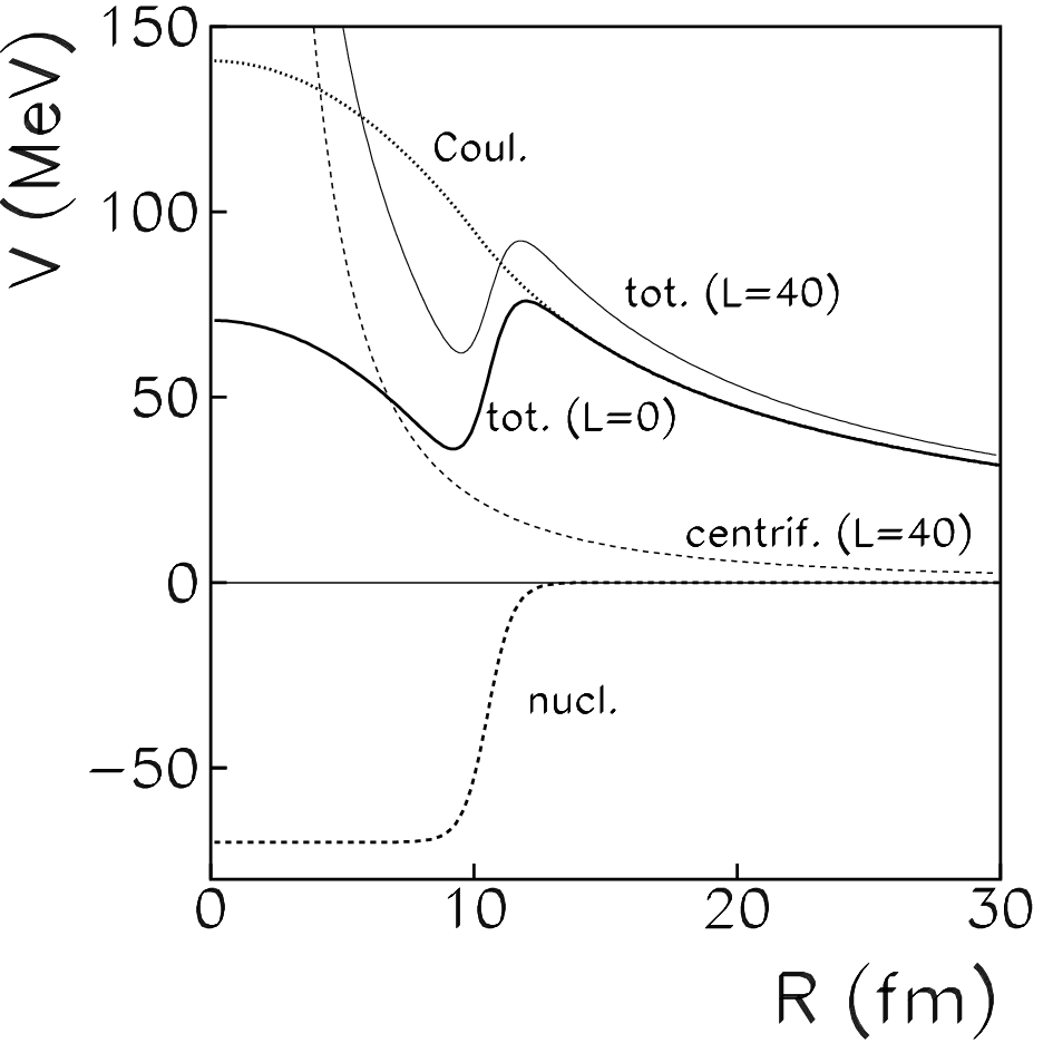
The simplest approach to fusion reaction is to consider the relative distance between the centers of mass of the nuclei as the most relevant degree of freedom. Fusion reactions then reduce to the dynamical evolution in a one-dimensional potential where the potential is deduced from the long-range Coulomb repulsive interaction of the two nuclei and from their short range mutual nuclear attraction (see figure 4). We assume that fusion takes place when the system reaches the inner part of the fusion barrier ( on figure 4).

Within this approximation, fusion cross sections can be expressed as a function of the transmission probability for each energy E and angular momentum
| (57) |
where denotes the reduced mass. Below the fusion barrier, i.e. , fusion is possible only by quantum tunneling. Using the WKB (Wentzel-Kramers-Brillouin) approximation leads to the following transmission coefficients
| (58) |
where is the total (nuclear + Coulomb + centrifugal) potentials while and correspond to ”turning points” at energies (see Fig. 4). Another simplification can eventually be made using a parabolic approximation. In that case, the potential is approximated by an inverted parabola with curvature . This approximation is justified close to the fusion barrier only and leads to analytical expression for the transmission coefficients
| (59) |
Finally, summation on different leads to the Wong formula [123]
| (60) |

Predictions of this one-dimensional approximation are compared to experimental observations for O+Sm and Ni+Ni systems in Fig. 5. The comparison is relatively satisfactory above the barrier but fails to reproduce sub-barrier cross-sections which are underestimated by several orders of magnitude by the Wong formula.
In addition, experimental data clearly show large differences from one isotope to the other which underlines the inherent nuclear structure effects and could not be simply explained by the change of the radii. Note finally that improvements where the parabola and/or the WKB approximations are not made do not improve significantly the comparison.
III.1.3 Coupling between relative motion and internal degrees of freedom
The discrepancy between experiments and simple estimates can directly be traced back to the fact that we assumed nuclei as rigid objects without internal structure. In fact, fusion is affected by the reorganization of internal degrees freedom as the two nuclei approach. This induces a coupling between the internal degrees of freedom and the relative motion. The only way to include this effect is to add additional degrees of freedom in the description of fusion. At the macroscopic level, this is generally achieved by introducing, for instance, deformation, orientation, neck parameters, mass and charge asymmetries leading to more complex ”multi-dimensional” potentials (see [67] and references therein). This will be illustrated with TDHF calculations below, in particular to study the effects of deformation.
Sub-barrier fusion is a perfect illustration of effects induced by couplings to internal degrees of freedom. These couplings can lead to an ensemble of fusion barriers called barriers distribution and can give enhancement of cross sections by several order of magnitude in the sub-barrier fusion regime77 7 Note that, as a counterpart, fusion above the barrier are usually reduced compared to the one-dimensional case.. A proper description of these effects could only be achieved if inelastic excitations, collective modes, transfer and all relevant processes are properly accounted for (see [8, 40]).
Note finally that additional important effects could appear when weakly bound nuclei are involved. In particular, break-up channels and new collective modes may become important. From an experimental point of view, influence of these new effects on reduction/increase of fusion cross sections is still under debate. With future low energy radioactive beams, we do expect to get additional informations on the reaction mechanisms with weakly bound nuclei around the barrier.
III.1.4 Barriers distribution
The experimental barriers distribution is obtained from the excitation function using the relation [94]
| (61) |
This function could be interpreted as the probability that the system has its barrier at energy .
Let us illustrate this with a simple cases. Consider a classical model with a single barrier at energy . In that case, identifies with the Dirac function . The latter formula is consistent with the fusion probability found in classical systems (i.e. ) deduced from the Wong formula (60). The fusion probability is zero below the barrier and equal to for . We therefore deduce that the distribution barrier reads which is the expected behavior. For quantum systems, spreads over a wider range of energies.
III.2 Fusion barriers and excitation functions with TDHF
III.2.1 Fragments trajectories
A way to characterize TDHF trajectories consists in matching the microscopic theory with the one-dimensional model described previously. The main difficulty is then to define the relative distance between the two nuclei. When fragments are well separated, such a distance could be easily defined. On the opposite, after the touching, this becomes more complicated and could only be achieved for short time after the touching. Fortunately, around the barrier, nuclei are generally still well separated. In practice, the main axis of the reaction could be extracted (it generally corresponds to the main axis of deformation) [121]. Then, along this axis, the local minimum of the density profile defines the separation plane (see figure 6). Note that this distance does not cancel out even for one sphere.

III.2.2 Barriers distribution for two initially spherical nuclei
We first consider 16O+208Pb reaction. The two nuclei are initially in their ground state and are at a relative distance fm. Evolutions of relative distances for head-on collisions ( fm) obtained from different center of mass energies (from 74.2 et 75 MeV) are displayed in Fig. 7 88 8 Each trajectory presented in figure 7 have been computed using 4 hour CPU time on a NEC/SX-8 processor.. Due to the narrow range of initial center of mass energies, relative distance evolutions before touching are all similar. On opposite, after fm/c, we clearly see two groups of trajectories:
-
MeV, the two fragments re-separate.
-
MeV, the relative distances remain small ( 10 fm).
The latter case corresponds to the formation of a compound nucleus after the collision. A precise analysis shows that the predicted fusion barrier lies between 74.44 and 74.45 MeV. Experimentally, it is found around 74 MeV, with a width of 4 MeV. It is rather interesting again to mention that TDHF seems to precisely describe fusion barrier while no parameters of the effective interaction has been adjusted on reactions.

In order to better understand phenomena occuring in TDHF around the fusion barrier, the local part of the one-body density () evolutions are displayed in Figs. 8 and 9 respectively for energies just below and above the estimated fusion barrier. In the former case, the composite system hesitates to fusion. It forms a ”di-nuclear” system for relatively long time ( fm/c) before re-separating. During this time, nucleons are exchanged between the two partners. In the second case, the system passes the fusion barrier (it is just 10 keV above the barrier). More generally, the two figures illustrates the richness of physical phenomena contained in TDHF: surface diffusivity, neck formation at early stage of fusion process, quadrupole/octupole shapes of compound nucleus…


A similar agreement between experimental and calculated fusion barriers is found in other systems as shown in Fig. 10. Several projectiles starting from light 16O to medium mass 58Ni nuclei and targets from 40Ca to 238U have been considered. The lowest energy barrier corresponds to 40Ca+40Ca while the highest is obtained for 48Ti+208Pb. We clearly see in this figure that barriers extracted from TDHF, where the only inputs are the effective forces parameters [60], give a better agreement with data than Bass empirical barriers [11, 12].

III.2.3 Barrier distribution from collisions between a spherical and a deformed nucleus
Fusion involving at least one deformed nucleus is helpful to illustrate the appearance of several fusion barriers which could be easily interpreted in terms of a classical variable, the ”relative orientation” of the two nuclei. Figure 11 gives examples of experimental barriers distribution (Eq. (61)) for reactions involving one spherical light nucleus and a heavy deformed one. These distributions have a typical width of MeV. Tunneling effect can generally account for MeV widths [94]. An alternative interpretation should then be invoked to understand such a spreading.

One can understand this spreading as an effect of different orientations of the deformed nucleus at the touching point. Indeed, for an elongated nucleus, if the deformation axis matches the reaction axis (at fm for instance), then the barrier is reduced due to the plug in of nuclear effects at a larger distance. On opposite, when the deformation axis is perpendicular to the collision axis, the barrier is increased. This two extreme cases correspond to an upper and lower limits (indicated by arrows on Fig. 11) for the barrier distribution.
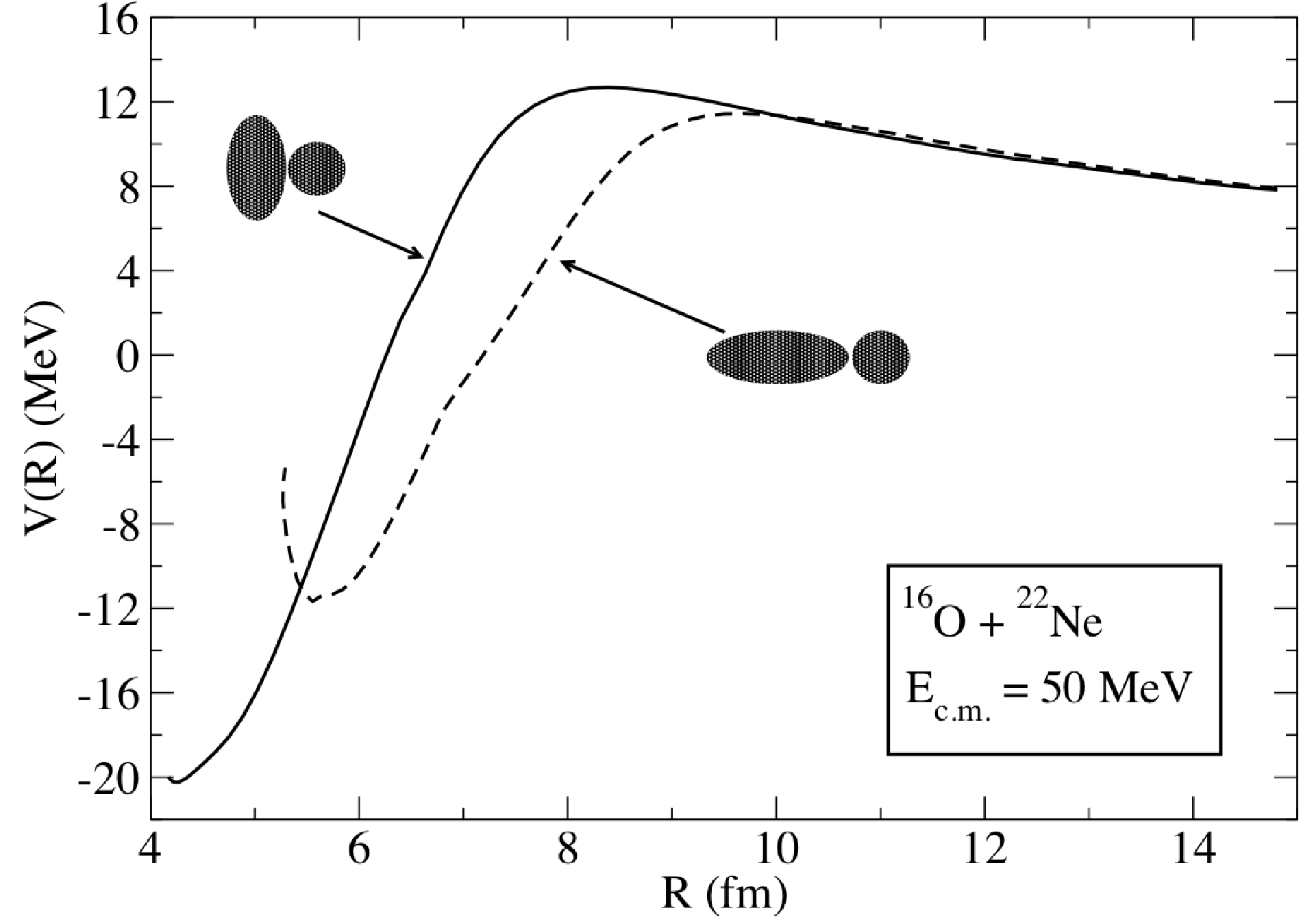
This effect is illustrated in figure 12 where potentials extracted from TDHF calculations are displayed as a function of relative distance for two different initial orientations of a prolate nucleus. In this case, when the orientation and collision axis are parallel, the contact between nuclei takes place at larger relative distance as compared to the perpendicular case which leads to a more compact configuration. The fusion barrier is then reduced for the parallel case because the Coulomb repulsion is smaller when the nuclear attraction starts to be significant. We also note in Fig. 11 that barriers distributions are peaked for compact configurations. This means that the probability that the system goes through a high energy barrier is higher than the one associated to low energy barriers. This is due to the fact that the deformed nucleus is prolate and not oblate. Let us consider for simplicity that the collision axis is the axis and that the deformation axis could only take three orientations along , or with equal probabilities. For a prolate nucleus (the elongation occurs along the deformation axis), the compact configuration (associated to higher barriers) is reached if the deformation axis is or , then with a probability . Having a lower barrier is then less probable, corresponding to a deformation along with a probability . The opposite occurs with an oblate nucleus (the elongation is perpendicular to the deformation axis). In this case, only an orientation along the axis leads to a compact configuration, then with a probability . This simplified discussion gives a qualitative understanding of figure 11.
In the simple discussion above, we have assumed that the distribution of relative orientations is isotropic. This hypothesis generally breaks down due to the long range Coulomb interaction which tends to polarize the nuclei during the approaching phase. In the case of a prolate nucleus, the Coulomb repulsion being stronger on the closest tip of the deformed nucleus, the net effect is to favor orientations where the deformation axis is perpendicular to the collision axis. This polarization effect modifies the simple isotropic picture, in particular when the deformed nucleus is light and its collision partner heavy [98].
In summary, we have seen that barrier position and height can be affected by the structure of the collision partners. It is hazardous to conclude that fusion could be a tool to infer nuclear structure properties. However, with precise fusion measurement, one can clearly get informations on deformation properties which might be hardly reached with other classical techniques of spectroscopy.
III.2.4 Excitation functions
The calculations presented in the previous section were performed using TDHF at zero impact parameter. To compute excitation functions (Fig. 3), calculations should include all impact parameters up to grazing. The fusion cross section is given by Eq. (57) where is nothing but the fusion probability for a given center of mass energy and angular momentum . The independent particle hypothesis implies that for and for . This finally leads to the so-called ”quantum sharp cut-off formula” [15]
| (62) |
To avoid discontinuities due to the cut-off and integer values of , is generally approximated by its semi-classical equivalent . The latter corresponds to the classical angular momentum threshold for fusion and denotes the maximum impact parameter below which fusion takes place [12]. This replacement is justified by the fact that and are both greater than and lower than . Accordingly, we finally obtain the standard classical expression for fusion cross sections .

Figure 13 presents a comparison between calculated and experimental cross sections for the 16O+208Pb system. Discretizing the impact parameters gives an upper and lower bound for fusion cross sections. We essentially see that above the fusion barrier, TDHF calculations reproduce rather well the experimental observations (the cross section is however slightly overestimated by 16%) while at energies below the Coulomb barrier, the calculation misses the quantum tunneling contribution.
III.3 Nucleon transfer around the fusion barrier
In this section, we study nucleon transfer below the fusion barrier with TDHF. The basic observable associated to transfer is simply the mass (or nucleon number) of the two fragments after re-separation. If the latter differs from the entrance channel, this is an obvious signature of transfer [118]. Another signature would be the variance of nucleon number in the fragments.
III.3.1 Transfer identification
As illustrated in figure 8, two nuclei can form a di-nuclear system with a neck and then re-separate. There is a priori no reason that these two fragments conserve the same neutron and proton numbers as in the entrance channel (except for symmetric reactions). Indeed, between the touching and re-separation, nucleons can be exchanged. In TDHF calculation, this exchange is treated through the time-dependent distortion of single-particle wave-function which can eventually be partially transfered from one partner to the other.
The following operator written in r-space defines the number of particles in the right side of the separation plane (defined arbitrarily as ):
| (63) |
where is the Heavyside function equal to 1 if and 0 elsewhere.
Denoting by the overlap (limited to the right side) between two single-particle states and using Eq. (196) for an independent particles state , we obtain (in the specific basis which diagonalizes the one-body density associated to )
| (64) |
Figure 14 gives the average final neutron and proton numbers of the smallest fragment in exit channels of 16O+208Pb reaction as a function of center of mass energy. We see that the more the energy increases, the more the 16O looses protons. At an energy just below the barrier, it has transfered around protons to the 208Pb. A possible explanation is the fast equilibration which is expected to take place at contact. Indeed, considering the case where exactly two protons have been transfered leads to the chemical equation
where quantities in parenthesis correspond to the values. We see that the initial asymmetry is almost equilibrated in the exit channel. This equilibration process also takes place at the first instant of fusion, and is increased when differences between partners increase [23, 36, 96, 99].
Note finally that these results on transfer agree qualitatively with what is observed experimentally [120]. Indeed, it is observed that the one proton transfer channel from 16O to 208Pb dominates below the Coulomb barrier, while at higher energies the two protons transfer becomes the main transfer channel.

III.3.2 Many-Body states associated to each fragment
Well below the fusion barrier, transfer is prohibited and exiting fragments essentially reflect mass and charge properties of the entrance channel. In this case, the 16O remains an eigenstate of the proton and neutron number operators99 9 We may introduce the terminology that a Many-Body state has a ”good” neutron (or proton) number when the state is an eigenstate of the particle number .. For these state, the variance of particle number operator (in the right side) is strictly zero: .
This property is lost at higher energies where transfer occurs. Then each fragment in the exit channel does not have a ”good” particle number and can therefore not be associated anymore to a single Slater determinant. It corresponds to a (eventually complicated) correlated state even if the wave-function associated to the total system is a Slater determinant.
Let us calculate the variance of after the reaction. We follow here the technique of Dasso et al. [39]. Using anti-commutation relations (141), closure relation , and Eq. (194), we get in the same way as for Eq. (64)
| (65) | |||||
| (66) |
The variance must then follow
| (67) |
Applying this formula to the small fragment in the exit channel at a center of mass energy 74.44 MeV, we get for protons and for neutrons. This deviation from zero clearly indicates that the Many-Body state on each side of the separation plane is not a pure state with a good particle number anymore but a complicated mixing of states with various particle numbers. In addition, even if the neutron number is almost constant in average, this non-zero variance is a signature of neutron transfer.
Note finally, that the variance is maximum when the overlap (restricted to the right side) between two wave-functions is zero, i.e. if . Then Eq. (67) identifies with a binomial distribution
| (68) |
This gives an upper limit for the variance
| (69) |
This upper limit is an intrinsic limitation of independent particle systems which will not be able to reproduce distribution with fluctuations greater than this limit. This is a clear limitation of TDHF, which in general underestimates widths of fragments mass and charge distribution observed in deep inelastic collisions [39, 48]. The account for correlation beyond the single-particle approximation is the only way to escape this difficulty.
III.4 Summary: success and limitations of TDHF
In this section, we have compared TDHF calculation with experiments on the different following physical effects and quantities
-
Barriers positions and height
-
Shape of barrier distribution for deformed nuclei
-
Excitation function
-
Populations of fragments mass and charge below the fusion barrier.
Overall, TDHF gives a reasonable qualitative (and sometimes quantitative) agreement with experiments. We have also pointed out some of the limitations of TDHF:
-
Essentially tunneling below the Coulomb barrier is not accounted for
-
Fluctuations of one-body observables like particle numbers are underestimated.
Beside nuclear reactions, differences between TDHF calculations and experiments could also be observed in giant collective vibrations. For instance, damping of collective motion could not be properly accounted for at the mean-field level [68]. This could again be traced back to missing two-body correlations effects. The rest of this lecture is devoted to transport theories going beyond mean-field.
IV Dynamical theories beyond mean-field
In the previous sections, we have illustrated some successes of mean-field theories in the description of nuclear dynamics. The application of TDHF to nuclear excitations or reactions was a major advance. At the same time, the mean-field theory neglects physical effects which play a major role in nuclei. For instance short and long range correlations in static nuclei could only be accounted for by a proper treatment of pairing effects and configuration mixing [13]. Conjointly, as the collision energy between two nuclei increases, the Pauli principle becomes less effective to block direct nucleon-nucleon collisions. Then, two-body correlations should be explicitly accounted for. The description of such two-body effects is crucial since, for instance, this would be the only way to understand how a nucleus could thermalize. During the past decades, several approaches have been developed to introduce correlations beyond mean-field. We summarize here some of these extensions.
IV.1 Time-dependent mean-field with pairing correlations
Pairing correlations are sometimes needed to describe nuclear systems.
However, they are neglected in the independent particles
approximation [93, 28]. Mean-field approaches could naturally incorporate
this effect by considering more general Many-Body states as products of
independent quasi-particles.
This leads to the so called Time-Dependent Hartree-Fock-Bogoliubov (TDHFB) theory.
IV.1.1 Quasi-particle vacuum
Wick’s theorem (see appendix A) simplifies the calculation of observables expectation values on vacuas. In appendix E, we show, on one hand, that an independent particles state is a vacuum (called HF vacuum) for a specific set of operators, and, on the other hand, is a simple example of ”quasi-particle” vacuum. The canonical and unitary transformation connecting quasi-particle creation and annihilation operators (denoted by and respectively) to particle ones is given by Eq. (E). It is called Bogolyubov transformation [19]. The vacuum associated to these quasi-particle operators is given by
| (70) |
which obviously insures . This state is then called a quasiparticle vacuum.
Let us illustrate how pairing could be included in such a Many-Body state. We consider the specific case where the transformation is simply written as
| (71) |
In this case, corresponds to the occupation probability of the state while . Eq. (71) is nothing but the standard BCS transformation [10] where single-particle states and form a Cooper pair. We use the standard convention . Starting from Eq.(70), grouping quasi-particles operators by pairs and using anti-commutation rules (140-141), we can rewrite the Many-Body state as
| (72) |
The above expression corresponds to the standard BCS state expressed in terms of pairs of correlated nucleons . In fact, any general Bogolyubov transformation can be written in a BCS form using the Bloch-Messiah-Zumino decomposition theorem [17, 126, 93]. We therefore see that to account for more general Many-Body states is a way to incorporate correlations beyond mean-field.
IV.1.2 Expectation values of observables on quasi-particle vacua
Similarly to HF vacua, the Wick’s theorem applies to Quasi-particle vacua. In this case, however, contractions associated to the one-body density are not the only one which differ from zero. The anomalous density, with matrix elements (which also implies ) should also be taken into account. The latter contractions cancel out for independent particle systems. The Bogolyubov transformation (Eq. (E)) can be inverted to express the and in terms of quasi-particles operators :
Using these expressions in et and the fact that only differ from zero, we deduce
| (76) |
These contractions are used to write the generalized density matrix defined as
The anomalous density enables us to treat correlations that were neglected at the independent particles level. Indeed, elements of the associated two-body correlation now read
| (83) | |||||
Countrary to Slater determinant, does not a priori cancels out. We further see that the HFB theory leads to a separable form of the two body correlation
| (84) |
In turns, HFB is more complex than the HF case. For instance, the state is not anymore an eigenstate of the particle number operator. The symmetry associated to particle number conservation is explicitly broken. Fluctuations associated to the particle number now write
| (85) |
In general these quantity is non-zero for a quasi-particle vacuum. The fact that the particle number is not conserved implies that it has to be constrained in average in nuclear structure studies (this is generally done by adding a specific Lagrange multiplier to the variational principle). It is worth mentioning that in a TDHFB evolution using a (possibly effective) two-body interaction (Eq. (5)), the expectation value of is a constant of motion. Therefore, no constraint on particle number is necessary in the dynamical case.
IV.1.3 TDHFB Equations
Different techniques could be used to derive the equation of motion in the HFB approximation [93, 13, 16]. Here, the same strategy as section II.2 is followed. The evolution of the Many-Body HFB state is given by the evolution of its normal and anomalous densities and which are given by the Ehrenfest theorem
| (86) | |||||
| (87) |
One-body density evolution
Eq. (86) can be identified to Eq. (34) which has been obtained for any correlated state and any two-body Hamiltonian. The only difference comes from the simplified correlations for quasi-particle vacua (Eq. (84))
| (88) | |||||
where we have introduced the pairing field
| (89) |
Evolution of
Similarly, the equation of motion for the anomalous density reads
| (90) | |||||
Eqs. (88) and (90) give the evolution of the matricies and
| (91) | |||||
| (92) |
Finally, using the generalized density matrix and the generalized HFB Hamiltonian defined as
Eqs. (91) and (92) can be written in a more compact form
| (96) |
The above TDHFB equation generalizes the TDHF case (Eq. (36)) by accounting for pairing effects on dynamics.
IV.1.4 Application of TDHFB theory
In practice, numerical implementation of TDHFB is much more complex than the TDHF case. This is certainly the reason why, although first applications of TDHF started more than 30 years ago, very few attempts to apply TDHFB exist so far. This could be traced back to conceptual and practical difficulties inherent to this theory. The first difficulty comes from the fact that TDHFB equations should a priori be solved in a complete single-particle basis while at the HF level only occupied states are necessary. In practice, specific methods should be used to truncate the basis. A second additional problem is the effective force that should be used in the pairing channel. Though zero range forces are clearly very useful at the HF level, they lead to ultra-violet divergences in the pairing channel. In practice, either a finite-range interaction has to be used or a specific regularization or renormalization scheme should be applied [44, 29, 30, 31]. Although these methods provide reasonable solutions for the static case, their application to nuclear dynamics is not straightforward.
IV.2 When is the independent particle approximation valid ?
In previous sections, we have considered dynamical evolutions where the many-body state is forced to remain in a specific class of trial state (Slater determinants or more general quasi-particle vacua). This assumption could only give an approximation of the exact dynamics and we do expect in general that the system will deviate from this simple state hypothesis. We give here some motivations of the introduction of theories beyond mean-field.
Let us recall the original goal which is to describe as best as possible the dynamics of a self-bound complex quantum system. We first assume that a system is initially properly described by a Slater determinant1010 10 The discussion below can easily be generalized to an initial quasi-particle vacuum, i.e. with where the label refers to initially occupied states (hole states). The exact dynamics of the system is given by the time-dependent Schroedinger equation (Eq. (2)). Unless the Hamiltonian contains one-body operators only, the mean-field theory can only approximate the exact evolution of the system.
IV.2.1 Decomposition of the Hamiltonian on particle-hole (p-h) basis
To precise the missing part, we complete the occupied states by a set (possibly infinite) of unoccupied single-particle states (also called particle states) labeled by (associated to the creation/annihilation and ). The completed basis verifies
| (97) |
From the above closure relation, any creation operator associated to a single-particle state decomposes as
| (98) |
The particle-hole basis is particularly suited to express any operator applied to the state due to the properties
| (99) |
For instance, restarting from the general expression of (Eq. (5)) the different single-particle states can be expressed in the particle-hole basis (Eq. (98)). Then, using anti-commutation relations (140) et (141), and as well as (20), (31), (35) et (99), we finally end with
where corresponds to the Hartree-Fock energy.
The above expression is helpful to understand the approximation made at the mean-field level. In previous section, we have shown that mean-field provides the best approximation for one-body degrees of freedom using the Ehrenfest theorem. In appendix G, we show that the mean-field evolution can be deduced using the Thouless theorem [105] and an effective Hamiltonian where is neglected.
IV.2.2 Limitation of the mean-field theory
In expression (IV.2.1), a clear separation is made between what is properly treated at the mean-field level ( and ) and what is neglected, i.e. . The latter is called ’residual interaction’. At this point several comments are in order:
-
The validity of the mean-field approximation depends on the intensity of the residual interaction which itself depends on the state and therefore will significantly depend on the physical situation. Starting from simple arguments [75], the time over which the Slater determinant picture breaks down could be expressed as:
(105) In the nuclear physics context, typical values of the residual interaction leads to fm/c. Therefore, even if the starting point is given by an independent particle wave-packet, the exact evolution will deviate rather quickly from the mean-field dynamics. This gives strong arguments in favor of theories beyond TDHF in nuclear physics.
-
An alternative expression of the residual interaction which is valid in any basis, is
(106) This expression illustrates that the residual interaction associated to a Slater determinants could be seen as a ”dressed” interaction which properly accounts for the Pauli principle. Physically, the residual interaction corresponds to direct nucleon-nucleon collisions between occupied states (2 holes) which could only scatter toward unoccupied states (2 particles) due to Pauli blocking. We say sometimes that the residual interaction has a 2 particles-2 holes (2p-2h) nature.
Due to the residual interaction, the exact many-body state will decompose in a more and more complex superposition of Slater determinants during the time evolution. As stressed in the introduction of this lecture, due to the complexity of the nuclear many-body problem, the exact dynamics is rarely accessible. In the following section, methods to include correlations beyond mean-field, like direct nucleon-nucleon collisions or pairing, are discussed.
IV.3 General correlated dynamics: the BBGKY hierarchy
Using the Ehrenfest theorem (section II.1.4), we have shown that the mean-field theory is particularly suited to describe one-body degrees of freedom. A natural extension of mean-field consists in following explicitly two-body degrees of freedom. Considering now the Ehrenfest theorem for the one and two-body degrees of freedom leads to two coupled equations for the one and two-body density matrix components and
| (107) |
Above equations are the two first equation of a hierarchy of equations, known as the Bogolyubov-Born-Green-Kirkwood-Yvon (BBGKY) hierarchy [18, 25, 62] where the three-body density evolution is also coupled to the four body density and so on and so forth. Here, we will restrict to the equations on and which have often served as the starting point to develop transport theories beyond mean-field [33, 89, 1, 68].
IV.4 The Time-Dependent Density-Matrix Theory
Previously, we have shown that the mean-field dynamics neglect two-body and higher correlations. Then the equations on reduce to TDHF. A natural extension which includes two-body effects is to treat explicitly two-body correlations and neglect only three-body () and higher correlations1111 11 Introducing the permutation operator between two particles, defined as . The two-body correlation matrix is given by: (108) while the three-body correlations reads (109) . The resulting theory where the one-body density and the two-body correlation are followed in time is generally called Time-Dependent Density-Matrix (TDDM) theory (see for instance [33])
| (110) |
where we have dissociated explicitly three terms which will be responsible for the build up of correlations in time. The Born term, , contains the physics of direct in-medium nucleon-nucleon collisions. Comparing and Eq. (106), we see that it is directly proportional to the residual interaction. Indeed, starting from a Slater determinant (), this is the only term that do not cancel out in the evolution of over a short time scale. In particular, it will be responsible for the departure from an independent particle picture. The physical interpretation of the term and is less straightforward. For instance, it has been shown that could be connected to pairing correlations [110] (see discussion below) while contains higher order and correlations. It is finally worth mentioning, that the last term could eventually be modified to better account for conservation laws (see discussion in [86]).
Application of the TDDM theory faces two major difficulties. First, since we are considering explicitly two-body degrees of freedom, we have to deal numerically with huge matrices and appropriate truncation schemes should be performed. Second, numerical applications are mainly possible with contact interaction (Skyrme like). These interactions, which are zero range in -space are thus of infinite range in momentum space. This unphysical behavior of the interaction is critical in practice, since during nucleon-nucleon collisions, particles may scatter towards too high momentum. No clear solution to this problem exists so far in the TDDM theory [68]. Due to these difficulties, only few applications have been carried out so far for collective vibrations [42, 76, 107, 108], and very recently for nuclear collisions [109].
IV.5 Link between TDDM and TDHFB
The connection between the TDDM and TDHFB has been clarified in Ref. [110]. Assuming a separable correlation in the p-p and h-h channels given by equation (84) gives
| (111) | |||||
where is nothing but the pairing field introduced above. Then, the one-body density evolution reduces to
| (112) |
In Ref. [110], it has been shown that neglecting and in the second equation of (110) leads to a TDHF like equation. Keeping only and assuming (84) leads to
| (113) | |||||
where we have identified the terms proportional to et . We then get
| (114) |
Using the expression of the pairing field (Eq. (89)), we finally recover the TDHFB equation (92). The above equation does not insure that the correlation matrix remains separable during the time-evolution. However, assuming that is valid for all time, the equations of motion identify with the TDHFB equation. It is worth mentioning that the above technique gives an alternative derivation of the TDHFB equation starting from TDDM which in addition illustrates the physical content of .
IV.6 Extended and Stochastic Time-Dependent Hartree-Fock
The pairing correlations become less important when the internal excitation of the system increases. In this case, direct nucleon-nucleon collisions are expected to dominate correlations beyond mean-field. A possible way to treat the latter and to escape part of the complexity of TDDM is to focus on the one-body density while the effect of correlations on this quantity is only treated approximatively. This could be done by neglecting the terms and in the evolution of [124, 125, 38, 26, 4]. Then, the equation for the two-body correlations takes a simple form
| (115) |
Solving this equation formally, we can develop the correlations over a time interval from an initial time to a time as
| (116) |
where represents the independent particle propagation of two particles with . In expression (116), the first term in the right hand side represents correlations developed by the residual interaction during the time interval. The second term describes propagation of the initial correlations from to , i.e. . Reporting this expression in the evolution of , we end up with a generalization of the TDHF theory (where we omit the label ”1” in )
| (117) |
where , called collision term, reads
| (118) |
while is given by
| (119) |
The term , which accounts for the initial correlation , dominates around . This term, in principle, contains all order correlations that are accumulated up to time , and it is a priori a very complicated quantity. Its treatment is clearly out of the scope of a one-body transport theory and statistical assumption is generally made on the initial correlations. It is assumed that the exact two-body correlations accumulated until exhibits random fluctuations. As a result, the average value of the initial correlations vanishes. This assumption is known as the ”molecular chaos assumption” in classical transport theory and it corresponds to factorization of two-particle phase-space density before each binary collision [58, 55]. Eq. (117) is then replaced by an ensemble of one-body evolutions
| (120) |
where now refers to the particular stochastic path and where is a fluctuating operator which vanishes in average. The complete statistical description of can be found in Refs. [6, 68]. Eq. (120) is the starting point of most of the microscopic transport theories that are applied nowadays in Heavy-Ion reactions at intermediate energies. However, due to its complexity, mainly the semi-classical version of Eq. (120), known as Boltzmann Langevin theory, has been applied to realistic situations (for a recent review, see [37]). Such a semi-classical approximation is not expected to apply in low energy nuclear reactions and we will concentrate here on its quantum version.
IV.6.1 Average evolution: irreversible process in Extended TDHF
We first concentrate on the average evolution and illustrate advantages of the introduction of a collision term on top of the mean-field dynamics. Averaging Eq. (117) over different trajectories leads to an equation where is replaced by the average one-body density, denoted by and where only the collision term remains. The resulting theory is called Extended TDHF with a non-Markovian collision term (or with ”memory effects”). The terminology ”non-Markovian” (in opposition to ”Markovian”) comes from the fact that the system at time depends not only on the density at time but also on its full history due to the presence of a time integral in Eq. (118).
At any time, eigenstates of , denoted by could be found. In this basis, called hereafter natural basis or canonical basis, reads
| (121) |
Using the weak coupling approximation in combination with the first order perturbation theory, the ETDHF equation can be transformed into a generalized master equation for occupation numbers which accounts for the Pauli principle
| (122) |
where the explicit form of the gain and loss kernels can be found in Ref. [65]. Therefore, in contrast to TDHF where occupation numbers are constant during the time evolution, in ETDHF the evolve and could eventually relax toward equilibrium. Such a relaxation is the only way to properly account for thermalization process in nuclei. The inclusion of correlation effect with Extended TDHF has been tested in the simplified case of two interacting nucleons in one dimension [65]. In this case, the exact dynamics could be solved numerically. In Fig. 15, starting from an initially uncorrelated state, the exact evolution of single-particle occupation numbers is compared to the Extended TDHF prediction.

Fig. 15, shows that the Extended TDHF is able to reproduce fairly well the evolution of one-body occupation numbers and one-body observables over long time. This result is very promising and indicates that Extended TDHF seems to be an appropriate theory for the description of dissipation when the residual interaction is weak. The above application has also demonstrated the importance of memory effects to properly describe quantum interacting systems although it significantly increases numerical efforts.
IV.6.2 Discussion on Stochastic mean-field dynamics
Due to the underlying hypothesis of Extended TDHF, such an average theory is expected to apply only over short time scale. The long time dynamics requires to include both dissipation and fluctuations and therefore to solve explicitly the stochastic version of the transport theory (Eq. (120)). Up to now, stochastic mean-field has been essentially applied in the semi-classical limit neglecting explicitly non-Markovian effects. Only recently, the theory proposed in Ref. [6] was used to study small amplitude collective vibrations in quantum system [66, 68] including full memory effects. In that case, the description of damping of giant resonances is greatly improved by including both dissipative and fluctuating kernels. However, due to numerical as well as conceptual difficulties, the application of the above stochastic quantum mechanics to large amplitude collective motion, like nuclear collisions, remains an open problem.
At this point, it is worth mentioning that extensive works have been devoted to the formal derivation of dissipative quantum mechanics [58] and/or related stochastic equations for fermions, including Markovian and non-Markovian effects [4, 9, 5, 6, 87, 88, 85]. These approaches have in common that the residual part of the interaction introduces disorder on top of the mean field. Such theories end with rather complex transport equations which are hardly applicable in realistic situations like Heavy-Ion collisions. Connections have been made recently between the dissipative equations of the one-body density and quantum jumps between Slater determinants using either perturbation theory or the connection between ETDHF [87, 88] and Lindblad equations [70] generally found in the theory of open quantum systems [27]. These theories, in which the many-body density are explicitly replaced by an average over Slater determinant densities, i.e. where each Slater determinant evolves according to a Stochastic TDHF equation, open new perspectives.
IV.7 Functional integrals and exact treatment of Many-Body correlated systems with Stochastic mean-field theories
IV.7.1 General Discussion
Starting from a simple Slater determinant state , correlations will develop in time and we do expect that the exact Many-Body state writes
| (123) |
where denotes a complete (eventually time-dependent) basis of Slater-Determinant states. Accordingly, the many-body density writes (see appendix C)
| (124) |
The extended and stochastic version of TDHF presented in sections IV.6, implicitly assume that the many-body density can be properly approximated by its diagonal components [87, 70]
| (125) |
where . Then a probability obeys master equations which eventually could be simulated by quantum jumps. The resulting density is obtained through the average over different stochastic paths, i.e.
| (126) |
Physically, this could be understood as follows. The irrelevant degrees of freedom (complex internal degrees of freedom) interact with the relevant degrees of freedom (single-particle degrees of freedom) and induce a fast decay towards zero of the off-diagonal matrix elements. This phenomenon is known as a decoherence process [64, 61]. It is clear, that such an approximation is associated with a loss of some quantum effects such as interferences between different channels. Therefore we do expect that most of the extensions of TDHF presented above, as TDHF, will miserably fail to account for most of the true Many-Body quantum effects.
The goal of the present section is to demonstrate that one could always treat exactly the Many-Body density given by Eq. (124) using an appropriate stochastic process between Slater determinants. Since there is no free lunch, the exact density is then obtained by an average
| (127) |
where states in the left differ from states on the right.
IV.7.2 Functional Integral technique in a model case
Functional integrals techniques have often been used to replace the exact Many-Body problem by an average over different ”effective” one-body problem [73, 74, 84]. In Ref. [63], the general strategy to obtain ground state properties of a many-body system using Monte-Carlo methods, the so called Shell-Model Monte-Carlo, is described. Recently, this technique has been combined with mean-field theory to obtain Stochastic TDHF equations which in average leads to the exact evolution [32, 57]. We give here a brief description of the method.
IV.7.3 Simple Introduction to functional integrals
We again consider that at a given time, the Many-Body state is a Slater Determinant . For a short time step , we have
| (128) |
Due to the presence of a two-body interaction in , the state differs from a Slater Determinant. Let us show how it can be written as a sum of Slater Determinants. For simplicity, we first assume that , where and are both one-body operators. Therefore corresponds to a two-body interaction. We introduce the notation for a normalized gaussian probability of the variable with mean zero and variance
| (129) |
We define the complex number and the one-body operator written as
| (130) |
Considering the average value of and keeping only terms up to , we obtain
| (131) |
By averaging over the different realizations of , we recover the exact propagator over a short time step. Note that more general relations could be found using the Hubbard-Stratonovish transformation (see for instance [63]). Using the above relation, we see that
| (132) |
Due to the one-body nature of , each is a Slater determinant. Indeed, according to the Thouless theorem [105] (see appendix G, an exponential of a one body operator transforms a Slater determinant into another Slater determinant. We have therefore demonstrated that the evolution of the exact state could be replaced by an ensemble of Slater determinants. The method could then be iterated for each to obtain the long-time evolution as a superposition of independent particle states.
Several comments are in order:
-
Starting from a Many-Body density written as , at an intermediate time, the average density writes
(133) with two states, where evolves according to Eq. (134) while evolves according to
(134) where is a noise independent of , with mean zero and . Since the evolution is exact, any one-, two- or k-body observable estimated through will follow the exact dynamics.
IV.7.4 General two-body Hamiltonian
In previous section, we have illustrated how the exact dynamics of a system could be replaced by a set of stochastic evolutions of several Slater determinants using a schematic two-body Hamiltonian. We now start from the general expression of the Hamiltonian (IV.2.1) to introduce the exact Stochastic Mean-field (SMF) technique. In this expression, the Hamiltonian is naturally splitted into a mean-field part and a two-body residual interaction . It turns out that this interaction can always be decomposed as a sum of square of one-body operators [63]
| (135) |
where is a one-body operator while denotes a set of constants (eventually complex). The discussion in the previous section can then easily be generalized. The residual interaction factorizes as
| (136) |
where . Therefore, for realistic interactions one should introduce as many stochastic Gaussian independent variables as the number of operators entering in the sum. In practice, this number defines the numerical effort which in general is very large. For this reason, only few applications to the dynamics of rather simple systems exist so far. Finally, the extension of above stochastic theories to HFB states can be found in Ref. [71] while an explicit link with observables evolutions is studied in Refs. [72, 69].
IV.8 Summary
In this section, we have summarized some of the possible ways to extend TDHF, some of them are able to incorporate pairing correlations (like TDHFB or TDDM) while others concentrate on direct nucleon-nucleon collisions (ETDHF). Though promising, these theories to the nuclear many-body problem remain very challenging to apply.
A second difficulty which has been largely hidden in the present lecture is that all applications of dynamical quantum transport theories, like TDHF, to nuclear reactions was possible only because of the introduction of effective interactions (essentially Skyrme like). These interactions have led to the more general concept of Energy Density Functional (EDF) and are expected, in a similar way as the Density Functional Theory (DFT) in condensed matter, to incorporate most of the correlations already at the mean-field level. Then, the notion of ”beyond mean-field” calculations becomes ill defined. For instance, all theories (extended, stochastic, functional…) start from a Many-Body Hamiltonian. In the EDF context, such an Hamiltonian, although it exists, is not simply connected to the EDF itself. As a consequence, the Hamiltonian derivation could serve as a guideline but a proper formulation in the EDF framework is mandatory. Large debates exist nowadays on the validity and foundation of the nuclear EDF applied to static properties of nuclei. Similar discussion should be made on what we should definitively call Time-Dependent EDF (TDEDF) and not ”TDHF”.
Acknowledgments
These lecture notes are dedicated to the memory of Paul Bonche, one of the most famous pioneer in the application of TDHF to nuclear physics and author of the 3D TDHF code that has been used in most of the applications presented here.
We also thank our collaborators working in nuclear structure and using similar techniques based on mean-field theory for various discussions. Last, we thank Andrea Vitturi for his contribution on the fusion part.
Appendix A Basics of quantum mechanics
Here, we summarize some aspects of quantum mechanics and more specifically second quantization. Only concepts useful for the the present lecture notes are introduced (see [78, 16] for more details).
A.1 Single-particle creation/annihilation operators
The single-particle wave-function , with spin and isospin components denoted respively by and can be written as
| (137) |
The associated creation operator acting on the vacuum verifies
| (138) |
Its Hermitian conjugated is the annihilation operator For all annihilation operator, we have
| (139) |
This property defines the particle vacuum associated to the set of operators and .
We consider here fermions. The Pauli principle imposes that two identical fermions could not be created in the same state . Creation/annihilation operators verifies anti-commutation rules
| (140) | |||||
| (141) |
where .
It could be useful to go from one single-particle basis to another, and to express creation/annihilation of the first basis in terms of creation/annihilation of the second basis . To do so, the two basis should obviously represent the same Hilbert space (and be complete with respect to this space). Fort instance, the relation of any single-particle basis to the coordinate representation is
| (142) | |||||
| (143) |
Using the closure relation , previous relations can be inverted as
| (144) | |||||
| (145) |
A.2 identical particles state
We denote by a -body state which is a priori correlated. Occupation numbers of a correlated state, in opposite to an uncorrelated state, have values which might differ from zero and one. A independent particles state corresponds to a specific case where occupation numbers are exactly one while the other are zero. We not such a state . It can be written as an antisymmetric product of single-particle states (called Slater determinant due to its specific form, see Eq. (163))
| (146) |
where means that the particle 1 is in the state , particle 2 occupies state ,.. The coefficient insures the proper normalization of the wave while the anti-symmetrization operator writes
| (147) |
Here (resp. -1) for odd (resp. even) permutations of particles. For instance, its action on a two-particle wave-function reads
| (148) |
In second quantization, an independent particle state reads
| (149) |
A.3 Wick’s Theorem
The Wick’s theorem enables to simply express expectation values of observables for specific states (that could be considered as vacua). Let us first define the term contraction. Consider two creation and/or annihilation operators, denoted by and (these operators could also be linear combinations of creation/annihilation operators) and the associated vacuum. In practice, this vacuum could be a single-particle vacuum, a HF state denoted by or a quasi-particle (HFB) vacuum (see section IV.1). The contraction is defined as the expectation value of on the vacuum
| (150) |
Then, the Wick’s theorem states:
The expectation value of a product of creation/annihilation operators on their vacuum is equal to the sum of all possible products of contractions of pairs of operators, each product of contractions being multiplied by + or - depending on the parity of the permutation needed to put together the contracted operators.
Let us illustrate this on the overlap between two anti-symmetric two independent particles states
| (151) |
Contractions are given by and We then deduce
| (152) |
This result can be generalized to the overlap between two -particles Slater determinants constructed from two different basis and
| (153) |
We can then use the Wick’s theorem to express this overlap in terms of a determinant made of overlaps between single-particle states
| (154) |
A.4 Basis of particles states
Starting from a single-particle complete basis, we can always construct a basis of -body Slater determinants. For instance, we calculate the overlap between two Slaters formed from a priori different single-particle states of the same basis. According to Eq. (154), we have
This overlap is if and contain exactly the same occupied states and if at least one of the single-particle states is different. Therefore, two different Slater determinants are orthogonal. It could be shown finally that the set of Slaters constructed by picking up all possible combination of single-particle states forms a complete basis of the -body Hilbert space. In other words, any many-body state, correlated or not, can be written in the form
| (159) |
A.5 Independent particles wave-functions
The Wick’s theorem is also helpful to express the wave function of a particles state. We want to write a wave function in position-spin-isospin representation. Associated single-particle states are , where is the position, and the spin and isospin projections respectively. Using Eq. (146), a Slater built using this basis reads
| (160) |
The particles wave function is then given by
| (161) |
For an independent particle system, the wave function reduces to
| (162) |
From Eq. (154), we see that we simply obtain the standard Slater determinant formula
| (163) |
Let us check that this wave-function is properly normalized. Introducing the notation , the nomalization reads
| (164) | |||||
Developing the determinants and using , we finally get
| (172) | |||||
Finally, it is worth to mention, that, using Eq. (161) and (164), the closure relation for the particles states reads
| (173) |
Appendix B One-body observables
One-body observables are generally written as a sum of operators acting on each single-particle components independently,
| (174) |
In second quantization, one-body operators reads
| (175) | |||||
Both expressions lead to the same action on a -body wave function. For instance, considering the independent particle case, using Eqs. (174), (146), (148) and the notation , we have
| (176) | |||||
Eq. (175) leads to
| (177) |
Only occupied contribute due to Eq. 139 and we get
| (178) | |||||
where we have also used Eqs. (140) and (141). This result is nothing but Eq. (176). The table 2 gives few examples of one-body operators commonly used in the nuclear reaction context.
| Observable | Standard form | Second quantization |
|---|---|---|
| Center of mass position | ||
| Center of mass momentum | ||
| Particle number | ||
| Monopole operator | ||
| Quadrupole operator |
Appendix C Density matrices
The -body density matrix of a particle system (described by ) contains all the information on the system. It could be written as an operator acting on the -body Hilbert space as (see for example [104, 1, 68]). If we are only interested in the -body observables (), we do not need all the information carried by . A natural way to reduce the information is to introduce the -body density matrix of the state . It could be defined from as
| (179) |
Equivalently, the -body density matrix components are defined by the relation
| (180) |
In coordinate space (), it writes
| (181) |
Other notations, like , are also sometimes used. The main advantage of the -body density is that it contains all the information on the system as far as -body or lower observables are concerned. For instance, the expectation value of a -body observable reads
| (182) | |||||
Appendix D Two-body correlations
When we want to get the expectation value of a two-body observable, as it is the case for the Hamiltonian , we do a priori need the two-body density matrix of the system (see appendix C). The two-body density matrix can always be decomposed into an uncorrelated part (anti-symmetric product of one-body densities) and a correlation part, denoted by
| (183) |
The correlation operator can be seen as the part of the two-body density which cannot be written as a product of single-particle operators. It is also possible to use the notation
| (184) |
where corresponds to the permutation operator between particles 1 and 2. We recall that notations are equivalent. Note that higher -body correlations matrices (with ) could be defined in a similar way [68].
Appendix E Hartree-Fock and quasi-particle vacua
A Slater determinant is sometimes called HF vacuum. The state is indeed a vacuum for the creation operators and annihilation operators written, in the basis that has served to construct the many-body state, as
| (185) | |||||
| (186) |
where for occupied states (also called hole states) and 0 for unoccupied states (particle states). It could easily be checked that these new operators verify Eqs. (140) and (141) and that is a vacuum for them,
| (187) |
Slater determinants are a specific case of quasi-particle vacua. More generally, quasi-particle creation/annihilation operators are defined through a linear combination of single-particle creation/annihilation operators
where matrices et are chosen in such a way that the quasiparticle operators verify the fermionic anti-commutation rules (Eqs. (140-141)). The vacua associated to these operators can be written as
| (191) |
where is a normalization constant. We see that the latter expression insures .
Appendix F Two-body density for independent particle systems
We show here, using the Wick’s theorem, that it is equivalent to have the property and to consider a system of independent particles. Starting from a Slater determinant , using the fact that this state is a vacuum for the (see appendix E), and the inverse of Eqs. (185-186) in a given basis denoted by
| (192) | |||||
| (193) |
with or , we can use Wick’s theorem to express two-body matrix elements :
| (194) |
Here contractions are made with the HF state . Using and , we finally obtain that the two-body matrix elements read
| (195) |
Here, the two-body correlation is strictly zero. In the notes, we often used contractions in the specific basis of occupied states, which simply read
| (196) |
Appendix G Mean-field dynamics from the Thouless Theorem
Starting from Eq. (IV.2.1) and an initial Slater determinant, we neglect the residual interaction, i.e. we only keep in the dynamical evolution. Then, over an infinitesimal time step , the new state is approximated by
| (197) |
where , and . We recall that denotes an occupied state and an unoccupied one. As we will discuss below, to recover the single-particle evolutions, it is convenient to rewrite the Mean-Field Hamiltonian in a slightly different manner (using )
| (198) | |||||
where ”i” denotes a complete single-particle basis. The term does not influence the single particle evolution (we omit its contribution in the following). The propagator expressed as an exponential of one-body operators and therefore, according to the Thouless Theorem [105], transforms a Slater Determinant into another Slater determinant. Indeed, the fact that and allow us to write
Considering the transformation of each creation operator separately, we have
| (199) | |||||
where the expression of the mean-field operator defined in Eq. (IV.2.1) has been used. From the above identity, we see that the propagated many-body state writes where, using , the single-particle states evolve according to
| (200) |
which is nothing but the standard mean-field evolution. Therefore, we have shown in this appendix that the mean-field evolution is recovered by neglecting the two-body residual interaction.
The fact that we exactly recover the standard single-particle wave-function evolution is due to the specific way we have written the Mean-Field Hamiltonian in Eq. (198). If, instead, we take the original expression and use the fact that induces only a phase, then, using the same technique, we would get
| (201) |
These single-particle equation differs from the standard Eq. (200) but contains the same information. Indeed, we have
| (202) |
where we have recovered the correct one-body density evolution.
References
- [1] Y. Abe, S. Ayik, P.-G. Reinhard and E. Suraud, Phys. Rep. 275, 49 (1996).
- [2] V.I. Abrosimov, D.M. Brink, A. Dellafiore and F. Matera, 11th Int. Conf. on Nuclear Reaction Mechanisms, Varenna (Italy); nucl-th/0610087 (2006).
- [3] D. Almehed and P.D. Stevenson, J. Phys. G 31, S1819 (2005).
- [4] S. Ayik, Z. Phys. A 298, 83 (1980).
- [5] S. Ayik and C. Gregoire, Phys. Lett. B 212, 269 (1988).
- [6] S. Ayik and Y. Abe, Phys. Rev. C 64, 024609 (2001).
- [7] S. Ayik, D. Lacroix and Ph. Chomaz, Prog. Part. Nucl. Phys. 52, 497 (2004).
- [8] A.B. Balantekin and N. Takigawa, Rev. Mod. Phys. 70, 78 (1998).
- [9] R. Balian and M. Veneroni, Ann. Phys. 135, 270 (1981).
- [10] J. Bardeen, L.N. Cooper and J.R. Schrieffer, Phys. Rev. 108, 1175 (1957).
- [11] R. Bass, Phys. Rev. Lett. 39, 265 (1977) .
- [12] R. Bass, Nuclear Reactions (Springer-Verlag, Berlin, 1980).
- [13] M. Bender, P.-H. Heenen and P.-G. Reinhard, Rev. Mod. Phys. 75, 121 (2003).
- [14] M. Bender, Eur. Phys. J. Special Topics 156, 217 (2008).
- [15] J. S. Blair, Phys. Rev. 95, 1218 (1954).
- [16] J. Blaizot and G. Ripka, Quantum Theory Of Finite Systems (MIT Press, Cambridge, 1986).
- [17] C. Bloch and A. Messiah, Nucl. Phys. 39, 95 (1962).
- [18] N.N. Bogoliubov, J. Phys. (URSS) 10, 256 (1946).
- [19] N.N. Bogoliubov, Sov. Phys. JETP 7, 41 (1958).
- [20] A. Bohr and B. Mottelson, Nuclear Structure Vol. I, chapter 2 (Benjamin, Reading, MA., 1969).
- [21] P. Bonche, S. Koonin and J. W. Negele, Phys. Rev. C 13, 1226 (1976).
- [22] P. Bonche, B. Grammaticos and S. Koonin, Phys. Rev. C 17, 1700 (1978).
- [23] P. Bonche and N. Ngô, Phys. Lett. B 105, 17 (1981).
- [24] P. Bonche, H. Flocard and P.H. Heenen, Comp. Phys. Com. 171, 49 (2005).
- [25] H. Born and H.S. Green, Proc. Royl. Soc. A188, 10 (1946).
- [26] W. Botermans and R. Malfliet, Phys. Rep. 198, 115 (1990).
- [27] H.P. Breuer and F. Petruccione, The Theory of Open Quantum Systems (Oxford Univ. Press, 2002).
- [28] D.M. Brink and R.A. Broglia, Nuclear Superfluidity : Pairing in finite systems (Cambridge Univ. Press, 2005).
- [29] A. Bulgac and Y. Yu, Phys. Rev. Lett. 88, 042504 (2002).
- [30] A. Bulgac, Phys. Rev. C 65, 051305 (2002).
- [31] A. Bulgac and Y. Yu, Phys. Rev. Lett. 90, 222501 (2003).
- [32] I. Carusotto, Y. Castin and J. Dalibard, Phys. Rev. A 63, 023606 (2001).
- [33] W. Cassing and U. Mosel, Prog. Part. Nucl. Phys. 25, 235 (1990).
- [34] E. Chabanat, P. Bonche, P. Haensel, J. Meyer et R. Schaeffer, Nucl. Phys. A 627, 710 (1997).
- [35] E. Chabanat, P. Bonche, P. Haensel, J. Meyer et R. Schaeffer, Nucl. Phys. A 635, 231 (1998).
- [36] Ph. Chomaz, M. Di Toro and A. Smerzi, Nucl. Phys. A 563, 509 (1993).
- [37] Ph. Chomaz, M. Colonna and J. Randrup, Phys. Rep. 389, 263 (2004).
- [38] P. Danielewicz, Ann. Phys. 152, 305 (1984).
- [39] C.H. Dasso et al., Z. Phys. A 289, 395 (1979).
- [40] M. Dasgupta, D.J. Hinde, N. Rowley et A.M. Stefanini, Annu. Rev. Nucl. Part. Sci. 48, 401 (1998).
- [41] K.T.R. Davies, H. Flocard, S. Krieger and M.S. Weiss, Nucl. Phys. A 342, 111 (1980).
- [42] F.V. De Blasio et al., Phys. Rev. Lett. 68, 1663 (1992).
- [43] P.A.M. Dirac, Proc. Cambridge Philos. Soc. 26, 376 (1930).
- [44] J. Dobaczewski, H. Flocard and J. Treiner, Nucl. Phys. A 422, 103 (1984).
- [45] J. Dobaczewski, M.V. Stoistov, W. Nazarewicz and P.-G. Reinhard, Phys. Rev. C 76, 054315 (2007).
- [46] H. Flocard, S.E. Koonin and M.S. Weiss, Phys. Rev. C 17, 1682 (1978).
- [47] V. Fock, Z. Phys. A 61, 126 (1930).
- [48] Time-Dependent Hartree-Fock and Beyond, ed. K. Goeke and P.-G. Reinhard, Lecture Notes in Physics, vol. 171 (1982).
- [49] D. Gogny, Nuclear Self-Consistent Fields, ed. G. Ripka and M. Porneuf (North-Holland, Amsterdam, 1975) p. 333.
- [50] Lu Guo, J.A. Maruhn and P.-G. Reinhard, Phys. Rev. C 76, 014601 (2007).
- [51] Lu Guo, J.A. Maruhn and Y. Hashimoto, Phys. Rev. C 77, 041301 (R) (2008).
- [52] K. Hagino, N. Rowley and A.T. Kruppa, Comp. Phys. Comm. 123, 143 (1999).
- [53] D. R. Hartree, Proc. Cambridge Philos. Soc. 24, 89 (1928).
- [54] Y. Hashimoto and K. Nodeki, nucl-th/0707.3083 (2007).
- [55] K. Huang, Statistical Mechanics, (Wiley, N.Y., 1962).
- [56] F. Iachello and P. van Isacker, The Interacting Boson-Fermion Model (Cambridge Univ. Press, 1991).
- [57] O. Juillet and Ph. Chomaz, Phys. Rev. Lett. 88, 142503 (2002).
- [58] L.P. Kadanoff and G. Baym, Quantum Statistical Mechanics (Benjamin, N.Y., 1962).
- [59] E. Khan, N. Sandulescu, M. Grasso and Nguyen Van Giai, Phys. Rev. C 66, 024309 (2002).
- [60] K.-H. Kim, T. Otsuka and P. Bonche, J. Phys. G 23, 1267 (1997).
- [61] C. Kiefer et al., Decoherence and the Appearance of a Classical World in Quantum Theory (Springer, N.Y., 2003).
- [62] J.G. Kirwood, J. Chem. Phys. 14, 180 (1946).
- [63] S.E. Koonin, Ann. Rev. Nucl. Part. Sci. 47, 463 (1997).
- [64] O. Kuebler and H.D. Zeh, Ann. Phys. 76, 405 (1973).
- [65] D. Lacroix, Ph. Chomaz and S. Ayik, Nucl. Phys. A 651, 369 (1999).
- [66] D. Lacroix, S. Ayik and Ph. Chomaz, Phys. Rev. C 63, 064305 (2001).
- [67] D. Lacroix, cours de l’école Joliot-Curie (2002).
- [68] D. Lacroix, S. Ayik and Ph. Chomaz, Prog. Part. Nucl. Phys. 52, 497 (2004).
- [69] D. Lacroix, Phys. Rev. C 71, 064322 (2005).
- [70] D. Lacroix, Phys. Rev. C 73, 044311 (2006).
- [71] D. Lacroix, nucl-th/0605033 (2006).
- [72] D. Lacroix, Annals Phys. 322, 2055 (2007).
- [73] S. Levit, Phys. Rev. C 21, 1594 (1980).
- [74] S. Levit, J.W. Negele and Z. Paltiel, Phys. Rev. C 21, 1603 (1980).
- [75] P.C. Lichtner and J.J. Griffin, Phys. Rev. Lett. 37, 1521 (1976).
- [76] H.-G. Luo et al., Nucl. Phys. A 652, 164 (1999).
- [77] J.A. Maruhn, P.-G. Reinhard, P.D. Stevenson and M.R. Strayer, Phys. Rev. C 74, 027601 (2006).
- [78] A. Messiah, Mécanique Quantique (Dunod, 1959).
- [79] J. Meyer, cours de l’école Joliot Curie (2000).
- [80] S. Mitsouka et al., Phys. Rev. Lett. 99, 182701 (2007).
- [81] C.R. Morton et al., Phys. Rev. C 60, 044608 (1999).
- [82] T. Nakatsukasa and K. Yabana, Phys. Rev. C 71, 024301 (2005).
- [83] J.W. Negele, Rev. Mod. Phys. 54, 913 (1982).
- [84] J.W. Negele and H. Orland, Quantum Many Particles (Frontiers in Physics, Addison-Weysley pub. comp., N.Y., 1988).
- [85] A. Ohnishi and J. Randrup, Phys. Rev. Lett. 75, 596 (1995).
- [86] A. Peter et al., Nucl. Phys. A 573, 93 (1994).
- [87] P.-G. Reinhard and E. Suraud, Ann. Phys. 216, 98 (1992).
- [88] P.-G. Reinhard and E. Suraud, Nucl. Phys. A 545, 59 (1992).
- [89] P.-G. Reinhard and C. Toepffer, Int. J. Mod. Phys. E 3, 435 (1994).
- [90] P.-G. Reinhard, Y. Abe, S. Ayik and E. Suraud, Phys. Rep. 275, 49 (1996).
- [91] P.-G. Reinhard, Lu Guo and J.A. Maruhn, Eur. Phys. J. A 32, 19 (2007).
- [92] P.-G. Reinhard, P.D. Stevenson, D. Almehed, J.A. Maruhn and M.R. Strayer, Phys. Rev. E 73, 036709 (2006).
- [93] P. Ring and P. Schuck, The Nuclear Many-Body Problem (Springer-Verlag 1980).
- [94] N. Rowley, G.R. Satchler and P.H. Stelson, Phys. Lett. B 254, 25 (1991).
- [95] R.N. Sagaidak et al., in Proc. of VI International School-Seminar ”Heavy Ion Physics”, Dubna, 1997, ed. Yu. Ts. Oganessian and R. Kalpakchieva (World Scientific, Singapore, 1998), p. 323.
- [96] C. Simenel, Ph. Chomaz and G. de France, Phys. Rev. Lett. 86, 2971 (2001).
- [97] C. Simenel and Ph. Chomaz, Phys. Rev. C 68, 024302 (2003).
- [98] C. Simenel, Ph. Chomaz and G. de France, Phys. Rev. Lett. 93, 102701 (2004).
- [99] C. Simenel, Ph. Chomaz and G. de France, Phys. Rev. C 76, 024609 (2007).
- [100] C. Simenel and B. Avez, Int. J. Mod. Phys. E 17, 31 (2008).
- [101] K. Siwek-Wilczyńska, I. Skwira and J. Wilczyński, Phys. Rev. C 72, 034605 (2005).
- [102] T. Skyrme, Phil. Mag. 1, 1043 (1956).
- [103] J.R. Stone and P.-G. Reinhard, Prog. in Part. and Nucl. Phys. 58, 587 (2007).
- [104] E. Suraud, cours de l’école Joliot-Curie (1995).
- [105] D.J. Thouless, Nucl. Phys. 21, 225 (1961).
- [106] D.J. Thouless and J.G. Valatin, Nucl. Phys. 31, 211 (1962).
- [107] M. Tohyama and A.S. Umar, Phys. Lett. B 516, 415 (2001).
- [108] M. Tohyama and A.S. Umar, Phys. Lett. B 549, 72 (2002).
- [109] M. Tohyama and A.S. Umar, Phys. Rev. C 65, 037601 (2002).
- [110] M. Tohyama and S. Takahara, Prog. Theor. Phys. 112, 499 (2004).
- [111] M. Di Toro and V.M. Kolomietz, Z. Phys. A 328, 285 (1987).
- [112] A.S. Umar and V.E. Oberacker, Phys. Rev. C 71, 034314 (2005).
- [113] A.S. Umar and V.E. Oberacker, Phys. Rev. C 73, 054607 (2006).
- [114] A.S. Umar and V.E. Oberacker, Phys. Rev. C 74, 021601 (2006).
- [115] A.S. Umar and V.E. Oberacker, Phys. Rev. C 74, 024606 (2006).
- [116] A.S. Umar and V.E. Oberacker, Phys. Rev. C 74, 061601 (R) (2006).
- [117] A.S. Umar and V.E. Oberacker, Phys. Rev. C 76, 014604 (2007).
- [118] A.S. Umar, V.E. Oberacker and J.A. Marhun, nucl-th/0805.4156.
- [119] D. Vautherin and D.M. Brink, Phys. Rev. C 5, 626 (1972).
- [120] E. Vulgaris et al., Phys. Rev. C 33, 2017 (1986).
- [121] K. Washiyama and D. Lacroix, nucl-th/0804.2823 (2008).
- [122] H.A. Weidenmuller et al. , Ann. Phys. 139, 190 (1981).
- [123] C.Y. Wong, Phys. Rev. Lett. 31, 766 (1973).
- [124] C.Y. Wong and H.H.K. Tang, Phys. Rev. Lett. 40, 1070 (1978).
- [125] C.Y. Wong and H.H.K. Tang, Phys. Rev. C 20, 1419 (1979).
- [126] B. Zumino, J. Math. Phys. 3, 1055 (1962).