TU-819 RIKEN-TH-133
Extended MQCD and SUSY/non-SUSY duality
Kazutoshi Ohtaa** * E-mail:kohta@phys.tohoku.ac.jp and Ta-Sheng Taib†† † E-mail:tasheng@riken.jp
a Department of Physics, Tohoku University, Sendai 980-8578, JAPAN
b Theoretical Physics Laboratory, RIKEN, Wako, Saitama 351-0198, JAPAN
We study the SUSY/non-SUSY duality proposed by Aganagic et al. from Type IIA string and M-theory perspectives. We find that our brane configuration generalizes the so-called Seiberg-Witten theory on the one hand, and provides a way to realize non-SUSY vacua by intersecting NS5-branes on the other hand. We also argue how the partial SUSY breaking from down to can be clearly visualized through the brane picture.
1 Introduction
Recently, Aganagic et al. proposed a SUSY/non-SUSY duality [1] in Type IIB string compactification. In contrast to previous works [2, 3, 4] where anti-branes are introduced by hand, the breakthrough is to turn on a holomorphic varying background NS-flux through the non-compact Calabi-Yau (CY) three-fold. This soon suggests a way to realize various kinds of SUSY or non-SUSY vacua via adjusting parameters the NS-flux contains 11 1 Applications and generalizations of these flux vacua are also discussed in a recent paper [5]..
Let us briefly review their ideas. Because of the flux , four-dimensional gauge theory, realized by wrapping D5-branes on vanishing two-cycles of a CY, acquires different gauge couplings at each locus:
| (1.1) |
where parameterizes a CY bearing, say, the -type singularity as
| (1.2) |
Note that , providing a non-trivial fibration over , corresponds to the tree-level superpotential breaking down to . Also, the adjoint chiral field on D5-branes gets identified with the transverse -direction. Although generalizing to other ALE fibrations can be carried out, the above prototype will prove to be sufficiently good due to arbitrarily many degrees of freedom inside .
The proposed SUSY/non-SUSY duality is achieved by tuning coefficients of the -dependent background -field, which has the following expression22 2 As noted in [1], the degree of polynomial is restricted to at most for triviality of the operator in gauge theory chiral ring.
| (1.3) |
where denotes the ultraviolet prepotential33 3 In gauge theory, the bare coupling constant is determined by a holomorphic function as . . For generic , SUSY is spontaneously broken at UV. This is accounted for by (1.1), in which one observes that ’s may develop relatively different orientations at critical points for Kähler moduli of . On the other hand, some specific choice of can still make four supercharges preserved, i.e. all orientations of ’s are kept aligned. As shown in [1], through geometric transition to dual CY manifolds, SUSY breaking effects can as well be captured qualitatively by studying strongly-coupled IR physics. Minimizing the effective superpotential there, one can further determine from 44 4 This fact can be interpreted from the M-theory perspective, see below. .
Like the brane realization [6, 7, 8] of meta-stable SUSY breaking vacua [9], our purpose in this paper is to translate things considered above into Type IIA/M-theory language. It is well-known that via a T-duality acting on one instead obtains two NS5-branes in flat spacetime with D4-branes in between them. From the tree-level F-term
| (1.4) |
one can choose a vacuum such that the gauge group is broken to . Then, it is seen that D4-branes, coming from fractional D3-branes, remain at ’s. The size and orientation of controlled by (1.3) are translated, respectively, to the length along the T-dual direction (bare gauge coupling) and sign of RR charge of -th stack of D4-branes. Based on this Type IIA tree-level description55 5 As usual, we notice that tree-level field theory results match with classical brane pictures at the lowest order in under , i.e. brane bending and string interaction are not taken into account., which naively means negative gauge couplings can be understood as two crossing NS5-branes that result in anti-branes. How spontaneously SUSY breaking vacua occur can therefore be visualized clearly in the presence of both D4- and -branes as a consequence of the prepotential.
The rest of this paper is organized as follows. In the next section, we review some known facts about Type IIA/M-theory brane configurations. In section 3, we study the SUSY/non-SUSY duality by introducing a varying -field. We also comment on the partial SUSY breaking mechanism in terms of Type IIA brane pictures. Finally, we conclude in Section 4.
2 Type IIA/M-theory brane picture
To set up notations in this paper, we briefly review Type IIA/M-theory brane configurations here66 6 For more details, see [10] and references therein..
2.1 Type IIA setup
Viewing alternatively in (1.2) as an fiber over -plane, one can go from Type IIB CY geometry to Type IIA Hanany-Witten [11] type brane setup upon a T-daulity along this (-direction) [12, 13, 14, 15], namely,
| (2.1) |
Note that from now on our convention will be
| (2.2) |
To be precise, take a conifold
| (2.3) |
for example. By replacing the conifold tip with a , its singularity can be treated as if there is a two-center Taub-NUT space. Upon the well-known Taub-NUT/NS5 duality, T-dualizing along the Kaluza-Klein circle makes the geometry change to two perpendicular NS5-branes shown in Table 1. In addition, a complex separation arises due to the size of . The vanishing two-cycle assumption enables us to set .
| 0123 | 4 | 5 | 6 | 7 | 8 | 9 | |
| NS5 | |||||||
| NS5’ | |||||||
| D4 |
As far as concerned, near each critical point where , the geometry locally looks like a conifold. With a resolution on each singularity, after T-duality, two NS5-branes having common directions are represented as on -plane and separated along by . Furthermore, since D5-branes wrapping vanishing two-cycles now become D4-branes extending along , the effective four-dimensional gauge coupling reads
| (2.4) |
The second equality reveals how the Kähler moduli of is related to separation.
2.2 M-theory lift
To study the corresponding IR physics, Witten suggested that one should take both large and limit in (2.4) with being kept finite. This means that the M-cycle opens up and Type IIA branes are unified by one smooth M5-brane [16]. Besides, four-dimensional gauge theory will now be characterized by long-distance informations on the M5-brane.
In the case without perturbation, except for , the M5-brane wraps a complex curve , holomorphically embedded in ( plus the M-cycle ) and parameterized by with . becomes either a Seiberg-Witten curve on -plane or a planar loop equation on -plane, see Figure 1. More precisely, a hyperelliptic curve
| (2.5) |
of genus on -plane, which approaches asymptotically to and at , stands for the underlying planar loop equation of Dijkgraaf-Vafa matrix model [17].
On the other hand, a degenerated Seiberg-Witten curve (: dynamical scale), which implies that mutually local massless monopoles appear, is seen on -plane. That is, the discriminant now factorizes into
| (2.6) |
where and are polynomials with simple zeros of degrees and , respectively. It is found [18] that the extremized M-theory curve gives rise to a relation
| (2.7) |
between (2.6) and planar loop equation under the constraint
| (2.8) |
The uniqueness of in (2.7) determines coefficients of the polynomial such that all glueball vevs in turn get fixed. In fact, there is a parallel in the presence of in (1.3). As argued in [1], parameters and , concerning the shape of , are not independent but related to each other at IR. Similarly, this is because an on-shell M5-brane has to have its volume minimized (minimization of the glueball superpotential).

3 SUSY/non-SUSY duality
Let us now turn on arbitrary inside -field such that each group of D4-branes in between NS5-branes will no longer have equal length. Their lengths vary according to
| (3.1) |
If the tree-level superpotential is dropped out, one is left with the so-called Seiberg-Witten theory [19] whose UV Lagrangian is
| (3.2) |
where is the vector superfield and as in (1.3) contains higher Casimir terms.

To be explicit, an example with the following prepotential and superpotential
| (3.3) |
is plotted in Figure 2. In spite of , the singular CY geometry can still be read off from -plane projection, i.e. . However, D4-branes are no longer equally-spaced on -plane but stretch over the interval
| (3.4) |
for -th gauge factor. For usual SW theory, which is asymptotically free, the inverse gauge coupling has a logarithmic one-loop correction. This fact is reflected on the bending of the MQCD curve, i.e. for large and . In our case (3.3), asymptotically we expect that the bending includes an extra quadratic term , see Figure 3.
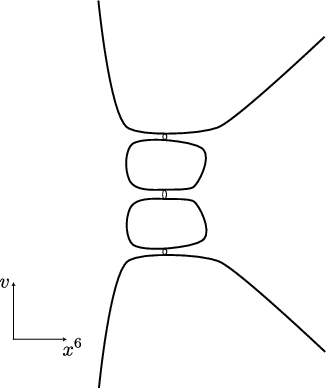
Our classical Type IIA brane configuration is new in the sense that not only but projection yields relatively curved NS5-branes. Besides, using these brane setups, one can easily judge whether it preserves SUSY or not from the intersection of NS5- and D4-branes on -plane. This is illustrated in Figure 4.
We have assumed a linear and a quadratic just as in [1]. The authors there showed that how SUSY and non-SUSY vacua occur according to . The difference between Figure 4 (a) and (b) lies on a displacement along , namely, the value of in (1.3). Naively, the lower stack of D4-branes in Figure 4 (b) acquires a negative bare gauge coupling for as argued in [1]. Rather, this can be interpreted as the presence of anti-branes or, in Type IIB language, the flip of orientations of ’s. When lifted to M-theory such that [16]
| (3.5) |
the above fact then emphasizes that the M5-brane can no more stay supersymmetric due to its non-holomorphic way of embedding with both and . As far as the matrix model spectral curve (2.5) concerned, anti-eigenvalues (holes) dwelling in [17] can be thought of as the appearance of anti-branes in -space, which do not disturb what happen in -space.
By doing so, spontaneously SUSY breaking vacua can be explicitly constructed by means of Type IIA brane configurations like Figure 4. The terminology “SUSY/non-SUSY duality” bears similarity to Seiberg duality because they amount to crossing NS5-branes and thereby changing the coupling constant.
 |
 |
| (a) | (b) |
3.1 effective superpotential
Now, let us see how the effective superpotential gets modified in the presence of . For gauge theory, the M-theory approach to deriving the effective superpotential is initiated by Witten [20]. He suggested the following integral
| (3.6) |
where is a holomorphic three-form. is a three-manifold having two boundaries, i.e. the previously-defined and a reference surface homologous to .
If there exists a two-form which satisfies
| (3.7) |
then (3.6) can be written as
| (3.8) |
where and . Since is physically irrelevant, the effective superpotential reduces to
| (3.9) |
Now, it is straightforward that
| (3.10) |
upon making use of Riemann’s bilinear identity. Here, ’s denote cycles around cuts while ’s are paths connecting and , see Figure 5.

Because near the neighborhood of each cut (: number of D4-branes attached on the cut), one has
| (3.11) |
Next, since integrals over naively diverge, it is necessary to introduce a cut-off scale at for regularization. The integral is nothing but a line integral over the coordinate , that is, it just gives a regularized complex separation between two NS5-branes or the gauge coupling on the compactified D4-brane. Therefore, the bare Yang-Mills coupling constant evaluated at is related to by
| (3.12) |
Plugging these into (3.10), we obtain the effective superpotential ()
| (3.13) |
where the glueball and stand for dual periods in the context of special geometry. With perturbation, from (3.4) we find that (3.10) can be immediately generalized into
| (3.14) |
This reproduces precisely what derived by Aganagic et al. in [1].
3.2 Partial SUSY breaking from to
 |
 |
 | ||
| (a) | (b) | (c) |
Finally, we comment on the partial SUSY breaking from to through the above brane picture. The partial SUSY breaking is discussed in [21, 22, 23] for Abelian gauge group. The non-Abelian generalization is well investigated and established by authors of [24]. According to these early works, theory is firstly perturbed by introducing a general prepotential of the form (1.3) and its SUSY is broken down to thereof upon adding Fayet-Iliopoulos (FI) parameters.
As mentioned throughout this paper, the prepotential describes how NS5-branes get deformed in -space, see Figure 6 (a). Three FI parameters correspond to the relative position of two NS5-branes in -space. Henceforth, turning on FI parameters means that two NS5-branes are separated from each other in -space. In addition, a new direction by which the bare coupling constant is measured should be defined due to the presence of FI parameters. In Figure 6 (a), initial positions of D4-branes are not fixed. But if D4-branes still remain at their initial positions, they become non-parallel when the curved NS5-brane is pulled along , see Figure 6 (b). In other words, SUSY can no longer be maintained for an off-shell choice of vev. To recover SUSY, D4-branes should be re-distributed appropriately at critical loci, i.e. (on-shell condition). Now, since SUSY is recovered to , we can as well recognize the tree-level superpotential as with coefficients rescaled suitably, see Figure 6 (c). To this end, the partial SUSY breaking mechanism can thus be understood pictorially from the extended brane configuration.
The above argument is valid only for the classical (UV) theory. In order to extend this picture to the full quantum theory, we need to replace the NS5/D4 system with a MQCD curve. Pulling out one NS5-brane then corresponds to deforming the curve. The projective information of the MQCD curve contains both the extended SW curve and loop equation (or, alternatively, generalized Konishi anomaly equation) of theory. Therefore, it is interesting to see how these aspects transform according to the partial SUSY breaking deformation of the curve.
4 Conclusion and discussion
So far, we have shown how the SUSY/non-SUSY duality proposed by Aganagic et al. can have a corresponding Type IIA brane picture. Apart from conventional ones, where anti-branes are wrapped on a CY by hand, the setup here involves changing the orientation of local two-cycles through a varying background NS-flux. This dose work because -field gives a Kähler moduli of arbitrary sign to shrinking two-cycles and hence controls their flops. On Type IIA side, we interpret this background as two crossing NS5-branes where -branes appear naturally for flipped orientations. Consequently, simultaneous presence of D4- and -branes soon suggests a way to realize various kinds of SUSY/non-SUSY vacua via adjusting parameters the NS-flux contains. Moreover, curved NS5-branes on -plane with SUSY correspond to what has been known as the Seiberg-Witten theory. One can further add FI parameters to partially break down to . Resorting to Type IIA brane pictures, we see this process is clearly visualized in Figure 6. The final vacuum is arrived at once the tree-level superpotential takes the form of .
We also considered M-theory lift. Without perturbation, the M-theory curve itself is either a degenerated Seiberg-Witten curve on -plane or a loop equation of DV matrix model on -plane. Though adding higher terms has no effect on the planar loop equation, we find that effective superpotential which involves -cycles on -plane gets modified. In particular, it seems that the above partial SUSY breaking process can be described by deforming one given M-theory curve in order to incorporate quantum effects. It is thus of interest to compare this observation with field theory results found in [25]. We leave these problems to future works.
Acknowledgements
We are grateful to K. Hashimoto for helpful discussions. KO would like to thank T. Higaki and K. Maruyoshi for useful comments. KO is supported in part by Grant-in-Aid for Scientific Research (No.19740120) from the Ministry of Education, Culture, Sports, Science and Technology. TST is supported in part by the postdoctoral program at RIKEN.
References
- [1] M. Aganagic, C. Beem, J. Seo and C. Vafa, “Extended Supersymmetric Moduli Space and a SUSY/Non-SUSY Duality,” arXiv:0804.2489 [hep-th]
- [2] M. Aganagic, C. Beem, J. Seo and C. Vafa, “Geometrically induced metastability and holography,” Nucl. Phys. B 789 382 (2008) [arXiv:hep-th/0610249]
- [3] J. Marsano, K. Papadodimas and M. Shigemori, Nucl. Phys. B 789 294 (2008) arXiv:0705.0983 [hep-th]; arXiv:0801.2154 [hep-th]
- [4] M. Aganagic, C. Beem and B. Freivogel, “Geometric Metastability, Quivers and Holography,” Nucl. Phys. B 795 291 (2008) arXiv:0708.0596 [hep-th]
- [5] L. Hollands, J. Marsano, K. Papadodimas and M. Shigemori, “Nonsupersymmetric Flux Vacua and Perturbed N=2 Systems,” arXiv:0804.4006 [hep-th]
- [6] H. Ooguri and Y. Ookouchi, “Meta-stable supersymmetry breaking vacua on intersecting branes,” Phys. Lett. B 641, 323 (2006) [arXiv:hep-th/0607183]
- [7] S. Franco, I. Garcia-Etxebarria and A. M. Uranga, “Non-supersymmetric meta-stable vacua from brane configurations,” JHEP 0701 085 (2007) [arXiv:hep-th/0607218]
- [8] I. Bena, E. Gorbatov, S. Hellerman, N. Seiberg and D. Shih, “A note on (meta)stable brane configurations in MQCD,” JHEP 0611 088 (2006) [arXiv:hep-th/0608157]
- [9] K. Intriligator, N. Seiberg and D. Shih, JHEP 0604, 021 (2006) [arXiv:hep-th/0602239]
- [10] A. Giveon and D. Kutasov, “Brane dynamics and gauge theory,” Rev. Mod. Phys. 71 983 (1999) [arXiv:hep-th/9802067]
- [11] A. Hanany and E. Witten, “Type IIB superstrings, BPS monopoles, and three-dimensional gauge dynamics,” Nucl. Phys. B 492 152 (1997) [arXiv:hep-th/9611230]
- [12] M. Bershadsky, C. Vafa and V. Sadov, “D strings on D manifolds,” Nucl. Phys. B 463 398 (1996) [arXiv:hep-th/9510225]
- [13] H. Ooguri and C. Vafa, “Two-dimensional black hole and singularities of CY manifolds,” Nucl. Phys. B 463 55 (1996) [arXiv:hep-th/9511164]
- [14] A. Karch, D. Lust and D. J. Smith, “Equivalence of geometric engineering and Hanany-Witten via fractional branes,” Nucl. Phys. B 533 348 (1998) [arXiv:hep-th/9803232]
- [15] K. Dasgupta, K. Oh and R. Tatar, “Geometric transition, large N dualities and MQCD dynamics,” Nucl. Phys. B 610 331 (2001) [arXiv:hep-th/0105066]
- [16] E. Witten, “Solutions of four-dimensional field theories via M theory,” Nucl. Phys. B 500 3 (1997) [arXiv:hep-th/9703166]
- [17] R. Dijkgraaf and C. Vafa, Nucl. Phys. B 644 3 (2002) [arXiv:hep-th/0206255]; Nucl. Phys. B 644 21 (2002) [arXiv:hep-th/0207106]; [arXiv:hep-th/0208048]
- [18] F. Cachazo, K. Intriligator, and C. Vafa, “A Large N Duality via a Geometric Transition,” Nucl. Phys. B 603 3 (2001) [arXiv:hep-th/0103067]
- [19] A. Marshakov and N. Nekrasov, “Extended Seiberg-Witten theory and integrable hierarchy,” JHEP 0701 104 (2007) [arXiv:hep-th/0612019]
- [20] E. Witten, “Branes and the dynamics of QCD,” Nucl. Phys. B 507 658 (1997) [arXiv:hep-th/9706109]
- [21] I. Antoniadis, H. Partouche and T. R. Taylor, Phys. Lett. B 372, 83 (1996) [arXiv:hep-th/9512006]; I. Antoniadis and T. R. Taylor, Fortsch. Phys. 44, 487 (1996) [arXiv:hep-th/9604062]
- [22] S. Ferrara, L. Girardello and M. Porrati, Phys. Lett. B 376, 275 (1996) [arXiv:hep-th/9512180]
- [23] H. Partouche and B. Pioline, Nucl. Phys. Proc. Suppl. 56B, 322 (1997) [arXiv:hep-th/9702115]
- [24] K. Fujiwara, H. Itoyama and M. Sakaguchi, Prog. Theor. Phys. 113, 429 (2005) [arXiv:hep-th/0409060]; Nucl. Phys. B 723, 33 (2005) [arXiv:hep-th/0503113]; K. Fujiwara, Nucl. Phys. B 770, 145 (2007) [arXiv:hep-th/0609039]
- [25] H. Itoyama and K. Maruyoshi, Phys. Lett. B 650, 298 (2007) arXiv:0704.1060 [hep-th]; Nucl. Phys. B 796, 246 (2008) arXiv:0710.4377 [hep-th]