Sagnac interference in Carbon nanotubes
Abstract
The Sagnac interference mode arises when two interfering counterpropogating beams traverse a loop, but with their velocities detuned by a small amount , with . In this paper we perform a perturbative non-equilibrium calculation of Sagnac interference in single channel wires as well as armchair nanotube loops. We study the dependence of the Sagnac conductance oscillations on temperature and interactions. We find that the Sagnac interference is not destroyed by strong interactions, but becomes weakly dependent on the velocity detuning . In armchairs nanotubes with typical interaction strength, , we find that the necessary temperature for observing the interference effect, is also only weakly dependent on the interaction, and is enhanced by a factor of 8 relative to the temperature necessary for observing Fabry-Perot interference in the same system, .
I Introduction
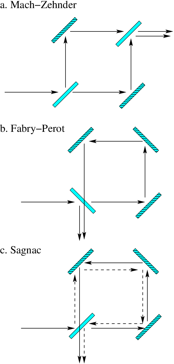
One of the most tantalizing effects predicted by quantum mechanics is the appearance of interference fringes when two matter beams come together. These fringes provided the ultimate testimony to the pertinence of quantum mechanics and the Schrödinger equation. Interferometry of light is employed in many precision measurement devices. The Mach-Zehnder interferometer produces interference between two beams traversing two distinct paths, one of which passes through a test chamber containing, for instance, a dilute gas (see Fig.1); this setup was originally used to measure the refraction index of the gas in the chamber. Fabry-Perot interferometer recombines a series of beams, where the n’th beam traverses the optical path between two mirrors or through a loop times. The narrowness of the resulting interference peaks allows a precise measurement of a light beam’s wave length, and is commonly used to measure the Zeeman splitting of an atom in a magnetic field. The most sensitive of all interference constructs, however, is the Sagnac interference[1]. In this setup, a light beam is split into two beams, which traverse the interferometer’s loop both clock wise and counter clock wise, before being recombined. In this case, the interference fringes arise due to an absolute rotation, and provide the most accurate measure of the angular velocity of the device. This was used by Michelson to measure the absolute rotation of the Earth. More recently, the Sagnac interference effect was cleverly used to measure time reversal symmetry breaking in superconductors [2].
Quantum mechanics opened the way for matter-wave interferometry. Electron interferometry is a powerful probe of interaction effects on low-energy phases of quantum matter, as demonstrated by numerous examples. Mach-Zehnder interferometers reveal Aharonov-Bohm oscillations and quantum hall effect edge channels[3, 4, 5, 6, 7], and can probe exotic fractional quantum Hall states[8, 9, 10]. Similarly, two-path Mach-Zehnder interferometers can probe correlated states of quantum dots[11, 12]. Of particular interest to us are metallic carbon nanotubes. The Luttinger liquid behavior in these systems[13, 14, 15] was partially verified through the observation of Fabry-Perot interference in finite sections of the nano-tube [16]. The Fabry-Perot interference should, in principle, allow the observation of spin-charge separation and determination of the interaction parameters of the Luttinger liquid [17]. But the similar energy scales of the spin and charge modes’ interference patterns has made such experimental observation challenging.
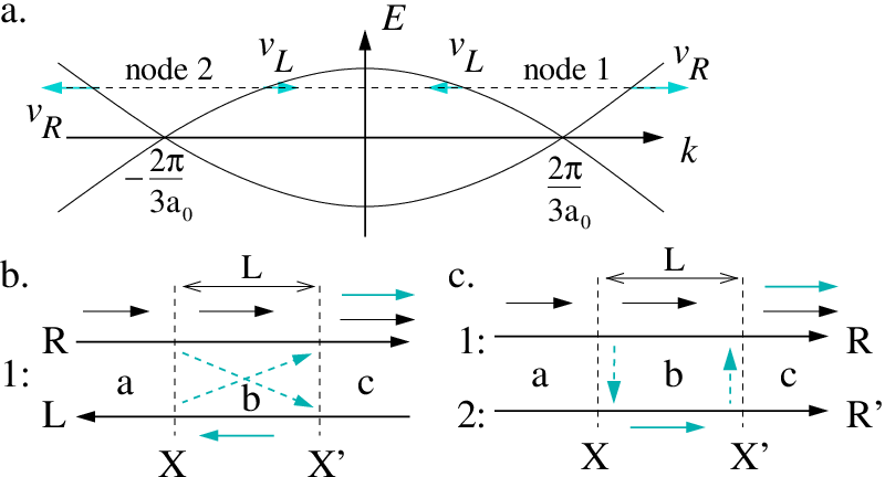
The most sensitive interferometer of all, however, the Sagnac interferometer, has not been seriously explored yet in the context of interacting electronic systems. In Ref. 18 we proposed that this interference naturally occurs in metallic armchair nanotube loops (Fig. 2). Instead of rotation, the Sagnac interference arises due to the band velocity difference between right- and left-moving electrons about each Dirac node. This velocity difference is present whenever the electronic Fermi surface is tuned away from the Dirac points at half-filling, as shown in Fig. 3(a). The operating principle of the electronic Sagnac effect has the same origin as the universal conductance fluctuations, and weak-localization effects in disordered two-dimensional electron gases [19, 20, 21]. In nanotubes, it can also appear due to band-scattering in a pair of impurities [22].
Because the Sagnac effect involves electrons traversing the same path in two different directions, rather than repeating the same path as in Fabry-Perot interference, the phase accumulation is extremely small. Therefore Sagnac interference exhibits large-period conductance fluctuations as a function of gate- and source-drain voltages, and is expected to persist to high temperatures in comparison to Fabry-Perot interference, which is more sensitive to thermal dephasing. This interference mode should thus be able to reveal much more precise information about the unique state of interacting electrons in thin quantum wires.
Our goal in this manuscript is to thoroughly explore the range and robustness of the Sagnac interference mode, concentrating on armchair Carbon nanotubes. The questions we will ask concern the amplitude of this interference mode as a function of the temperature, gate and source-drain voltage, and Luttinger parameter of the nanotube.
The paper is organized as follows. In Section II, as a warm-up, we analyze the simpler case of Sagnac interference in a single channel of right- and left-moving electrons. In II.1 we introduce the model of a single channel with a linearized spectrum, and the cross-loop tunneling which will give rise to the Sagnac interference. In II.2 and II.3 we set up the non-equilibrium perturbative calculation of the conductance in the presence of cross-loop tunneling, and in II.4 and II.5 we analyze the behavior of the oscillating conductance as a function of gate and bias voltages and temperature. In Section III we repeat the above steps for the physically relevant case of Carbon nanotubes, including spin and node degeneracies in the calculation, and remark on the similarities and differences from the single channel case. Finally we conclude with a discussion of the experimental implications of our calculations.

II Sagnac interference in a single channel
As discussed in the introduction, the Sagnac interference in the loop geometry is due the the asymmetry between the velocities of the left and right moving electrons. To demonstrate this in the simplest form, we first study in this section a single channel with a single type of left and right movers. In a carbon nanotube, there will be four such channels due to spin and node degeneracies.
II.1 The Model
We start with a single one dimensional channel of electrons and a linearized spectrum, with different left and right mover velocities, and a density-density interaction. The Hamiltonian density for this system is:
| (1) |
where the operator creates a right/left moving electron, with the velocity:
| (2) |
The scattering we are interested in is the one which takes a right moving electron at one side of the loop, point is Figure 2, and scatters it to a left moving electron at the other side of the loop, point , and vice versa. This process has been dubbed Cross-Loop scattering in Ref. [18]. The same effect can also be obtained without the loop geometry by inter-node tunneling [22], since right movers at node move with the same velocity as left movers at node . This inter-node tunneling is shown in Figure 3(c). If we choose our coordinate along the loop such that the point corresponds to and the point corresponds to , then this scattering process is described by the Hamiltonian:
| (3) |
In the presence of the quartic density-density interactions in the Hamiltonian, Eq. (1), it is useful to use the standard bosonization procedure , since the Hamiltonian is quadratic in terms of the bosonic fields. The electron fields are bosonized as follows:
| (4) |
where and are bosonic fields that satisfy the commutation relations ; also, the total density and the current density are given by , and , respectively. The Hamiltonian in terms of the bosonic fields becomes:
| (5) |
where is the Luttinger interaction parameter and . This is the familiar Hamiltonian of a 1D interacting electron system, with the addition of the term which gives left and right moving particles different velocities. Indeed, this Hamiltonian can be easily diagonalized and the left and right velocities turn out to be for a general value of the interaction parameter :
| (6) |
Our goal is to calculate the effects of the Sagnac interference as seen in the conductance as a function of the applied bias and gate voltages, and as a function of temperature. Due to the applied voltages the system is not in equilibrium, and we must turn to the Keldysh non-equilibrium formalism [23, 24]. Below we carry out this analysis first for the simplified electron gas with the scattering Hamiltonian , Eq. (3), as a perturbation.
II.2 Non-Equilibrium correlation functions and conductance
The response of the loop to a bias source-drain voltage can be analyzed using the non-equilibrium Keldysh formalism. Following Ref.17, we assume that in the distant past, before turning on the backscattering, the left and right moving electrons separately had well defined thermal distributions set by separate chemical potentials. The density matrix corresponding to this initial distribution at temperature is:
| (7) |
with and the Hamiltonian which takes into account the applied voltages is:
| (8) |
The gate voltage, , simply couples to the total charge density, with being a geometrical factor of the system, while the source-drain voltage, , induces the imbalance in the chemical potentials of the left and right movers.
As explained in Ref. 17, both and can be eliminated from the unperturbed action by an appropriate unitary transformation, which is equivalent to shifting the bosonic fields by a function of space and time; this is easy to see if one writes down the Lagrangian including the voltages[18]. The equivalent shifts for the case at hand are:
| (9) |
These shifts remove the voltages from the Hamiltonian and therefore all the correlations to appear in the calculation will be equilibrium correlation functions with respect to . The dependance on the applied voltages now appears in the scattering Hamiltonian, , due to the shifted bosonic fields.
Let us now focus our attention at the charge current, which in the bosonic language is . After performing the unitary transformation described above we can write the formal expression for the expectation value of the current in the usual interaction picture [17]:
| (10) |

is the time ordering operator along the Keldysh contour shown in Fig.4, and is the symmetrized current operator with respect to the two branches of the contour. The current is the ideal current that would flow in the absence of backscattering in a completely transmitting channel, and it explicitly appears due to the shift of the field. The Hamiltonian denotes the scattering Hamiltonian with the properly shifted bosonic fields. The expression for the current can be expanded in powers of , and all the correlation functions to appear in this expansion are equilibrium correlation functions at temperature . If we denote by and the fields on the forward branch and backward branch of the Keldysh contour respectively, then time ordering along the contour means that correlations have the usual time ordering, are anti-time ordered, and is always earlier in time that . The same applies for all the fields.
It is useful to apply a Keldysh rotation to the fields, , and similarly for . The correlation function vanishes by construction, and we define :
| (11) |
and similarly for the fields, and for the mixed correlations:
| (12) |
where operators with a hat are simply the time dependent operators with no time ordering. As explained above, these correlation function are to be evaluated in equilibrium, and therefore are easily explicitly calculated (Appendix B). Due to translational invariance in time and space, these correlations are functions of and , for example:
| (13) |
II.3 Perturbation Theory
The Sagnac interference fringes occur already with weak bakcscattering at the base of the loop, and can be deduced from a perturbation analysis of the tunneling Hamiltonian, Eq. (3). As outlined above, to calculate the current, , we absorb the gate and bias voltages, and respectively, in the shifts in Eq.9, which allow us to move the voltages from the unperturbed Hamiltonian to the backscattering perturbation, . Then, we expand the formal expression we found for the current using the Keldysh technique, Eq. 10, in powers of , and use Wick’s theorem to evaluate the resulting contributions.
To lowest nontrivial order, which is second order in , we obtain after a lengthy calculation:
| (14) |
The first term is simply the current that would flow through the system in the absence of backscattering. The coherent current, , oscillates with the gate voltages , and is given by:
| (15) |
where c is a constant of order unity, and we assume that are real for simplicity. The incoherent current, , is independent of the gate voltage, and is given by:
| (16) |
The functions , , and are complicated combinations of the correlation functions defined in section II.2 and are given explicitly in Appendix B. These functions do not simplify, partly due to the fact that the correlation functions in this problem are not symmetric under since left and right movers have different velocities.
II.4 Voltage dependence of the single-mode Sagnac interference
The voltage current characteristics given in Eqs. (14 - 16) can be evaluated numerically to obtain the voltage and temperature dependence of the single-mode Sagnac interference. The period of the interference as a function of the gate voltage () are easily observed to be (for small ):
| (17) |
where is the period in gate voltage for Fabry-Perot interference. Fabry-Perot interference occurs whenever part of the wave’s trajectory can be repeated. Since the Sagnac interference involves traversing the same path in two different directions, the phase difference accumulated in the process is much smaller than the difference incurred by repeating part of the path, and therefore the period of the Sagnac interference is much larger than the period of the Fabry-Perot interference. Such large period oscillations have been experimentally observed in Carbon nanotubes, in the loop geometry, as reported in Ref.18, in addition to the shorter period Fabry-Perot oscillations.

For a given gate voltage, both the coherent and incoherent parts of the current oscillate with the bias voltage . This oscillation is due to the fact that in the presence of bias voltage, the Fermi energy of the left- and right- moving electrons are different by , and hence their Fermi wavevectors are different also and they would acquire different phases traversing the loop. This oscillation will be present even for no velocity detuning, . When the detuning is finite, , the differential conductance will show a beating pattern due to the two different left and right moving excitation velocities. Here we are only considering the Sagnac oscillations arising from the cross-loop tunneling, Eq. (3). Figure 5 shows the oscillations of the differential conductance at a fixed gate voltage. For non-interacting electrons, the beating pattern corresponds to the addition of two harmonics with two different frequencies in voltage, and , with and . The beating pattern will then display fast oscillations with voltage period , and slow voltage oscillations with period . For interacting fermions, , the oscillations will not be simple harmonic oscillations. Still, the periods will be evident and will have the same functional form, in terms of , as the frequencies in the non-interacting case. The periods and do depend on through velocities and , (Eq. 6).
These oscillation, generally, lie atop a powerlaw behavior of the differential conductance as a function of , as expected from the known behavior of the conductance in the presence of impurity backscattering [25]. For backscattering from an impurity in a Luttinger liquid, the backscattered current, for low temperature, behaves as . We chose to plot the Sagnac oscillations as a function of (Fig. 5) for the interaction parameter since for that value the corresponding power law would be , and the contribution of such a powerlaw to the differential conductance would vanish, making the oscillation atop this powerlaw more visible.
II.5 Temperature dependence of the single-mode Sagnac interference
Next we consider the temperature dependence of the gate-voltage driven oscillations in the coherent part of the current. As argued in Ref. 18, the large period Sagnac oscillations are expected to be observed at much higher temperature than the shorter period Fabry-Perot oscillations. This difference in temperature behavior can be easily understood by examining the phase giving rise to the interference in both cases. In the Fabry-Perot case for a loop, the lowest order interference is between a beam of electrons which is not scattered, and a beam of electrons which, due to scattering at the base of the loop, does a roundtrip between the the two scattering points. The phase difference between these two beams at energy is . Finite temperature effectively causes uncertainty of order in the energy , and the interference pattern will be washed out when the uncertainty of the the phase is of order , which happens at a temperature .
In the Sagnac case, the interference is between a beam that traverses the loop moving left and one which traverses the loop moving right. The phase difference between these two beams at energy is , and this interference will be washed out at temperature . For non-interacting electrons the right and left moving velocities are . Thus to lowest order in , the highest temperatures for observing interference according to the argument above are:
| (18) |
For non-interacting electrons, we expect the Sagnac interference to survive to a temperature higher by a factor of than the corresponding Fabry-Perot temperature. We will show through explicit calculation that this is indeed true for the non-interacting case. For interacting electrons, we will see that will still be considerably larger than , but their ratio is less than the dramatic ratio.
To explore the Sagnac temperature range, we evaluate the amplitude of the coherent oscillations (the oscillations in ) as a function of temperature, for different interaction parameters and different ratios of . For non-interacting electrons, , we find that the Sagnac oscillations indeed survive up to a high temperature, which is a factor of higher than the corresponding Fabry-Perot oscillations. Figure 6 plots the oscillation amplitude as a function of temperature, normalized by its zero-temperature value, and for different values of . The functional dependence on temperature is given approximately by:
| (19) |
This result is similar to the exact form of the temperature dependence of the Fabry-Perot interference amplitude [26], with the only difference being the factor of . Therefore, the Sagnac oscillations of non-interacting electrons indeed survive up to a temperatures which are a factor of larger than the Fabry-Perot oscillations.

For interacting electrons, , the Sagnac interference still survives up to temperatures significantly higher than the corresponding Fabry-Perot temperature scales, but the enhancement is suppressed compared to that of non-interacting electrons. Figure 7 shows the Sagnac temperature scale vs. for three different values of the interaction parameter , where we define to be the temperature at which the amplitude of the oscillations reaches of its amplitude at zero temperature. For non-interacting electrons is strongly dependent on the ratio as discussed above. For the interaction parameter values and (Dashed lines), the temperature is only weakly dependent on the ratio . As an example for the resulting enhancement of the Sagnac compared to the Fabry Perot interference, consider , where the temperature scale for the Sagnac oscillations is roughly , a factor of 4 enhancement over of the non-interacting Fabry-Perot oscillations which is , despite the suppression of the Sagnac due to interactions. As can be seen in the figure, for the enhancement is about 7. While it is difficult to extract the analytic dependence of the temperature on the interaction parameter, one can repeat our calculation for any value of .

III Interference in Nanotubes
Equipped with our understanding of the single-channel Sagnac interference, we can now consider the likely physical system where it may be observed: a metallic Carbon nanotube with four different Dirac nodes. We now add the spin and node degeneracies of a Carbon nanotube, and examine their effect on the Sagnac interference pattern voltage and temperature dependence.
III.1 The Model
The energy spectrum of a Carbon nanotube is shown in figure 3 a. This spectrum is usually linearized around the Fermi surface, which yields four chiral modes, two left moving and two right moving (not including spin), with linear dispersion. These modes can be bosonized and treated within the Luttinger Liquid theory framework, as we have done in the single channel case in the previous sections. All these modes are usually assumed to have the same velocity, the Fermi velocity . For the purposes of this paper, it is important to notice that when the Fermi surface is away from the degeneracy points where the upper and lower bands meet, linearizing the spectrum actually gives two different velocities which we shall note . The linearized Hamiltonian density is, then:
| (20) |
where stands for a right/left moving electron at node with spin , and we added a total charge density interaction term. The velocities that appear in the Hamiltonian are:
| (21) |
Thus for , at node right movers are faster than left movers, while at node the opposite is true. Now, the nonlinearity of the elctronic spectrum in a Carbon nanotube needs to be taken into account when considering the velocity difference, ; it depends on the detuning of the chemical potential away from the degeneracy points.
The scattering process we are interested in is very similar to the one we had in the single channel case. We need to consider a term that scatters a right mover at one end of the loop to a left mover at the other end of the loop, conserving spin and node quantum numbers,
| (22) |
Next we bosonize the electron field operators in the nanotube. The slowly oscillating parts can be written as:
| (23) |
where and are bosonic fields that satisfy the commutation relations . The Hamiltonian in terms of the bosonic fields is [18]:
| (24) |
If the velocities of all branches of the spectrum were equal, i.e. , then the Hamiltonian would be diagonalized by the spin and node symmetric and antisymmetric combinations of the ’s and ’s [14]. By diagonalizing we mean a linear mapping of the and fields such that the Hamiltonian takes the form of four independent channels, each resembling of , Eq. (5). When , there still exists a local transformation that diagonalizes the Hamiltonian, but it is a more complicated combination of the fields that depends on and , and mixes the and fields, which makes the conductance calculation quite cumbersome. While the details of this transformation are given in appendix A, the diagonal Hamiltonian is:
| (25) |
The fields and are the spin antisymmetric combinations of and respectively. Since the interaction term in Eq.(20) involves only the spin symmetric combinations, the spin antisymmetric combinations are untouched and still have the left and right moving velocities as in Eq.(21). On the other hand, the fields and are not simply the remaining symmetric combination and mix the remaining ’s and ’s. These fields have the same left and right moving velocity, which is:
| (26) |
where is the Luttinger parameter.[27]
Fortunately, for the region of parameters which is of interest, namely strong interactions, and , the exact change of basis required to diagonalize the spin symmetric part of the Hamiltonian is very close to the usual node symmetric/antisymetric basis. This can be explicitly seen, for example, from the velocities of these modes. For this entire range of parameters, the velocities of the diagonal fields, given by Eq.(26), are at most different from the values we expect for the left-right symmetric system, which are and . Due to the strong interactions in this spin symmetric sector, the velocity asymmetry is unimportant, and it is for this reason that we choose to still use the node symmetric-antisymmetric basis and treat these fields as the diagonal ones. In Appendix A we elaborate on and justify this approximation. Note that the velocity asymmetry is still apparent in the non-interacting spin antisymmetric modes labeled by and in Eq. (25).
III.2 Perturbation Theory
Using the diagonal form of the Hamiltonian with the above approximation, we proceed to calculate the current, , as in Section II. The applied voltages now couple to the total density and total number of left movers and right movers:
| (27) |
The external voltages can be removed from the Hamiltonian by the appropriate shift of the bosonic fields:
| (28) |
Again we use the Keldysh contour to write the formal expression for the current, as in Eq. (10), and expand it to lowest order in the appropriate which contains the voltage dependence due to the shifts of the fields. The approximation we made above, namely that it is the node symmetric/antisymmetric combination which diagonalize the Hamiltonian, allows us to write the current in a very similar form to the single channel case:
| (29) |
The first term on the right hand side of Eq. (29 is the current that would flow in the nanotube in the absence of backscattering. The second term is the coherent current which oscillates with the gate voltage:
| (30) |
and the third term is the incoherent current, which is independent of the gate voltage:
| (31) |
The function , , and are related to the single channel correlation functions as explained in Appendix B.

III.3 Temperature and Voltage Dependence in Carbon Nanotubes
As in the single channel case, we find there is a coherent part of the interference current which oscillates as a function of the gate voltage with a large period, much larger than the Fabry-Perot oscillation period, as seen explicitly from the voltage dependence of .
The differential conductance , on the other hand, displays a beating pattern, but a more complicated one than in the single-channel case, since there are four different velocities in the problem now: , and . Figure 8 shows the differential conductance of the nanotube, , and its Fourier transform. From the Fourier analysis we see that clearly there are four dominant frequencies, which correspond to the four different velocities of the collective modes in the nanotube. Thus a careful observation of the large-period, and robust, Sangac interference allows, in principle, to extract the nanotube parameters, namely the interaction strength and the velocity mismatch from the Fourier transform of the conductance as a function of bias voltage, up to temperatures much higher than the Fabry-Perot oscillations temperatures.
The temperature dependence of the Sagnac interference in the nanotube case is qualitatively similar to the single channel case. In the absence of interactions (), the interference can be observed to the scale proportional to ; in the presence of strong interactions, however, becomes only weakly dependent on . Unlike the single channel case, in the nanotube case is also only very weakly dependent on in the range . This is due to the fact that only one of the four modes which diagonalize the Hamiltonian are interacting and depend on . For the same reason, is higher in the case of the nanotube than in the single channel case, i.e. the reduction of due to interactions is not as severe in the nanotube case. The temperature dependence on and is plotted in Figure 7. In the range mentioned above, .
IV Summary and Conclusions
In this paper we investigated the conductance oscillations in carbon nanotubes due to Sagnac interference. In addition to theoretical interest in this large-period interference mode, the motivation for our study also comes from a recent experimental realization of carbon nanotube loops [18]. The same interference mode can arise also without the loop geometry in the presence of internode backscattering in the nanotube, as pointed out in Ref. 22.
The source of the Sagnac conductance oscillations is the difference in the velocities of left and right moving excitations in a carbon nanotube when the chemical potential is tuned away from half filling. Compared to the more familiar Fabry-Perot oscillations [16], Sagnac oscillations are expected to have a much larger period in gate voltage, and, as we show, in non-interacting wires survive to a temperature a factor of higher than that required to observe Fabry-Perot oscillations.
In interacting electronic wires, the above temperature estimation for free fermions does not apply. Our results for a single channel Luttinger liquid are that becomes only weakly dependent on , although still strongly dependent on . From our results, the enhancement of relative to the FP interference is roughly: in the range .
For a strongly interacting armchair nanotube, , we find that becomes not only weakly dependent on , but also nearly independent of . The Sagnac interference is expected to survive upto . Considering that Fabry-Perot oscillations have been observed in nanotubes up to [16], Sagnac oscillations should be observed up to about in nanotubes, despite the strong interactions.
There is also something to be learnt from examining the behavior of the conductance as a function of the applied voltages. We saw that Sagnac oscillations would have a large period of oscillations in the applied gate voltage ; this period itself is a function of the gate voltage, through the dependence of the velocity difference . Using typical values of a nanotube parameters (e.g. Ref. 18), , , and , the period of oscillation in the gate voltage would be , consistent with the observed oscillations in Ref. 18.
On the other hand, oscillations of the conductance as a function of the applied bias voltage depend not only on the bare velocities, but also on the interaction strength. A Fourier transform of the Sagnac oscillations as a function of , we show, contains four different frequencies corresponding to the four different velocities in the problem, which are roughly , and . Using the same parameters as above we get . This period is much smaller than the bandwidth of a nanotube which is a few eV, so in principle many oscillation periods can be observed and the longer period oscillations should also be measurable, allowing the slower frequency oscillations to appear in the Fourier transform. Observation of these frequencies would allow us to read off the parameters of the nanotube, , and , at temperatures up to , which is higher than the temperatures associated with Fabry-Perot oscillations.
In the single channel case, for non-interacting electrons, we were able to extract an analytic expression for the temperature behavior of the conductance gate voltage oscillations :
| (32) |
and it is apparent how the ratio directly enters the temperature scale. Unfortunately, we were so far unable to extract analytic expression for in terms of and for the interacting single channel or interacting nanotube cases, inspite of the progress on the qualitative understanding our numerical results allow. Such an analytical understanding should be the focus of a future effort.
As can be observed in Figs. 1 and 2, the paths giving rise to the Sagnac intereference are similar to the paths that give rise to weak localization phenomena in 2d disordered conductors. In this work we also essentially show that even in the presence of strong interactions, the interference survives. It is tempting to extrapolate from our results that weak localization should also survive strong interactions. This, however, is presumably true so long that scattering events are dominated by small momentum transfer. Nevertheless, our results suggest that a Luttinger liquid with charge and spin modes will still exhibit weak-localization effects, but suppressed, and only weakly dependent on the detuning between counter propogating electrons. Therefore the magnetoresistance should also be strongly suppressed at low fields.
Acknowledgements.
We are indebted to Jinseong Hu, Chetan Nayak, Yuval Oreg, Leonid Pryadko, and Jan von Delft for illuminating discussions. MB is grateful for support by the ONR.Appendix A Diagonalizing the Hamiltonian with Node and Spin Degeneracies
In this appendix we show how to diagonalize the Hamiltonian of Eq. (24), where diagonalizing entails finding the appropriate change of basis that will transform to the sum of four Hamiltonians, each having a form resembling the single channel of Eq. (5). We also explain here the approximations we have used in our calculation.
The first step in the diagonalization of is to change the basis from the spin up/down to the spin symmetric/antisymmetic basis at each node:
| (33) |
applying the same transformation to the ’s as well. We notice that the density-density interaction term involves only the spin symmetric fields , hence the spin antisymmetric fields decouple and appear as two non-interacting () copies of the single channel problem, described by the Hamiltonian , with right moving velocity of and left moving velocities of . These are the fields labeled with and in Eq. (25).
The Hamiltonian for the spin symmetric fields has a similar form to our starting point Hamiltonian, :
| (34) | ||||
In the absence of the term, is easily diagonalized by taking the node symmetric and antisymmetric combinations of the fields:
| (35) |
The resulting diagonal Hamiltonian would be:
| (36) |
with , , and .
When we consider , it is still possible to apply a and dependent transformation to the fields, that will restore to the form in Eq. (36), with velocities given by Eq. (26). The field mixing this transformation entails, however, considerably complicates the book keeping in our perturbative calculation. Fortunately, we can show that a good approximation is to simply set to zero in when the interactions are strong, and simply use the transformation given by Eq. (35). The first indication that this approximation is valid is that the exact velocities differ from the velocities by at most in the entire range of parameters we are interested in, which is and
Another indication that this approximation is valid comes from the analysis of the single channel problem in Section II. In the single channel case we derived exact expressions for the Sagnac interference, and found that for and , the temperature dependence is only weakly dependent on ; furthermore only enters directly in the expression for the oscillation period of the conductance as a function of gate voltage, the dependence we have explicitly in our expression for the coherent current , Eq. 15.
Finally, we can also calculate the exact combination of fields that diagonalizes , and verify that indeed they are very close to the node symmetric/antisymmetric combinations for the range of and of interest. As an example, the explicit change of basis from the node symmetric/antisymmetric basis to the diagonalizing basis for , to second order in , is:
We see that the is matrix is close to the identity matrix , since . The deviation from the identity becomes even smaller for smaller . Note that for the corresponding change of basis matrix is not close to the identity matrix and our approximation fails.
We stress that setting to zero in is simply a good numerical approximation which simplifies the calculation, and not equivalent to setting to zero in the entire problem, as still appears in spin anti-symmetric part of the Hamiltonian (where ), and also in the gate voltage dependence.
Appendix B Correlation functions
Let us now connect the explicit expressions for the coherent and incoherent currents given in Section II.3 and Section III, Equations (15) and (16), using the correlation functions defined in Section II.2.
It is useful to define the following combination of :
| (41) |
and similarly for .
In the single channel case discussed in Section II, there are only a single field and a single field, with the Hamiltonian given by Eq.(5). Since the Hamiltonian is quadratic we can easily evaluate all the equilibrium correlation functions at finite temperature, paying attention to the different time orderings that appear as a result of the two branches of the Keldysh contour. The results for finite temperature is:
| (42) | ||||
| (43) |
where is a short distance cutoff, , and is the step function. As mentioned in Ref. 26, it is important to remember that the step functions are not infinitely sharp, and have a transition width of order , the cutoff. The functions and are obtained from and by replacing the prefactor with . The function is given in Eq. (12), and:
| (44) | ||||
The currents are expressed in integrals over complicated combinations of such correlation functions. For example, the coherent part of the current, given by Eq. (15), involves the following combinations:
| (45) | ||||
and
| (46) | ||||
The corresponding functions for the incoherent current are :
| (47) | ||||
and
In a Carbon nanotube there are four channels, rather than a single one. In the non-interacting case, , all these channels are independent and we would recover the results of the single channel. Equations (45) and (46) still apply for this case. When , the different channels are coupled through the interaction, and we must find the correct combinations of the fields and which decouple and therefore diagonalize the Hamiltonian. These combinations are discussed in Appendix A. This change of basis is in general a function of and , and it mixes the and fields, which in turn complicates the functions and further. Luckily, the interactions in Carbon nanotubes are strong, , and in that range, the change of basis is very close to the usual spin/node symmetric/antisymmetric change of basis. If we approximate the diagonalizing fields by these symmetric/antisymmetric combinations, then equations (45) and (46) would apply provided we make the following substitutions:
| (48) |
Where each has a different set of values for , and to be used in Eq.(42). The fields and correspond to the spin asymmetric combinations, which decouple from the interaction, and hence have , and velocities and . The fields and both have the same left and right mover velocities, and respectively, given by Eq. (26), and interaction parameters and , respectively.
References
- [1] G. Sagnac, Comptes Rendus de l’Academie des Sciences (Paris) 157, 708 (1913).
- [2] J. Xia, E. Schemm, G. Deutscher, S. A. Kivelson, D. A. Bonn, W. N. Hardy, R. Liang, W. Siemons, G. Koster, M. M. Fejer, and A. Kapitulnik, Phys. Rev. Lett. 100, 127002 (2008).
- [3] H. Förster, S. Pilgram, and M. Büttiker, Phys. Rev. B 72, 075301 (2005).
- [4] F. E. Camino, W. Zhou, and V. J. Goldman, Phys. Rev. B 72, 155313 (2005).
- [5] W. G. van der Wiel, Y. V. Nazarov, S. De Franceschi, T. Fujisawa, J. M. Elzerman, E. W. G. M. Huizeling, S. Tarucha, and L. P. Kouwenhoven, Phys. Rev. B 67, 033307 (2003).
- [6] B. J. van Wees, L. P. Kouwenhoven, C. J. P. M. Harmans, J. G. Williamson, C. E. Timmering, M. E. I. Broekaart, C. T. Foxon, and J. J. Harris, Phys. Rev. Lett. 62, 2523 (1989).
- [7] E. Buks, R. Schuster, M. Heiblum, D. Mahalu, and V. Umansky, Nature 391, 871 (1998).
- [8] D. E. Feldman and A. Kitaev, Phys. Rev. Lett. 97, 186803 (2006).
- [9] A. Stern and B. I. Halperin, Phys. Rev. Lett. 96, 016802 (2006).
- [10] P. Bonderson, A. Kitaev, and K. Shtengel, Phys. Rev. Lett. 96, 016803 (2006).
- [11] M. Sigrist, T. Ihn, K. Ensslin, M. Reinwald, and W. Wegscheider, Phys. Rev. Lett. 98, 036805 (2007).
- [12] A. Yacoby, M. Heiblum, D. Mahalu, and H. Shtrikman, Phys. Rev. Lett. 74, 4047 (1995).
- [13] M. Bockrath, D. H. Cobden, J. Lu, A. G. Rinzler, R. E. Smalley, L. Balents, and P. L. McEuen, Nature 397, 598 (1999).
- [14] C. Kane, L. Balents, and M. P. A. Fisher, Phys. Rev. Lett. 79, 5086 (1997).
- [15] Z. Yao, H. W. C. Postma, L. Balents, and C. Dekker, Nature 402, 273 (1999).
- [16] W. Liang, M. Bockrath, D. Bozovic, J. H. Hafner, M. Tinkham, and H. Park, Nature 411, 665 (2001).
- [17] C. S. Peça, L. Balents, and K. J. Wiese, Phys. Rev. B 68, 205423 (2003).
- [18] G. Refael, J. Heo, and M. Bockrath, Phys. Rev. Lett. 98, 246803 (2007).
- [19] E. Abrahams, P. W. Anderson, D. C. Licciardello, and T. V. Ramakrishnan, Phys. Rev. Lett. 42, 673 (1979).
- [20] L. P. Gor’kov, D. Khmel’nitzkii, and A. I. 30 248 (1979). Larkin, Pis’ma Zh. Eksp. Teor. Fiz. 30, 248 (1979).
- [21] B. L. Altshuler, A. G. Aronov, and P. A. Lee, Phys. Rev. Lett. 44, 1288 (1980).
- [22] J. Jiang, J. Dong, and D. Y. Xing, Phys. Rev. Lett. 91, 056802 (2003).
- [23] L. V. Keldysh, Zh. Eksp. Teor. Fiz. 47, 1515 (1964), Sov. Phys. JETP 20, 1018 (1965).
- [24] J. Rammer and H. Smith, Rev. Mod. Phys. 58, 323 (1986).
- [25] C. L. Kane and M. P. A. Fisher, Phys. Rev. B 46, 15233 (1992).
- [26] P. Recher, N. Y. Kim, and Y. Yamamoto, Phys. Rev. B 74, 235438 (2006).
- [27] Y. Oreg and A. M. Finkel’stein, Phys. Rev. Lett. 74, 3668 (1995).