How Do Schrödinger’s Cats Die?
How Do Schrödinger’s Cats Die?
Abstract
Recent experiments with superconducting qubits are motivated by the goal of fabricating a quantum computer, but at the same time they illuminate the more fundamental aspects of quantum mechanics. In this paper we analyze the physics of switching current measurements from the point of view of macroscopic quantum mechanics.
PACS numbers: 03.65.Ta, 03.65.Xp, 85.25.Cp, 03.67.Lx
1 INTRODUCTION
Since its very inception, quantum mechanics has defied our classical intuition. Quantum-mechanical correlations established between parts of a system during interaction are of a different nature than the classical ones.[1] Much work has been put recently into harnessing the power of these correlations for performing computational tasks which are very difficult to implement on classical computers. Superconducting qubits based on the Josephson effect have been proposed[2] as the elements of future quantum computers, based on the previously demonstrated macroscopic quantum coherence effects in charge and flux devices.[3]
A number of superconducting qubits are currently under close experimental investigation, such as charge qubits[4], phase qubits[5], flux qubits[6], and a mixed charge-flux version called Quantronium.[7] Quantronium has a very large decoherence time (more than 500ns), and it will be often referred to in the last part of this paper. To measure the qubit, a now standard technique[8] is to monitor the switching probability of a large read-out junction or dcSQUID to which the qubit is coupled. The switching probability depends on the state of the qubit, therefore a change in this probability at the same constant bias current indicates a different qubit state.
If and when a quantum computer can be operated is an open question that depends on the progress in reducing decoherence; even if if will be constructed, a quantum computer will be able to address only a limited number of niche problems - such as factorization and database search - better than its classical counterpart. At the same time, the physics and technology behind present-day qubits is sound, and one may wonder whether these systems will have other potentially interesting applications besides quantum computing. Already technologies based on the properties of entangled light are at a mature stage, leading to industrial applications, e.g. quantum cryptography. At the same time, fundamental research such as testing quantum mechanics at the macroscopic level is an important topic envisioned decades ago[9], with progress in this direction enjoying now a firm experimental basis. The most spectacular test would be a clear experimental proof of violation of Bell’s inequalities, which from the experimental point of view looks like a formidable task ahead of us requiring longer two-qubit decoherence times and read-out systems with a higher visibility than what is currently available. Also, in a more general sense, quantum computing can be regarded as a test of quantum mechanics.
2 THE JOSEPHSON EFFECT
An underdamped Josephson junction[10] can be described by the Hamiltonian
| (1) |
where is the value of the bias current, Gcm2 is the ”barred” flux quanta, is the phase difference of the superconducting order parameter across the junction, is the Josephson energy ( is the critical current), and is the capacitance of the junction. This last electrostatic parameter is conveniently characterized by the energy associated with charging the junction capacitor with a single Cooper pair, . The dynamics of the junction is formally equivalent to systems such as a particle (of ”mass” ) in a washboard potential (see Fig. 1), or a gravitational pendulum under a constant torque. The degrees of freedom of the electromagnetic environment in which the junction is embedded play an important role, but they will not be discussed in this paper.
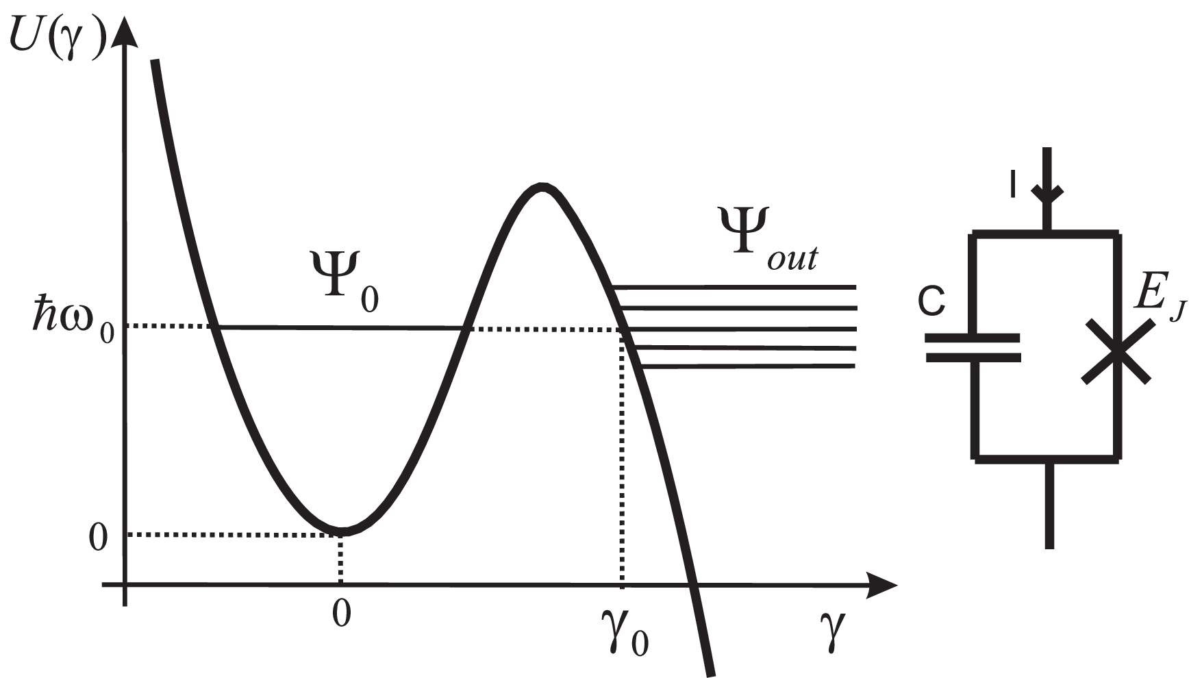
The charge and the magnetic flux (or equivalently the number of Cooper pairs and the relative phase ) are canonically conjugate variables. Hamilton’s equations of motion give
| (2) | |||||
| (3) |
The first equation Eq. (2) is in fact Josephson’s famous formula: a finite voltage across a junction is related to a change in phase. Equation (3) is Kirchhoff’s law for currents. The connection between this equation and Farady’s law can be understood if one considers a superconducting ring interrupted by a Josephson junction. If we can neglect the inductance of the ring itself, then the quantity equals the magnetic flux through the ring: according to Faraday’s law, a change in this flux produces indeed a voltage which equals the voltage across the junction . The second equation Eq. (3) expresses one of Kirchhoff’s laws (conservation of charge in a node of an electrical circuit). The current is the current due to the Josephson effect. This current can be used to define a Josephson nonlinear inductance , and using Eq. (2) we find that
| (4) |
Thus, a Josephson junction can be regarded as an LC-oscillator consisting of a flux-dependent nonlinear inductor in parallel with a capacitor. The inverse of the Josephson inductance measures the curvature of the washboard potential energy at any point - in the same way as the inverse of capacitance is the second derivative of the charging energy .
The quantization of this system follows the usual recipe in quantum mechanics: quantum-mechanical effects become important if the temperature is low enough (lower than the energy level separation), which turns out to be the case for say typical Aluminum or Niobium junctions thermally anchored to the mixing chamber of a dilution refrigerator and with carefully filtered biased lines. The preferred variables to describe a quantized junction are the non-commuting charge and flux operators, (or ). It can be readily checked that the Heisenberg equations of motion are formally identical (all variables being now understood as operators) with the Josephson-Kirchhoff relations Eq. (2) and Eq. (3).
The physics of Josephson pendulums is not unique to metallic junctions: the pendulum Hamiltonian can be used in any situation in which two superfluids are connected by a weak junction. Consider for instance the case of bosonic atoms confined in a two-well potential, a situation which can be realized with alkali atoms trapped in optical lattices.[11] The Hamiltonian of this system is a two-site Bose-Hubbard model with two components: an intrawell interaction energy and a tunneling part,
| (5) |
where the annihilation operators refer to the two wells. In this problem, the total number of particles is a constant of motion. Clearly what happens in this system is that the dynamics can be described as an oscillation of the relative number of particles between the wells. In the regime (sometimes[11] called the Josephson regime of a two-well Bose-Einstein condensate) one can introduce the variables
| (6) |
we find that, up to constant terms, the Hamiltonian Eq. (5) assumes the form of a pendulum (without the bias term),
| (7) |
In the presence of a bias current (or, in the case of alkali atoms, if the optical lattice is tilted in the gravitational field) the washboard potential allows a particle to tunnel in the semi-continuum of energy states immediately outside the well. How do we understand quantum-mechanically this process? Surely, this is an ubiquitous phenomenon which occurs for instance from nuclear -decay to excited atoms emitting photons in vacuum: the physics is governed by the classical exponential law, which states that the fraction of undecayed particles after a time is , where is the decay rate.
3 IRREVERSIBILITY
For a Josephson junction, the decay is essentially a tunneling process between the state localized in one of the wells on one hand (which we call ), and the states outside the well (Fig. 1); the generic form for the macroscopic wavefunction at any time would then be[12]
| (8) |
Here the states are approximately orthogonal to each other and normalized to 1. The decay amplitude , which, when squared, gives the correct classical decay probability law, is not straightforward to understand. Quantum-mechanically, the factor in front of a mode should be an exponential of an imaginary number (a product of energy and time divided by ), much like . Also, the Schrödinger equation is time-reversible, while Eq. (8) is clearly irreversible.
To understand where irreversibility results from, let us consider a simple model[12] in which the state can tunnel into the continuum of states outside the barrier; the Hamiltonian for this model is
| (9) |
and the wavefunction can be expanded as
| (10) |
This problem can be solved[12] using the Laplace transform and the classical decay law results immediately. Here we would like to gain a better intuitive understanding of the mechanism that leads to the appearance of a decay from the otherwise reversible Schrödinger equation. Let us start by considering the Hamiltonian Eq. (9), this time written for a discrete set of out-of-the-well states , with ,
| (11) |
The corresponding wavefunction expansion
| (12) |
results, when used with the Schrödinger equation , in an integrodifferential equation for ,
| (13) |
We now assume that the density of states (let us call it ) and the tunneling amplitude are slowly varying around the frequency , near which the sum in the last part of the expression Eq. (13) above is non-zero. This yields
Inserting this result into Eq. (13) we obtain
| (14) |
where is the decay rate. This set of approximations (sometimes called Weisskopf-Wigner theory[1]) leads to the same formula for the decay rate as given by the Fermi golden rule (first order time-dependent perturbation theory) for transitions between a discrete level and a continuum of states.
Let us now give a numerical illustration for this procedure. We take energy-independent and we solve numerically the Schrödinger equation (with and ; as a result time has no units). We consider 50 states such that (in other words the states are equally spaced around the resonance energy level set by ). Here is the energy separation between the states (the inverse of the density of states). Clearly, keeping the number of states constant and going to lower and lower values of the energy separation , the states tend to merge into a single level, resonant with . In this case, as expected, the particle oscillates between the intrawell state and the level outside the well; in our simulation, we see this as oscillations between 0 and 1 of the probability . For larger values of , the states began to separate and the dynamics is different. In Fig. 2 we present the probability for . The inset shows the approximately exponential decay of the probability to find the system in the initial state . At larger time scales, some peaks appear (corresponding to the particle returning to the well) due to accidental destructive interference of the amplitudes corresponding to the states outside the well. This is a coincidental effect resembling the revival and collapses of the wavefunction in quantum optics; it can be removed either by increasing the number of states of by making the energy separation between them not so uniform. In Fig. 3 we show the results of the second strategy, again with 50 states, , and , but this time with , where is a random fraction between 0 and 1. We notice that the possibility of large accidental constructive interference in the well is reduced, and also that the shape of the decay is very similar to that of the inset of Fig. 2 (we have checked this statement for various other values of ).


We have then demonstrated that the Schödinger equation, albeit reversible, can lead to an irreversible, decay-type evolution when a large number of states is involved. This effect is related to the very small chance of having a constructive interference that would reconstruct the initial wavefunction.
4 THE QUANTUM MEASUREMENT PROBLEM
Let us now consider the measurement problem for a typical superconducting qubit coupled to a read-out system based on switching probabilities. The case of Quantronium[7] is instructive in this sense.

Here, a split Cooper pair box with Josephson energy per junction is coupled to a larger junction of electric capacitance . To maximize the decoherence time, the qubit is kept at the optimal point for which the charging energy of the states and is degenerate ( counts the excess number of Cooper pairs on the island). The qubit states are of the Stern-Gerlach spin-1/2 type, given approximately by and ; in this basis the Hamiltonian is
| (15) |
The macroscopic wavefunction is then spin-dependent
| (16) |
where each component evolves according to
| (17) |
with a spin-dependent wasboard potential . When the bias current is raised adiabatically close to the critical current of the large junction, this leads to two tunneling rates which can be calculated from by standard WKB methods.
We have shown[12] that for a measurement sequence in Quantronium, if we prepare the qubit in the state , then the macroscopic quantum state of the whole system evolves during the measurement sequence as
| (18) | |||||
Here the normalization of is to 1 - not the same as in the previous work[12] where to keep the equations shorter we have normalized to . This equation leads immediately to a formula for the switching probability during an interval ,
| (19) |
Equation (19) above describes precisely the oscillations seen in the experiment, with and dependent on the duration of the microwave pulse (as sine and cosine functions, with Rabi frequency set by the microwave intensity[7]).
What type of measurement does Eq. (18) describe? Let us consider the case of ideal visibility (not yet achieved experimentally), namely the situation in which the states and can be distinguished 100% by the switching or non-switching of the large junction: this means , and . The switching probability therefore simplifies to , and the state Eq. (18) becomes
| (20) |
This is precisely the form of a von Neumann picture of quantum measurement. Initially the qubit is prepared in a superposition of and , and the read-out junction is in the ground state, and during the ”interaction” between the qubit and the junction (due to lowering the potential barrier by increasing the bias current), the two subsystems become entangled. The next step is the collapse of the wavefunction onto one of the components or , with corresponding probabilities and .
One thus immediately sees that Josephson-based superconducting quantum circuits are a perfect tool to study the conceptual foundations of quantum mechanics. A first observation is that the collapse of the wavefunction is a necessary ingredient in the fabric of the quantum formalism, albeit a rather unnatural one from a conceptual point of view. There is no way to get around this postulate by involving more and more subsystems between the qubit and the experimentalist, as it should be clear from the case of Quantronium, where the large junction does precisely the ”interpolation” between the qubit and the classical world. The same argument goes also if one involves the degrees of freedom of (typically) the electromagnetic environment: to obtain the ”real”, classical probabilities, we are simply bound to collapse a more complicated wavefunction. The conceptual problem here is that the choice of states onto which the collapse happens is external to the theory itself. In our case, we know that the experimentalist either sees or does not see a switching event (by the appearance of a relatively large spike in the voltage across the junction, easily measurable by a voltmeter), therefore we know that for example will be correlated with the classical movement of the (macroscopic) voltmeter indicator (pointer). But this is not a consequence of the theory: it is rather an external ingredient. Indeed, quantum theory allows us equally well to do the collapse on a superposition of and . This observation is at the core of the issues associated with the Schrödinger’s cat measurement paradoxes: the punch line of this famous argument is that, if we insist that the quantum-mechanical wavefunction is not just a mathematical instrument to describe the outcomes of a given experiment but is ”real” in the same sense as the waves on a lake are, then we must admit that superpositions of macroscopic objects could exist. The experimental test of this possibility is of great importance for the foundations of quantum theory, and Josephson circuits are now becoming an essential instrument in the toolbox of the future quantum mechanic.
5 CONCLUSIONS
We have investigated the physics of switching in Josephson junctions and we have described how this type of irreversible behavior emerges from the Schrödinger dynamics on a large number of states. For qubit-junction systems, we have analyzed the measurement process and we have shown that it is of von Neumann type. For superconducting circuits, as with all other quantum-mechanical systems, standard quantum theory allows us to describe quantitatively how Schödinger’s cats die, but offer no insight into the problem of how they choose the states onto which to collapse.
ACKNOWLEDGMENTS
This work was supported through a Marie Curie Fellowship (HPMF-CT-2002-01893) and an Acad. Res. Fellowship; it is also part of EU SQUBIT-2 (IST-1999-10673), Academy of Finland TULE No.7205476, CoE in Nuclear and Condensed Matter Physics JyU, and Tekes/FinnNano MOME.
References
- [1] M. O. Scully and M. Suhail Zubairy, Quantum Optics (Cambridge University Press, Cambridge 1997).
- [2] Y. Makhlin, G. Schn, and A. Shnirman, Nature 386, 305 (1999); J. E. Mooij et. al., Science 285, 1036 (1999); Yu. Makhlin, G. Schn, and A. Shnirman, Rev. Mod. Phys. 73, 357 (2001).
- [3] Y. Nakamura, Y. A. Pashkin, and J. S. Tsai, Nature, 398, 786 (1999); C. H. van der Wal et. al., Science 290, 773 (2000); J. R. Friedman et. al., Nature 406, 43 (2000).
- [4] Yu. A. Paskin et. al., Nature 421, 823 (2003); T. Yamamoto et. al., Nature 425, 941 (2003); T. Duty, D. Gunnarsson, K. Bladh, and P. Delsing, Phys. Rev. B 69, 140503(R) (2004).
- [5] J. M. Martinis, S. Nam, J. Aumentado, and C. Urbina, Phys. Rev. Lett. 89, 117901 (2002); J. Claudon, F. Balestro, F. W. J. Hekking, and O. Buisson, Phys. Rev. Lett. 93, 187003 (2004).
- [6] I. Chiorescu, Y. Nakamura, C. J. P. M. Harmans, and J. E. Mooij, Science 299, 1869 (2003).
- [7] D. Vion at. al, Science 296, 886 (2002); A. Cottet et. al., Physica C 367, 197 (2002); D. Vion et. al. Phys. Scr. T 102, 162 (2002); A. Cottet, Ph. D. thesis, Univ. Paris VI (2002); E. Collin et. al., Phys. Rev. Lett. 93, 157005 (2004); G. Ithier, et. al. Phys. Rev. B 72, 134519 (2005).
- [8] J. Clarke, A. N. Cleland, M. H. Devoret, D. Esteve, and J. M. Martinis, Science 239, 992 (1988).
- [9] A. J. Leggett, Suppl. Progr. Theor. Phys. 69, 80 (1980).
- [10] M. Tinkham, Introduction to Superconductivity, 2nd ed. (McGraw-Hill Inc., New York, 1996); A. Barone and G. Paternò, Physics and Applications of the Josephson Effect (Wiley, New York, 1982).
- [11] A J. Leggett, Rev. Mod. Phys. 73, 307 (2001), G. S. Paraoanu, S. Kohler, F. Sols, and A. J. Leggett, J. Phys. B 34, 4689 (2001); G. S. Paraoanu, M. Rodriguez, and P. Törmä , Phys. Rev. A 66, R041603 (2002); G. S. Paraoanu, Phys. Rev. A 67, 023607 (2003).
- [12] G. S. Paraoanu, Phys. Rev. B 72, 134528 (2005).