Estimation of conditional laws given an extreme component

Anne-Laure Fougères ^†^†thanks: Université Claude Bernard - Lyon 1 Philippe Soulier ^†^†thanks: Université Paris Ouest-Nanterre

Abstract

Let $(X,Y)$ be a bivariate random vector. The estimation of a probability of the form $P(Y\leq y\mid X>t)$ is challenging when $t$ is large, and a fruitful approach consists in studying, if it exists, the limiting conditional distribution of the random vector $(X,Y)$ , suitably normalized, given that $X$ is large. There already exists a wide literature on bivariate models for which this limiting distribution exists. In this paper, a statistical analysis of this problem is done. Estimators of the limiting distribution (which is assumed to exist) and the normalizing functions are provided, as well as an estimator of the conditional quantile function when the conditioning event is extreme. Consistency of the estimators is proved and a functional central limit theorem for the estimator of the limiting distribution is obtained. The small sample behavior of the estimator of the conditional quantile function is illustrated through simulations. Some real data are analysed.

1 Introduction

Let $(X,Y)$ be a bivariate random vector for which the conditional distribution of $Y$ given that $X>t$ is of interest, for values of $t$ such that the conditioning event is a rare event. This happens for example when the possible contagion between two dependent market returns $X$ and $Y$ is investigated, see e.g. Bradley and Taqqu (2004) or Abdous et al. (2008). The estimation of a probability of the form $P(Y\leq y\mid X>t)$ starts to be challenging as soon as $t$ is large, since the conditional empirical distribution becomes useless when no observations are available. A fruitful alternative approach consists in studying, if it exists, the limiting distribution of the random vector $(X,Y)$ conditionally on $X$ being large. This corresponds to assuming that there exist functions $m$ , $a$ and $\psi$ , and a bivariate distribution function (cdf) $F$ on $[0,\infty)\times(-\infty,\infty)$ with non degenerate marginal distributions, such that

\displaystyle\lim_{t\to\infty}\mathbb{P}(X\leq t+\psi(t)x\;;\;Y\leq m(t)+a(t)y\mid X>t)=F(x,y)

(1)

at all points of continuity of $F$ . This assumption has been called a “conditional extreme value” (CEV) model by Das and Resnick (2009). Some of its main consequences were thoroughly investigated by Heffernan and Resnick (2007) and its relationship to standard bivariate extreme value theory has been investigated in Das and Resnick (2010). In particular, Condition (1) does not imply that the distribution of $(X,Y)$ belongs to the domain of attraction of a bivariate extreme value distribution. Examples of random vectors which are not in the domain of attraction of a bivariate extreme value distribution and still satisfy Condition (1) are given in Das and Resnick (2010) and Fougères and Soulier (2010) (see Section 3.1 therein for a related discussion).

The classical bivariate extreme value condition means that there exist normalizing functions $c_{1},c_{2}$ , $d_{1},d_{2}$ and a bivariate extreme value distribution $H$ such that

\displaystyle\lim_{n\to\infty}\mathbb{P}^{n}(X\leq c_{1}(n)+d_{1}(n)x\;,Y\leq c_{2}(n)+d_{2}(n)y)=H(x,y)\;.

(2)

The function $c_{1}$ can always be chosen such that $\lim_{s\to\infty}s\mathbb{P}(X>c_{1}(s))=1$ , and then it is easily seen that

\displaystyle\lim_{s\to\infty}\mathbb{P}(X\leq c_{1}(s)+d_{1}(s)x\,,\,Y\leq c_{2}(s)+d_{2}(s)y\mid X>c_{1}(s))=-\log H(0,y)+\log H(x,y)\;.

Two cases are possible: either the limiting distribution $H$ is in product form or it is not in product form. In extreme value theory, the former case is referred to as asymptotic independence, and the latter is referred to as asymptotic dependence. In the case of asymptotic dependence, then $F(x,y)=-\log H(0,y)+\log H(x,y)$ is a non degenerate distribution function, and the CEV condition (1) holds. Thus the problem is entirely solved by the standard extreme value theory in the case of asymptotic dependence. In the case of asymptotic independence, i.e. $H(x,y)=H_{1}(x)H_{2}(y)$ , then $-\log H(0,y)+\log H(x,y)=-\log H_{1}(x)$ , so that the limit is degenerate with respect to $y$ . In the case of asymptotic independence, standard bivariate extreme value theory is useless to check the CEV condition (1). To summarize this discussion, it appears that the CEV model (1) is potentially useful when the standard bivariate extreme value condition (2) does not hold or when condition (2) holds with asymptotic independence.

It must be noted that the CEV condition (1) always holds when $X,Y$ are independent, $Y$ is non-degenerate and $X$ is in the domain of attraction of a univariate extreme value distribution. This implies that all bivariate distributions $F$ that can be expressed as $F(x,y)=F_{1}(x)F_{2}(y)$ , where $F_{1}$ is a univariate extreme value distribution and $F_{2}$ is any non-degenerate distribution function can appear as a limiting distribution in (1). This trivial consideration has the consequence that it is very difficult to have a general theory for the conditional extreme value model and to define statistical procedures valid in all cases. Rather, it is necessary to study classes of bivariate distributions that satisfy the CEV condition (1) and to establish statistical procedures suited to these classes.

Models for which condition (1) holds have already been investigated in many references. Eddy and Gale (1981) and Berman (1982); Berman (1992) proved that (1) holds for spherical distributions; bivariate elliptical distributions were investigated by Berman (1982), multivariate elliptical distributions and related distributions by Hashorva (2006); Hashorva (2007) Hashorva et al. (2007). The analysis of the underlying geometric structure (ellipticity of the level sets of the densities) has lead to various generalizations by Barbe (2003) and Balkema and Embrechts (2007). See also Fougères and Soulier (2010) for a recent review on the subject. An important finding of these works is that when the CEV condition is a consequence of such geometric properties, the domain of attraction of the conditioning variable determines the nature of the limiting distribution $F$ in (1). For instance, for the usual bivariate elliptical distributions, if the conditioning variable has a regularly varying right tail, then the limiting distribution $F$ is not in product form, whereas it is in product form if the conditioning variable is in the domain of attraction of the Gumbel law. Other types of models that satisfy Assumption (1) have been studied in Alink et al. (2004), Hashorva (2008); Hashorva (2009a); Hashorva (2009b).

The aim of this paper is the statistical estimation of the functions $a$ and $m$ that appear in (1), as well as the limiting distribution function $F$ . Two problems are considered. The first one is the nonparametric estimation of the limiting distribution and of the normalizing functions. This is done in Section 3 in full generality. We only assume that the CEV condition (1) holds and some additional moment conditions which are necessary to obtain consistency of the estimators. In order to obtain central limit theorems, we also need to assume some kind of second order conditions.

As discussed above, it seems impossible to go beyond these results without making some restrictive assumptions. From Section 4 onwards, we assume that the conditioning variable is in the maximum domain of attraction of the Gumbel law, and that the limiting joint distribution $F$ has product form. This choice leaves out many interesting cases, but is motivated by previous works and has not been considered yet in a statistical study. Under these assumptions, we validate a Kolmogorov-Smirnov type test for the limiting distribution of the $Y$ variable, e.g. the standard Gaussian distribution which appears in many examples. Since we are also interested in the case where the conditioning event is beyond the range of observations, a semiparametric procedure is defined to allow this extrapolation. This again necessitates restrictive assumptions. Those we make are satisfied by several models already investigated (cf. Fougères and Soulier (2010)). Let us finally note that to the best of our knowledge, the estimators of the quantities related to the conditional laws presented in this paper have not been considered before.

The paper is organized as follows. In Section 2, we rephrase (1) in terms of vague convergence of measures in order to use the point process techniques and the results of Heffernan and Resnick (2007). We also introduce moment assumptions which are needed to prove the consistency of the nonparametric estimators introduced in Section 3. A functional central limit theorem for the estimator of the limiting distribution is obtained under a second order condition. In Section 4, a specific analysis of the case of a limiting distribution with product form and $X$ in the domain of attraction of the Gumbel law is done. The functional central limit theorem is used to derive a goodness of fit test for the second marginal of the limiting distribution $F$ . In Section 4.2, semiparametric estimators that allow extrapolations beyond the range of the observations are studied and applied to the estimation of conditional quantiles when the conditioning event is extreme. A simulation study is given in Section 5 to illustrate the small sample behavior of our estimators, of the goodness of fit test proposed in Section 4.1 and of the estimator of the conditional quantile proposed in Section 4.2. These results are applied in Section 6 to some financial data. Section 7 collects the proofs.

2 Assumptions and preliminary results

We first rephrase the convergence (1) in terms of vague convergence of measures, in order to use point process techniques and the results of Heffernan and Resnick (2007). See also Das and Resnick (2009); Das and Resnick (2010). Condition (1) implies that the marginal distribution of $X$ belongs to the domain of attraction of an extreme value distribution with index $\gamma\in\mathbb{R}$ , i.e. there exist normalizing sequences $\{b_{n}\}$ and $\{c_{n}\}$ with $c_{n}>0$ such that $\mathbb{P}(\max_{1\leq i\leq n}(X_{i}-b_{n})/c_{n}\leq x)$ converges to $\exp\{-\bar{P}_{\gamma}(x)\}$ for each $x$ such that $1+\gamma x>0$ , where $\bar{P}_{\gamma}(x)=(1+\gamma x)^{-1/\gamma}$ if $\gamma\neq 0$ and $\bar{P}_{0}(x)=\mathrm{e}^{-x}$ , and the random variables $X_{i}$ are independent copies of $X$ . For simplicity, we assume that $\gamma\geq 0$ , and in the case $\gamma=0$ we assume that the right endpoint of the marginal distribution of $X$ is infinite.

Recall that a measure defined on the Borel sigma-field of a locally compact separable space $E$ is called a Radon measure if it is finite on compact sets. A sequence of Radon measures $\sigma_{n}$ defined on $E$ converges vaguely to a Radon measure $\sigma$ if $\int_{E}f(x)\sigma_{n}(\mathrm{d}x)$ converges to $\int_{E}f(x)\sigma(\mathrm{d}x)$ for all compactly supported function $f$ . See Resnick (1987, Chapter 3) or Heffernan and Resnick (2007, Appendix A3). We will consider vague convergence of Radon measures defined on the Borel sigma-fields of $(-1/\gamma,\infty]$ or $(-1/\gamma,\infty]\times[-\infty,\infty]$ .

Assumption 1.

There exist $\gamma\geq 0$ , monotone functions $a$ , $b$ , $m$ and $\psi$ such that the marginal distribution of $X$ is in the domain of attraction of the extreme value distribution with extreme value index $\gamma$ and the sequence of measures $\nu_{n}$ defined by

\displaystyle\nu_{n}(\cdot)=n\mathbb{P}\left(\left\{\frac{X-b(n)}{\psi\circ b(n)},\frac{Y-m\circ b(n)}{a\circ b(n)}\right\}\in\cdot\right)

converges vaguely on $(-1/\gamma,\infty]\times[-\infty,\infty]$ to a Radon measure $\nu$ such that $\nu([0,\infty)\times(-\infty,\infty))=1$ , the distribution function $y\mapsto\nu([0,\infty)\times(-\infty,y])$ is non degenerate and the application $(x,y)\mapsto\nu([x,\infty)\times(-\infty,y])$ is continuous on $(-1/\gamma,\infty]\times[-\infty,\infty]$ .

Assumption 1 is equivalent to assumptions 1.2 and 1.3 of Das and Resnick (2009) and to Assumption (5) of Heffernan and Resnick (2007), apart from the continuity assumption which is needed for statistical purposes such as the Kolmogorov-Smirnov test proposed in Section 4.1. The link between Assumption 1 and Equation (1) is that the limiting distribution $F$ is given, for all positive $x$ and real $y$ , by

\displaystyle F(x,y)=\nu([0,x]\times(-\infty,y])\;.

Assumption 1 also implies that $F$ is continuous and that the sequence of probability distribution functions $F_{n}$ defined, for all positive $x$ and real $y$ , by

\displaystyle F_{n}(x,y)=\nu_{n}([0,x]\times(-\infty,y])

converges to $F$ locally uniformly. Assumption 1 can also be interpreted as the weak convergence to $F$ of the vector $(X-b(n))/\psi\circ b(n),(Y-m\circ b(n))/a\circ b(n))$ conditionally on $X>b(n)$ , i.e. for all bounded continuous function $h$ on $[0,\infty)\times(-\infty,\infty)$ ,

\displaystyle\lim_{n\to\infty}\mathbb{E}\left[h\left(\frac{X-b(n)}{\psi\circ b(n)},\frac{Y-m\circ b(n)}{a\circ b(n)}\right)\mid X>b(n)\right]=\int_{0}^{\infty}\int_{-\infty}^{\infty}h(x,y)F(\mathrm{d}x,\mathrm{d}y)\;.

(3)

Remark 1.

All results concerning only the marginal distribution of $X$ are obtained by applying the usual extreme value theory. In particular, the functions $\psi$ and $b$ are determined by the marginal distribution of $X$ only. The function $b$ can and will be chosen as $b=(1/(1-F_{X}))^{\leftarrow}$ where $F_{X}$ is the distribution function of $X$ . The function $\psi$ satisfies

\displaystyle\lim_{x\to+\infty}\frac{\psi(x+\psi(x)u)}{\psi(x)}=1+\gamma u\;.

(4)

See (Resnick, 1987, Propositions 1.4 and 1.11). For any $x>-1/\gamma$ , it holds that

\displaystyle\nu([x,\infty]\times[-\infty,\infty])=(1+\gamma x)^{-1/\gamma}\;,

with the usual convention that this expression must be read as $\mathrm{e}^{-x}$ when $\gamma=0$ .

Remark 2.

Assumption 1 has little implications on the functions $a$ and $m$ and on the distribution $\Psi$ defined by

\displaystyle\Psi(z)=\int_{0}^{\infty}\int_{-\infty}^{z}\nu(\mathrm{d}x,\mathrm{d}y)\;.

If $Y$ is independent of $X$ , then $\Psi$ is the distribution of $Y$ , $a\equiv 1$ and $m\equiv 0$ . Thus $\Psi$ can be any probability distribution and it is not necessarily an extreme value distribution.

Remark 3.

If the pair $(X,Y)$ satisfies Assumption 1, then so does any affine coordinatewise transformation of $(X,Y)$ . For instance, if $X$ and $Y$ have finite mean and variance, then $((X-\mathbb{E}[X])/\mathrm{var}^{1/2}(X),(Y-\mathbb{E}[Y])/\mathrm{var}^{1/2}(Y))$ also satisfies Assumption 1. But non linear transformations of $(X,Y)$ do not necessarily satisfy the assumption. Even though the conditioning variable can be standardized, the simultaneous transformation of $X$ and $Y$ to random variables with prescribed marginal distributions is not always possible. This problem has been thoroughly investigated in (Heffernan and Resnick, 2007, Section 7). It is never possible in the cases where the joint limiting distribution is a product measure. Consequently, we do not make any specific assumption on the marginal distributions of $X$ and $Y$ .

Obviously, the functions $a$ and $m$ are defined up to asymptotic equivalence, i.e. if $m^{\prime}$ and $a^{\prime}$ satisfy

\displaystyle\lim_{x\to\infty}\frac{a^{\prime}(x)}{a(x)}=1\;,\ \ \lim_{x\to\infty}\frac{m(x)-m^{\prime}(x)}{a(x)}=0\;,

then the measure $\nu^{\prime}_{n}$ defined as $\nu_{n}$ but with $a^{\prime}$ and $m^{\prime}$ instead of $a$ and $m$ converges vaguely to the same limit measure $\nu$ . Beyond this trivial remark, the following result summarizes Heffernan and Resnick (2007, Propositions 1 and 2) and contains most of what can be infered from Assumption 1. Recall that a function $f$ defined on a neighborhood of infinity is said to be regularly varying if there exists a constant $\alpha\in\mathbb{R}$ such that

\displaystyle\lim_{x\to\infty}\frac{f(tx)}{f(x)}=t^{\alpha}

for all $t>0$ . If $\alpha=0$ , the function is called slowly varying.

Lemma 1.

Under Assumption 1, there exists $\zeta\in{\mathbb{R}}$ such that the function $a\circ b$ is regularly varying at infinity with index $\zeta$ and the function $m$ satisfies

\displaystyle\lim_{t\to\infty}\frac{m\circ b(tx)-m\circ b(t)}{a\circ b(t)}=J_{\zeta}(x)\;,

with $J_{\zeta}(x)=(x^{\zeta}-1)/\zeta$ if $\zeta\neq 0$ and $J_{0}(x)=c\log(x)$ for some $c\in{\mathbb{R}}$ , and the convergence is locally uniform on $(0,\infty)$ .

For a sequence $(X_{i},Y_{i})$ , $1\leq i\leq n$ , let $X_{(n:i)}$ denote the $i$ -th order statistic and $Y_{[n:i]}$ denote its concomitant, i.e. $X_{(n:1)}$ ,…, $X_{(n:n)}$ is the ordering of $X_{1},\dots,X_{n}$ in increasing order, and $Y_{[n:i]}$ is the $Y$ -variable corresponding to $X_{(n:i)}$ .

Recall that an intermediate sequence is a sequence of integers $k_{n}$ such that $\lim_{n\to\infty}k_{n}=\lim_{n\to\infty}n/k_{n}=\infty$ . In accordance with common use and for the clarity of notation, the dependence on $n$ will be implicit in the sequel.

Define the random measure

\displaystyle\tilde{\nu}_{n}=\frac{1}{k}\sum_{i=1}^{n}\delta_{(\{X_{i}-b(n/k)\}/\psi\circ b(n/k),\{Y_{i}-m\circ b(n/k)\}/a\circ b(n/k))}\;.

(5)

Applying Resnick (1986, Proposition 5.3) (see also Resnick (1987, Exercise 3.5.7)), we straightforwardly obtain the following result.

Proposition 2.

If Assumption 1 holds, then for any intermediate sequence $k$ , $\tilde{\nu}_{n}$ converges weakly to $\nu$ locally uniformly on $(-1/\gamma,\infty]\times[-\infty,\infty]$ .

Consequently, $\tilde{\nu}_{n}([0,x]\times(-\infty,y])$ converges weakly locally uniformly to $F(x,y)$ . But $\tilde{\nu}_{n}$ is not an estimator, since its definition involves the unknown functions $a$ and $m$ . In order to define estimators of these functions, and of the distribution function $F$ , we will need to prove convergence of integrals of unbounded functions with respect to the random measure $\tilde{\nu}_{n}$ . Therefore we need to strengthen Assumption 1.

Assumption 2.

There exists $p^{*}>0$ , $q^{*}>0$ such that for any $\epsilon\in(0,1/\gamma)$ ,

\displaystyle\lim_{n\to\infty}\int_{-\epsilon}^{\infty}\int_{-\infty}^{\infty}|x|^{p^{*}}|y|^{q^{*}}\nu_{n}(\mathrm{d}x,\mathrm{d}y)=\int_{-\epsilon}^{\infty}\int_{-\infty}^{\infty}|x|^{p^{*}}|y|^{q^{*}}\nu(\mathrm{d}x,\mathrm{d}y)\;.

(6)

Condition (6) can be seen as a strengthening of (1) and (3) in order to obtain the convergence of conditional moments. Under Assumption 2, for all $0<p\leq p^{*}$ and $0<q\leq q^{*}$ , it holds that

\displaystyle\lim_{t\to\infty}\frac{\mathbb{E}[(X-t)^{p}|Y-m(t)|^{q}\mid X>t]}{\psi^{p}(t)a^{q}(t)}=\int_{0}^{\infty}\int_{-\infty}^{\infty}x^{p}|y|^{q}\nu(\mathrm{d}x,\mathrm{d}y)\;.

(7)

For the reason mentioned in Remark 1, Assumption 1 implies the convergence (6) with $q^{*}=0$ and any $p^{*}<1/\gamma$ . Conversely, Assumption 2 implies $\gamma<1/p^{*}$ . In applications, it will be assumed that $q^{*}\geq 2$ . The function $a$ and the limiting measure $\nu$ are defined up to a change of scale, thus, without loss of generality, we assume henceforth that

\displaystyle\int_{0}^{\infty}\int_{-\infty}^{\infty}y^{2}\,\nu(\mathrm{d}x,\mathrm{d}y)=\int_{-\infty}^{\infty}y^{2}\Psi(\mathrm{d}y)=1\;.

(8)

Proposition 3.

If Assumptions 1 and 2 hold, then for any intermediate sequence $k$ and any continuous function $g$ such that $|g(x,y)|\leq C(|x|\vee 1)^{p^{*}}(|y|\vee 1)^{q^{*}}$ , for any $\epsilon\in(0,1/\gamma)$ ,

\displaystyle\int_{-\epsilon}^{\infty}\int_{-\infty}^{\infty}g(x,y)\tilde{\nu}_{n}(\mathrm{d}x,\mathrm{d}y)\to_{P}\int_{-\epsilon}^{\infty}\int_{-\infty}^{\infty}g(x,y)\nu(\mathrm{d}x,\mathrm{d}y)\;.

(9)

For historical interest, we can also mention the following consequence of Assumption 1. This result was obtained by Eddy and Gale (1981, Theorem 6.1) under the restrictive additional assumption of a spherical distribution. Related results can also be found in Hashorva (2007); Hashorva (2008) and Nagaraja and David (1994).

Proposition 4.

Under Assumption 1, $(\{X_{(n:n)}-b(n)\}/\psi\circ b(n),\{Y_{[n:n]}-m\circ b(n)\}/a\circ b(n))$ converges weakly to $F$ .

Since $\Psi$ is the second marginal of $F$ , this result implies that $\{Y_{[n:n]}-m\circ b(n)\}/a\circ b(n)$ converges weakly to $\Psi$ . If $F$ is a product measure, (or equivalently if $\nu$ is a product measure), then $\{Y_{[n:n]}-m\circ b(n)\}/a\circ b(n)$ is asymptotically independent of $\{X_{(n:n)}-b(n)\}/\psi\circ b(n)$ in the usual sense that the limiting distribution is a product measure.

Let us finally mention that Davydov and Egorov (2000) obtained functional limit theorems for sums of concomitants corresponding to a number $k$ of order statistics such that $k/n\nrightarrow 0$ . Therefore their problem differs from ours. Their assumptions on the joint distribution of the random pairs are much weaker than Assumption 1, but their results are of a very different nature and it does not seem possible to use them to derive Propositions 2-3 for instance.

3 Nonparametric estimation of $\psi$ , $a$ , $m$ and $F$

In this section, we introduce nonparametric estimators of the functions $\psi$ , $m$ , $a$ and $F$ based on i.i.d. observations $(X_{1},Y_{1}),\dots,(X_{n},Y_{n})$ of a bivariate distribution which satisfies Assumption 2.

3.1 Definitions and consistency

In order to estimate nonparametrically the limiting distribution $F$ , we first need nonparametric estimators of the quantities $\psi(X_{(n:n-k)})$ , $m(X_{(n:n-k)})$ and $a(X_{(n:n-k)})$ , with $k$ an intermediate sequence, i.e. such that $k\to\infty$ and $k/n\to 0$ . The estimation of $\psi(X_{(n:n-k)})$ is a well known estimation issue, see e.g. De Haan and Ferreira (2006, Section 4.2). If the extreme value index $\gamma$ of $X$ is less than 1, then $\psi$ can be estimated as the mean residual life. Let $\hat{\gamma}$ be a consistent estimator of $\gamma$ (see e.g. De Haan and Ferreira (2006, Chapter 3) or Beirlant et al. (2004, Chapter 5)) and define

\displaystyle\hat{\psi}(X_{(n:n-k)})=\frac{1-\hat{\gamma}}{k}\sum_{i=1}^{k}\{X_{(n:n-i+1)}-X_{(n:n-k)}\}\;.

(10)

It follows straightforwardly from Proposition 3 that $\hat{\psi}(X_{(n:n-k)})/\psi\circ b(n/k)\to_{P}1$ . If it is moreover assumed (as in Section 4 below) that $\gamma=0$ , then the above estimator can be modified accordingly:

\displaystyle\hat{\psi}(X_{(n:n-k)})=\frac{1}{k}\sum_{i=1}^{k}\{X_{(n:n-i+1)}-X_{(n:n-k)}\}\;.

(11)

In order to estimate $m$ , define

\displaystyle\hat{m}(X_{(n:n-k)})=\frac{\sum_{i=1}^{k}Y_{[n:n-i+1]}\{X_{(n:n-i+1)}-X_{(n:n-k)}\}}{\sum_{i=1}^{k}\{X_{(n:n-i+1)}-X_{(n:n-k)}\}}\;.

(12)

Proposition 5.

If Assumptions 1 and 2 hold with $p^{*}\geq 1$ and $q^{*}\geq 1$ , then, for any intermediate sequence $k$ , it holds that

\displaystyle\frac{\hat{m}(X_{(n:n-k)})-m\circ b(n/k)}{a\circ b(n/k)}\to_{P}\mu\;,

where $\mu=(1-\gamma)\int_{0}^{\infty}\int_{-\infty}^{\infty}xy\nu(\mathrm{d}x,\mathrm{d}y)$ . If moreover $m(x)=\rho x$ and either $\mu=0$ and $a(x)=O(x)$ or $a(x)=o(x)$ then $\hat{m}(X_{(n:n-k)})/X_{(n:n-k)}$ is a consistent estimator of $\rho$ .

Remark 4.

A sufficient condition for $\mu=0$ is the symmetry of the measure $\nu$ with respect to the second variable. This happens e.g. when if $\nu$ is a product measure and the distribution $\Psi$ is symmetric.

Remark 5.

As explained above, the assumption $p^{\star}\geq 1$ in Proposition 5 implies that $\gamma<1$ . If $\gamma\geq 1$ , which implies that $|X|$ has an infinite mean, the previous estimators of $\psi$ and $m$ need not be consistent. Consistent estimators of $\gamma$ and $\psi$ can be found in (De Haan and Ferreira, 2006, Section 4.2) but it is not clear how to define a consistent estimator of $m$ in this context.

We now estimate $a(X_{(n:n-k)})$ . Many estimators can be defined, each needing an ad hoc moment assumption. The one we have chosen needs $q^{*}\geq 2$ in Assumption 2. Define

\displaystyle\hat{a}(X_{(n:n-k)})=\left\{\frac{1}{k}\sum_{i=1}^{k}\{Y_{[n:n-i+1]}-\hat{m}(X_{(n:n-k)})\}^{2}\right\}^{1/2}\;.

(13)

Proposition 6.

If Assumptions 1 and Assumption 2 hold with $p^{*}\geq 1$ and $q^{*}\geq 2$ , and if $\mu=0$ , then, for any intermediate sequence $k$ , it holds that

\displaystyle\hat{a}(X_{(n:n-k)})/a\circ b(n/k)\to_{P}1\;.

Remark 6.

Under Assumption 1 with $q^{*}\geq 2$ , the first moment of $\Psi$ is finite and if $\mu\neq 0$ , then $\hat{a}(X_{(n:n-k)})/a\circ b(n/k)\to_{P}\tau$ , with

\displaystyle\tau^{2}=1-2\mu\int_{-\infty}^{\infty}y\Psi(\mathrm{d}y)+\mu^{2}\;.

(14)

We can now consider the nonparametric estimator of the limiting joint distribution $F$ . Define

\hat{F}(x,y)\\ =\frac{1}{k}\sum_{i=1}^{k}\mathbf{1}_{\{X_{(n:n-i+1)}\leq X_{(n:n-k)}+\hat{\psi}(X_{(n:n-k)})x\}}\times\mathbf{1}_{\{Y_{[n:n-i+1]}\leq\hat{m}(X_{(n:n-k)})+\hat{a}(X_{(n:n-k)})y\}}\;.

(15)

Denote $u_{n}={\hat{\psi}(X_{(n:n-k)})}/{\psi\circ b(n/k)}$ and

\displaystyle\tilde{x}_{n}=\frac{X_{(n:n-k)}-b(n/k)}{\psi\circ b(n/k)}\;,\ \ v_{n}=\frac{\hat{a}(X_{(n:n-k)})}{a\circ b(n/k)}\;,\ \ \ \xi_{n}=\frac{\hat{m}(X_{(n:n-k)})-m\circ b(n/k)}{a\circ b(n/k)}\;.

(16)

Then

\displaystyle\hat{F}(x,y)=\tilde{\nu}_{n}([\tilde{x}_{n},\tilde{x}_{n}+u_{n}x]\times(-\infty,\xi_{n}+v_{n}y])\;.

Thus Propositions 2, 5 and 6 easily yield the consistency of $\hat{F}(x,y)$ , as stated in the following theorem.

Theorem 7.

Under Assumptions 1 and 2 with $p^{*}\geq 1$ and $q^{*}\geq 2$ , if $\mu=0$ , then for any intermediate sequence $k$ , $\hat{F}(x,y)$ converges weakly to $F(x,y)$ .

We can also define an estimator of the second marginal $\Psi$ of $F$ . Denote

\displaystyle\hat{\Psi}(y)

\displaystyle=\frac{1}{k}\sum_{i=1}^{k}\mathbf{1}_{\{Y_{[n:n-i+1]}\leq\hat{m}(X_{(n:n-k)})+\hat{a}(X_{(n:n-k)})y\}}\;.

(17)

Then, under the assumptions of Theorem 7, $\hat{\Psi}$ also converges to $\Psi$ . Note that if $\mu\neq 0$ , then $\hat{\Psi}(z)$ converges weakly to $\Psi(\mu+\tau z)$ , with $\tau$ defined in (14).

3.2 Central limit theorems

In order to obtain central limit theorems, we need to strengthen Assumptions 1 and 2.

Assumption 3.

There exist positive real numbers $p^{\dagger}$ and $q^{\dagger}$ , a function $c$ such that $\lim_{t\to\infty}c(t)=0$ and a Radon measure $\mu^{\dagger}$ on $(-1/\gamma,\infty)\times(-\infty,\infty)$ such that for any $\epsilon\in(0,1/\gamma)$ , and any measurable function $h$ such that $|h(x,y)|\leq(|x|\vee 1)^{p^{\dagger}}(|y|\vee 1)^{q^{\dagger}}$ , it holds that

\displaystyle\int_{-\epsilon}^{\infty}\int_{-\infty}^{\infty}|h(x,y)|\mu^{\dagger}(\mathrm{d}x,\mathrm{d}y)<\infty\;,

and

\left|\int_{-\epsilon}^{\infty}\int_{-\infty}^{\infty}h(x,y)\nu_{n}(\mathrm{d}x,\mathrm{d}y)-\int_{-\epsilon}^{\infty}\int_{-\infty}^{\infty}h(x,y)\nu(\mathrm{d}x,\mathrm{d}y)\right|\\ \leq c\circ b(n)\int_{-\epsilon}^{\infty}\int_{-\infty}^{\infty}|h(x,y)|\mu^{\dagger}(\mathrm{d}x,\mathrm{d}y)\;.

(18)

Remark 7.

Taking $h=\mathbf{1}_{[0,x]\times(-\infty,y]}$ , (18) yields

\displaystyle|F_{n}(x,y)-F(x,y)|\leq c\circ b(n)\mu^{\dagger}([0,x]\times(-\infty,y])

(19)

where $F_{n}(x,y)=\nu_{n}([0,x]\times(-\infty,y])$ . This is a classical second order condition (see e.g. de Haan and Resnick (1993, Condition 4.1)), which gives a non uniform rate of convergence in Condition (1). The condition (18) is stronger than (19) in the sense that it moreover gives a rate of convergence for conditional moments. Since Assumption 3 implies that the first marginal of $F$ has finite moments up to the order $p^{\dagger}$ , it also implies that $\gamma<1/p^{\dagger}$ .

For a sequence $k$ depending on $n$ , define the random measure $\tilde{\mu}_{n}$ by

\displaystyle\tilde{\mu}_{n}=k^{1/2}\left(\tilde{\nu}_{n}-\nu\right)\;

and denote

\displaystyle W_{n}(x,y)=\tilde{\mu}_{n}((x,\infty)\times(-\infty,y]).

The next result states the functional convergence of $W_{n}$ in the space $\mathcal{D}((-1/\gamma,\infty)\times(-\infty,\infty))$ of right-continuous and left-limited functions, endowed with Skorohod’s $J_{1}$ topology.

Proposition 8.

If Assumption 3 holds with $p^{\dagger}\geq 2$ and $q^{\dagger}\geq 4$ and if the sequence $k$ is chosen such that

\displaystyle\lim_{n\to\infty}k^{1/2}c\circ b(n/k)=0\;,

(20)

then $k$ is an intermediate sequence and the sequence of processes $W_{n}$ converges weakly in $\mathcal{D}((-1/\gamma,\infty)\times(-\infty,\infty))$ to a Gaussian process $W$ with covariance function

\displaystyle\mathrm{cov}(W(x,y),W(x^{\prime},y^{\prime}))=\nu([x\vee x^{\prime},+\infty]\times[-\infty,y\wedge y^{\prime}])\;.

(21)

Moreover, the sequence of random measures $\tilde{\mu}_{n}$ converges weakly (in the sense of finite dimensional distributions) to an independently scattered Gaussian random measure $W$ with control measure $\nu$ on the space of measurable functions $g$ such that $|g(x,y)|^{2}\leq C(x\vee 1)^{p^{\dagger}}(|y|\vee 1)^{q^{\dagger}}$ , i.e. $W(g)$ is a centered Gaussian random variable with variance

\displaystyle\int_{-1/\gamma}^{\infty}\int_{-\infty}^{\infty}g^{2}(s,t)\,\nu(\mathrm{d}s,\mathrm{d}t)

and $W(g)$ , $W(h)$ are independent if $\int gh\,\mathrm{d}\nu=0$ .

The proof is in section 7. Applying Proposition 8, we easily obtain the following corollary. For $i,j\geq 0$ , denote $g_{i,j}(x,y)=x^{i}y^{j}\mathbf{1}_{\{x>0\}}$ .

Corollary 9.

Under the assumptions of Proposition 8 and if moreover $\mu=0$ , then

\displaystyle k^{1/2}\left\{\frac{X_{(n:n-k)}-b(n/k)}{\psi\circ b(n/k)}\;,\frac{\hat{m}(X_{(n:n-k)})-m\circ b(n/k)}{a\circ b(n/k)}\;,\frac{\hat{a}(X_{(n:n-k)})}{a\circ b(n/k)}-1\right\}

converges jointly with $k^{1/2}(\tilde{\nu}_{n}-\nu)$ to a Gaussian vector which can be expressed as

(W(g_{0,0}),(1-\gamma)W(g_{1,1}),\frac{1}{2}W(g_{0,2}))\;.

Proposition 8 and Corollary 9 straightforwardly yield a functional central limit theorem for the estimator $\hat{\Psi}$ of $\Psi$ defined in (17). Recall that $F(x,y)=\nu([0,x]\times(-\infty,y])$ .

Theorem 10.

If Assumption 3 holds with $p^{\dagger}\geq 2$ and $q^{\dagger}\geq 4$ , if $\mu=0$ , if $F$ (and hence $\Psi$ ) is differentiable and if the intermediate sequence $k$ satisfies (20), then $k^{1/2}(\hat{\Psi}-\Psi)$ converges in $\mathcal{D}((-\infty,+\infty))$ to the process $M$ defined by

\displaystyle M(y)=W(0,y)-\frac{\partial F}{\partial x}(0,y)W(g_{0,0})+\Psi^{\prime}(y)\{(1-\gamma)W(g_{1,1})+\frac{1}{2}W(g_{0,2})y\}\;.

(22)

We prove Theorem 10 here in order to explain the last two terms in the right hand side of (22).

Proof of Theorem 10.

Recall the definitions of $\tilde{x}_{n}$ , $v_{n}$ and $\xi_{n}$ in (16). Then

$\displaystyle k^{1/2}\{\hat{\Psi}(y)-\Psi(y)\}$	$\displaystyle=k^{1/2}\{\tilde{\nu}_{n}([\tilde{x}_{n},\infty)\times(-\infty,\xi_{n}+v_{n}y])-\Psi(y)\}$
	$\displaystyle=\tilde{\mu}_{n}([\tilde{x}_{n},\infty)\times(-\infty,\xi_{n}+v_{n}y])$	(23)
	$\displaystyle+k^{1/2}\{\nu([\tilde{x}_{n},\infty)\times(-\infty,\xi_{n}+v_{n}y])-\Psi(y)\}\;.$	(24)

By Proposition 8, the term in (23) converges weakly to $W(0,y)$ . By Corollary 9 and the delta method, the term in (24) converges weakly to

-\frac{\partial F}{\partial x}(0,y)W(g_{0,0})+\Psi^{\prime}(y)\{(1-\gamma)W(g_{1,1})+\frac{1}{2}W(g_{0,2})y\}\;.

∎

4 Case of a product measure

As explained in the introduction, to proceed further, we restrict the class of models that we consider by assuming that the limiting measre $\nu$ has product form and that the conditioning variable is in the domain of attraction of the Gumbel law. For examples of bivariate distributions that satisfy this assumption see e.g. Fougères and Soulier (2010).

Assumption 4.

The function $\psi$ is an auxiliary function satisfying $\lim_{x\to\infty}\psi(x)/x=0$ , there exists $\rho\in{\mathbb{R}}$ such that $m(x)=\rho x$ and the measure $\nu$ is of the form

\displaystyle\nu([x,\infty]\times(-\infty,y])=\mathrm{e}^{-x}\Psi(y)\;,

(25)

where $\Psi$ is a distribution function on ${\mathbb{R}}$ .

A rank test of the assumption that $\nu$ is a product measure has been proposed by Das and Resnick (2009). The condition $\lim_{x\to\infty}\psi(x)/x=0$ implies that the extreme value index of $X$ is 0 (cf. Resnick (1987, Lemma 1.2)). Testing this assumption can be done using standard likelihood ratio procedures; see e.g. Hosking (1984). The assumption $m(x)=\rho x$ is satisfied by most known examples. Cf. Fougères and Soulier (2010) for a review of models satisfying these assumptions.

We now recall the necessary and sufficient condition for $\nu$ to be a product measure proved by Heffernan and Resnick (2007, Proposition 2).

Lemma 11.

The measure $\nu$ is a product measure if and only if $a\circ b$ is slowly varying at infinity and

\displaystyle\lim_{t\to\infty}\frac{b(tx)-b(t)}{a\circ b(t)}=0\;.

(26)

The main consequence of Assumption 4 and of Lemma 11 is that $\psi(x)=o(a(x))$ (by application of De Haan and Ferreira (2006, Theorem B.2.21)) and this implies that given $X>t$ , $(X-t)/a(t)$ converges in probability to zero. We thus have the following Corollary.

Corollary 12.

If Assumptions 1 and 4 hold then, for all $x\geq 0$ and $y\in(-\infty,\infty)$ ,

\displaystyle\lim_{t\to\infty}\mathbb{P}(X\leq t+\psi(t)x\,,\ Y-\rho X\leq a(t)y\mid X>t)=(1-\mathrm{e}^{-x})\Psi(y)\;.

Define the measure $\nu_{n}^{\ddagger}$ on $(-1/\gamma,+\infty)\times[-\infty,+\infty]$ by

\displaystyle\nu_{n}^{\ddagger}(\cdot)=n\mathbb{P}\left(\left\{\frac{X-b(n)}{\psi\circ b(n)},\frac{Y-\rho X}{a\circ b(n)}\right\}\in\cdot\right)\;.

(27)

Then $\nu_{n}^{\ddagger}$ converges vaguely on $(-\infty,+\infty]\times[-\infty,+\infty]$ to $\nu$ .

4.1 Nonparametric estimation

Under Assumption 4, we can define new estimators of $\rho$ , $a$ and the marginal distribution $\Psi$ as follows:

	$\displaystyle\hat{\rho}=\frac{\sum_{i=1}^{k}Y_{[n:n-i+1]}\{X_{(n:n-i+1)}-X_{(n:n-k)}\}}{\sum_{i=1}^{k}X_{(n:n-i+1)}\{X_{(n:n-i+1)}-X_{(n:n-k)}\}}\;,$		(28)
	$\displaystyle\check{a}(X_{(n:n-k)})=\left[\frac{1}{k}\sum_{i=1}^{k}\{Y_{[n:n-i+1]}-\hat{\rho}X_{(n:n-i+1)}\}^{2}\right]^{1/2}\;,$		(29)
	$\displaystyle\check{\Psi}(z)=\frac{1}{k}\sum_{i=1}^{k}\mathbf{1}_{\{Y_{[n:n-i+1]}\leq\hat{\rho}X_{(n:n-i+1)}+\check{a}(X_{(n:n-k)})z\}}\;.$		(30)

Theorem 13.

If Assumptions 1, 2 (with $p^{*}=1$ and $q^{*}=2$ ) and 4 hold and if $\mu=0$ , then for any intermediate sequence $k$ , $b(n/k)(\hat{\rho}-\rho)/a\circ b(n/k)$ converges weakly to 0, $\check{a}(X_{(n:n-k)})/a\circ b(n/k)$ converges weakly to 1 and $\check{\Psi}$ is a consistent estimator of $\Psi$ . If moreover $a(x)=o(x)$ then $\hat{\rho}$ converges weakly to $\rho$ .

The proof of Theorem 13 is along the lines of the proof of Propositions 5, 6 and Theorem 7. The only difference is that instead of the random measure $\tilde{\nu}_{n}$ defined in (5) we use the measure $\check{\nu}_{n}$ , defined by

\displaystyle\check{\nu}_{n}=\frac{1}{k}\sum_{i=1}^{n}\delta_{(\{X_{i}-b(n/k)\}/\psi\circ b(n/k),\{Y_{i}-\rho X_{i}\}/a\circ b(n/k))}\;,

(31)

which converges weakly to the measure $\nu$ for any intermediate sequence $k$ , as a consequence of Corollary 12 and Resnick (1986, Proposition 5.3). The details are omitted.

In order to prove central limit theorems, we now introduce a second order assumption which is a modification of Assumption 3 that accounts for the random centering. Recall the measure $\nu_{n}^{\ddagger}$ defined in (27).

Assumption 5.

There exist positive real numbers $p^{\ddagger}$ and $q^{\ddagger}$ , a function $\tilde{c}$ such that $\lim_{t\to\infty}\tilde{c}(t)=0$ and a Radon measure $\mu^{\ddagger}$ on $(-1/\gamma,\infty)\times(-\infty,\infty)$ such that for any $\epsilon\in(0,1/\gamma)$ , and any measurable function $h$ such that $|h(x,y)|\leq(|x|\vee 1)^{p^{\ddagger}}(|y|\vee 1)^{q^{\ddagger}}$ , it holds that

\displaystyle\int_{-\epsilon}^{\infty}\int_{-\infty}^{\infty}|h(x,y)|\mu^{\ddagger}(\mathrm{d}x,\mathrm{d}y)<\infty\;,

and

\left|\int_{-\epsilon}^{\infty}\int_{-\infty}^{\infty}h(x,y)\nu_{n}^{\ddagger}(\mathrm{d}x,\mathrm{d}y)-\int_{-\epsilon}^{\infty}\int_{-\infty}^{\infty}h(x,y)\nu(\mathrm{d}x,\mathrm{d}y)\right|\\ \leq\tilde{c}\circ b(n)\int_{-\epsilon}^{\infty}\int_{-\infty}^{\infty}|h(x,y)|\mu^{\ddagger}(\mathrm{d}x,\mathrm{d}y)\;.

(32)

The difference with Assumption 3 is the presence of measure $\nu_{n}^{\ddagger}$ instead of $\nu_{n}$ . It can be shown that Assumptions 3 and 4 with a smoothness assumption on $\Psi$ imply Assumption 5, but with the same rate function $c$ as in Assumption 3, whereas in some cases Assumption 5 can be proved directly with a function $\tilde{c}$ which goes to zero at infinity faster than $c$ . The following results could be stated under Assumption 3, but the interest of Assumption 5 is to take into account the possibility of faster rates of convergence of the estimators than those allowed by Assumption 3.

As an example, consider the case of a bivariate Gaussian vector with standard marginals and correlation $\rho$ . Abdous et al. (2005) have shown that $\lim_{x\to\infty}\mathbb{P}(Y\leq\rho x+\sqrt{1-\rho^{2}}y\mid X>x)=\Phi(y)$ (where $\Phi$ is the distribution function of the standard Gaussian law), and a rate of convergence of order $x^{-1}$ has been proved in Abdous et al. (2008). But of course, since $(Y-\rho X)/\sqrt{1-\rho^{2}}$ is standard Gaussian and independent of $X$ , for all $x$ it holds that $\mathbb{P}(Y\leq\rho X+\sqrt{1-\rho^{2}}y\mid X>x)=\Phi(y)$ . For general elliptical bivariate random vectors, it is also proved in Abdous et al. (2008) that the rate of convergence with random centering can be the square of the rate with deterministic centering. Assumption 5 can also be checked for the generalized elliptical distributions studied in Fougères and Soulier (2010).

We can now state central limit theorems for $\check{a}(X_{(n:n-k)})$ , $\hat{\rho}$ and $\hat{\Psi}$ which parallels Corollary 9 and Theorem 10. The proof is also omitted.

Theorem 14.

If Assumptions 1, 4 and 5 hold with $p^{\ddagger}\geq 2$ and $q^{\ddagger}\geq 4$ , if $\Psi$ is differentiable and if $\mu=0$ and if the intermediate sequence $k$ is chosen such that

\displaystyle\lim_{n\to\infty}k^{1/2}\tilde{c}\circ b(n/k)=0\;,

(33)

then $k^{1/2}\{\check{\Psi}-\Psi\}$ converges weakly in $\mathcal{D}((-\infty,\infty))$ to the process $M$ defined in (22) and

k^{1/2}\left(\frac{b(n/k)(\hat{\rho}-\rho)}{a\circ b(n/k)}\;,\frac{\check{a}(X_{(n:n-k)})}{a\circ b(n/k)}-1\right)

converges jointly with $k^{1/2}(\check{\Psi}-\Psi)$ to the Gaussian vector $(W(g_{1,1}),W(g_{0,2}))$ .

Remark 8.

As mentioned above, if we only assume Assumption 3 instead of Assumption 5 and (33) with $c$ instead of $\tilde{c}$ then the conclusion of the theorem still holds.

Kolmogorov-Smirnov Test

In the case $\gamma=0$ and when the limiting measure $\nu$ has product form, then $\frac{\partial}{\partial x}F(0,y)=\Psi(y)$ . Define $B(t)=W(0,\Psi^{-1}(t))$ . Then $B$ is a standard Brownian motion on $[0,1]$ and

W(0,y)-\frac{\partial}{\partial x}F(0,y)W(g_{0,0})=B\circ\Psi(y)-\Psi(y)B(1)=\mathcal{B}\circ\Psi(y)

where $\mathcal{B}$ is a standard Brownian bridge. By the same change of variable, $W(g_{0,2})$ can be represented as

V=\int_{0}^{1}\{\Psi^{-1}(t)\}^{2}\,\mathrm{d}B(t)\;.

Since $\mu=0$ and $\int_{-\infty}^{\infty}y^{2}\Psi(\mathrm{d}y)=1$ , it is easily seen that

	$\displaystyle\mathrm{var}(W(g_{1,1}))=2\;,\ \ \mathrm{cov}(W(g_{0,0}),W(g_{0,1}))=0\;,$
	$\displaystyle\mathrm{cov}(W(0,y),W(g_{1,1}))=\int_{-\infty}^{y}z\Psi(\mathrm{d}z)=\int_{0}^{\Psi(y)}\Psi^{-1}(u)\,\mathrm{d}u\;,$
	$\displaystyle\mathrm{cov}(W(g(1,1)),W(g_{0,2}))=\int_{-\infty}^{\infty}z^{3}\Psi(\d{z})=\int_{0}^{\infty}\{\Psi^{-1}(u)\}^{3}\,\mathrm{d}u\;.$

Thus, $W(g_{1,1})$ can be represented as

\displaystyle U=\int_{0}^{1}\Psi^{-1}(s)\,\mathrm{d}B(s)+N\;,

where $N$ is a standard Gaussian random variable independent of the Brownian motion $B$ . Since all random variables involved are jointly Gaussian, this shows that $M(y)$ has the same distribution as

\displaystyle\mathcal{B}\circ\Psi(y)+\Psi^{\prime}(y)\{U+\frac{1}{2}yV\}\;.

Finally, since $\Psi$ is continuous, $\sup_{y\in{\mathbb{R}}}|M(y)|$ has the same distribution as

\displaystyle Z=\sup_{t\in[0,1]}\left|\mathcal{B}(t)+\Psi^{\prime}\circ\Psi^{-1}(t)\{U+\frac{1}{2}\Psi^{-1}(t)V\}\right|\;.

(34)

The extra terms come from the estimation of the functions $a$ and $m$ . If they were known, the limiting distribution would be the Brownian bridge as expected. Nevertheless, this distribution depends only on $\Psi$ , so it can be used for a goodness-of-fit test. See Section 5.2 for a numerical illustration.

4.2 Semiparametric estimation

Two problems arise in practice: the estimation of the conditional probability $\theta(x,y)=\mathbb{P}(Y\leq y\mid X>x)$ and of the conditional quantile $y=\theta^{\leftarrow}(x,p)$ for some fixed $p\in(0,1)$ and for some extreme $x$ , i.e. beyond the range of the observations.

If $x$ lies within the range of the observations, then $\theta(x,y)$ can be estimated empirically by

\displaystyle\hat{\theta}_{\mathrm{emp}}(x,y)=\frac{1}{k}\sum_{i=1}^{n}\mathbf{1}_{\{Y_{i}\leq y\}}\mathbf{1}_{\{X_{i}>x\}}\;,

for $x=X_{(n:n-k)}$ . The limit distributions that arise in Assumption 1 is very useful when $x$ is outside the range of the observations, so that an empirical estimate is no longer available. In such a situation, a semiparametric approach will be needed to extrapolate the functions $a(x)$ , $m(x)$ and $\psi(x)$ for values $x$ beyond $X_{(n:n)}$ . This requires some modeling restrictions. We still assume that Assumption 4 holds and we assume moreover that there exists $\sigma>0$ such that

\displaystyle a(x)=\sigma\sqrt{x\psi(x)}\;.

(35)

We will also assume that the limiting distribution function $\Psi$ in (25) is known. These assumptions hold in particular for bivariate elliptical distribution, see Abdous et al. (2008). There, and in many other examples, $\Psi$ is the distribution function of the standard Gaussian law. See also Fougères and Soulier (2010). Assumption 4 and (35) imply that

\displaystyle\lim_{x\to\infty}\theta(x,\rho x+\sigma\sqrt{x\psi(x)}z)=\Psi(z)\,,

(36)

so that $\theta(x,y)$ can be approximated for $x$ large enough by

\Psi\left(\frac{y-\rho x}{\sigma\sqrt{x\psi(x)}}\right)\;.

Thus, in order to estimate $\theta$ , we need a semiparametric estimator of $\psi$ . For this purpose, we make the following assumption on the marginal distribution of $X$ .

Assumption 6.

The distribution function $H$ of $X$ satisfies

\displaystyle 1-H(x)=\mathrm{e}^{-x^{\beta}\{c+O(x^{\beta\eta})\}}\;

with $\beta>0$ and $\eta<0$ .

Under Assumption 6, an admissible auxiliary function is given by

\displaystyle\psi(x)=\frac{1}{c\beta}x^{1-\beta}\;.

(37)

Under (35), the normalizing function $a$ is then

\displaystyle a(x)=\frac{\sigma}{\sqrt{c\beta}}x^{1-\beta/2}\;.

Let $k$ and $k_{1}$ be intermediate sequences. For the sake of clarity, in the sequel, we make explicit the dependence of the estimators with respect to $k$ or $k_{1}$ . Semiparametric estimation of $\beta$ has been widely investigated recently, and pitfalls of the methods have been shown by Asimit et al. (2010). We consider here an estimator suggested in Gardes and Girard (2006). Define

\displaystyle\hat{\beta}_{k}=\frac{\sum_{i=1}^{k}\log\log(n/i)-\log\log(n/k)}{\sum_{i=1}^{k}\log(X_{(n:n-i+1)})-\log(X_{(n:n-k)})}\;.

(38)

A semiparametric estimator of $a$ is now defined by

\displaystyle\breve{a}_{k_{1}}(x)=\check{a}_{k_{1}}(X_{(n:n-k_{1})})\left(\frac{x}{X_{(n:n-k_{1})}}\right)^{1-\hat{\beta}_{k}/2}\;,

(39)

where $\check{a}_{k_{1}}(X_{(n:n-k_{1})})$ is the nonparametric estimator defined in (29).

Proposition 15.

If Assumption 6 holds, and if $k$ is an intermediate sequence such that

\displaystyle\lim_{n\to\infty}\log(k)/\log(n)=\lim_{n\to\infty}k\log^{2\eta}(n)=0\;,

(40)

then $k^{1/2}(\hat{\beta}_{k}-\beta)$ converges weakly to the centered Gaussian distribution with variance $\beta^{-2}$ . Suppose moreover that Assumptions 1, 4 and 5 hold with $p^{\ddagger}=2$ and $q^{\ddagger}=4$ and that $\mu=0$ and (35) holds. Let $(x_{n})$ be a sequence and $k_{1}$ be an intermediate sequence such that

	$\displaystyle\lim_{n\to\infty}k_{1}^{1/2}\tilde{c}\circ b(n/k_{1})=0$		(41)
	$\displaystyle\lim_{n\to\infty}k/k_{1}=0\;,$		(42)
	$\displaystyle\lim_{n\to\infty}\log(b(n/k_{1}))/\log(x_{n})=1\;,$		(43)
	$\displaystyle\lim_{n\to\infty}k^{-1/2}\log(x_{n})=0\;.$		(44)

Then $\displaystyle\frac{k^{1/2}}{\log(x_{n})}\left\{\frac{\breve{a}_{k_{1}}(x_{n})}{a(x_{n})}-1\right\}$ converges weakly to the centered Gaussian distribution with variance $\beta^{-2}$ .

Remark 9.

By the arguments following Assumption 5, it can be seen that the conclusion of Proposition 15 still holds if Assumption 5 is replaced by Assumption 3 and $\tilde{c}$ is replaced by $c$ in (41).

The previous results lead to natural estimators of the conditional probability $\theta(x,y)=\mathbb{P}(Y\leq y\mid X>x)$ and of the conditional quantile $y=\theta^{\leftarrow}(x,p)$ . Define

\displaystyle\hat{\theta}(x,y)=\Psi\left(\frac{y-\hat{\rho}x}{\breve{a}_{k_{1}}(x)}\right)\;.

(45)

Under Assumptions 1, 2, 4 and (35), Theorem 13 implies that for fixed $x$ and $y$ , $\hat{\theta}(x,y)$ is a consistent estimator of $\Psi\left((y-\rho x)/a(x)\right)$ , but a biased estimator of $\theta(x,y)$ . The remaining bias, which is an approximation error due to the asymptotic nature of equation (36), can be bounded thanks to the second order Assumption 5. For more details, see Abdous et al. (2008, Section 3.2) for a treatment in the elliptical case.

We now investigate more thoroughly the estimation of the conditional quantile $y_{n}=\theta^{\leftarrow}(x_{n},p)$ for some fixed $p\in(0,1)$ and some extreme sequence $x_{n}$ , i.e. beyond the range of the observations, or equivalently, $x_{n}>b(n)$ . An estimator $\hat{y}_{n}$ is defined by

\displaystyle\hat{y}_{n}=\hat{\rho}_{k_{1}}x_{n}+\breve{a}_{k_{1}}(x_{n})\Psi^{-1}(p)\;,

(46)

where $\hat{\rho}_{k_{1}}$ is the nonparametric estimator defined in (28).

Corollary 16.

Let the assumptions of Proposition 15 hold with Assumption 3 instead of Assumption 5 and $c$ instead of $\tilde{c}$ in (41), $\Psi^{\prime}\circ\Psi^{-1}(p)>0$ and

\displaystyle\lim_{n\to\infty}\frac{b(n/k_{1})}{b(n)}=\lim_{n\to\infty}\frac{b(n/k_{1})}{x_{n}}=1\;.

(i)

If $\Psi^{-1}(p)\neq 0$ , then

$\frac{k^{1/2}x_{n}}{\log(x_{n})a(x_{n})}\left\{\frac{\hat{y}_{n}}{y_{n}}-1\right\}$

converges weakly to a centered Gaussian law with variance $\left\{{\Psi^{-1}(p)}/{\rho\beta}\right\}^{2}$ .
(ii)

If $\Psi^{-1}(p)=0$ , then

$\frac{k_{1}^{1/2}x_{n}}{a(x_{n})}\left\{\frac{\hat{y}_{n}}{y_{n}}-1\right\}$

converges weakly to a centered Gaussian law with variance $2$ .

5 Numerical Illustration

In this section, we perform a small sample simulation study with three purposes. We first illustrate the small sample behavior of the nonparametric estimator of $a$ , $m$ and $\Psi$ in the general framework of Section 3.1. Then we restrict our study to the framework of section 4 where we assume that the limiting distribution is a product and the extreme value index of the distribution of $X$ is zero. We analyze the behavior of the Kolmogorov-Smirnov test proposed in Section 4.1 and we illustrate the behavior of the estimator of the conditional quantile proposed in Section 4.2.

5.1 Nonparametric estimation in the general case

We consider the bivariate distribution $C(G(x),G(y))$ where $C$ is Frank’s copula, defined for $u,v\in[0,1]$ by

C(u,v)=\frac{1}{\log\theta}\log\left\{1-\frac{(1-\theta^{u})(1-\theta^{v})}{1-\theta}\right\}\;,

$\theta\in(0,1)$ and $G(x)=e^{-x^{-1/\gamma}}$ for $x\geq 0$ and $\gamma<1/2$ . Assumption 2 is then fulfilled with $p^{*}=1$ and $q^{*}=2$ . This distribution is in the domain of attraction of a max-stable law with independent margins (i.e. asymptotically independent in the sense of extreme value distribution). As argued in the introduction, this is the case where the CEV model is most interesting, since it provides additional information compared to the classical extreme value model. The limiting measure $\nu$ is given for $x>-1/\gamma$ and $y\in\mathbb{R}$ by

\nu\{(x,\infty]\times(-\infty,y]\}=(1+\gamma x)^{-1/\gamma}\;\frac{\theta^{1-G(y)}-\theta}{1-\theta}\;.

Theoretical values of the normalizing functions are respectively $\psi(t)=\gamma t$ , $m(t)=0$ and $a(t)=1$ , and the second margin of the limiting distribution function is

\Psi(y)=\frac{\theta^{1-G(y)}-\theta}{1-\theta}\;.

Note that in this case $\mu\neq 0$ , so that $\hat{\Psi}(z)$ defined by (17) converges weakly to $\Psi(\mu+\tau z)$ , where $\tau^{2}=\int y^{2}\Psi(dy)-2\mu\int y\Psi(dy)+\mu^{2}$ .

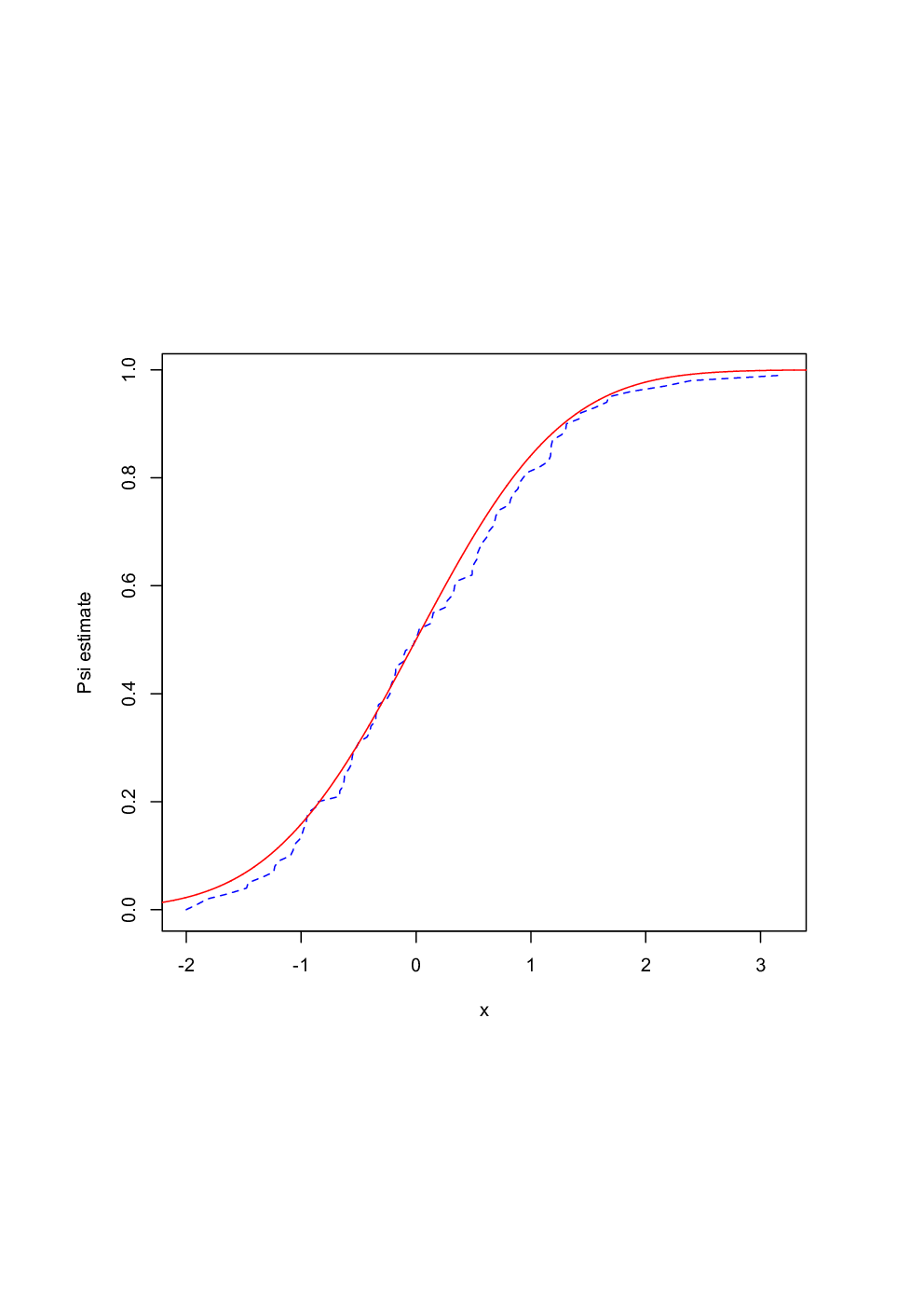
The shape parameter $\gamma$ is estimated via the Hill estimator (see e.g. Beirlant et al. (2004, Chapter 4)), which requires specifying how many upper order statistics will be used. This first threshold will be denoted by $k_{\gamma}$ in the following. Using the estimates of $\psi$ , $m$ , $a$ and $\Psi$ respectively defined by (10), (12), (13) and (17) also requires choosing a second threshold, which is the number of observations kept with largest first component, denoted by $k$ in Section 3. We have compared the theoretical value of $\Psi(\mu+\tau\,\cdot)$ with the estimate given by $\hat{\Psi}$ for different values of $\theta\in(0,1)$ and $\gamma\in(0,1/2)$ , sample size $n=10^{4}$ and different thresholds ( $k=200,500,1000,2000,3000$ and $k_{\gamma}=50,500$ ). Figure 1 illustrates the estimation of $\Psi$ via the nonparametric estimator $\hat{\Psi}$ defined by (17) for one sample.

Refer to caption — Figure 1: Estimation of $\Psi(\mu+\tau\,\cdot)$ via the nonparametric estimator $\hat{\Psi}$ for one sample ( $n=1000,k=300,k_{\gamma}=50$ ) of distribution with Fréchet margins of parameter $1/\gamma$ and Frank’s copula with parameter $\theta$ , for $\gamma=0.1$ and $\theta=0.3$ .

In each case listed above, 100 samples have been simulated, and for each of them, the $L^{1}$ -distance $\int|\hat{\Psi}(z)-\Psi(\mu+\tau z)|dz$ has been calculated. A summary of the results obtained is provided in Figure 2, which give the boxplots of the $L^{1}$ -distances for $\theta=0.3$ , $\gamma=0.1$ or $\gamma=0.4$ , and $n=10^{4}$ . The results obtained for other values of $\theta$ were very similar, so for brevity we do not present them.

A common feature of both plots of Figure 2 is that the results do not depend much on the choice of the threshold $k_{\gamma}$ , but are a bit more sensitive to the choice of the second threshold $k$ . Besides, the results show that the estimators provided in Section 3 perform well in a context that is rather general. Finally, these performances are better when the parameter $\gamma$ is smaller.

5.2 Goodness-of-fit test for the distribution $\Psi$

Assume that the hypotheses of Section 4 hold, so that the nonparametric estimation procedure described in Section 4.1 can be used. Three types of distributions are considered, each of them restricted to the positive quadrant for convenience. These distributions are:
(a) the elliptical distribution with radial survival function $P(R>t)=\mathrm{e}^{-t}$ , and Pearson correlation coefficient $\rho=0.5$ ;
(b) the distribution with radial representation $R(\cos[(\pi/2+\arcsin\rho)T-\arcsin\rho],\sin[(\pi/2+\arcsin\rho)T])$ , where $P(R>t)=\mathrm{e}^{-t^{2}/2}$ , $T$ has a non uniform concave density function $f_{T}(t)=4/\left\{\pi+\pi(2t-1)^{2}\right\}$ on $[0,1]$ , and $\rho=0.5$ ;
(c) the distribution with radial representation $R(\cos[(\pi/2+\arcsin\rho)T-\arcsin\rho],\sin[(\pi/2+\arcsin\rho)T])$ , where $P(R>t)=\mathrm{e}^{-t^{2}/2}$ , $T$ has a non uniform convex density function $f_{T}(t)=2-4/\left\{\pi(1+(2t-1)^{2}\right\}$ on $[0,1]$ , and $\rho=0.5$ .

Case (a) is an example of the standard elliptical case, for which estimation results already exist (see Abdous et al. (2008)), whereas (b) and (c) illustrate the situation where the density level lines are “asymptotically elliptic” (see Fougères and Soulier (2010)). In these three cases, $\Psi$ is the Normal distribution function (denoted by $\Phi$ ), and Assumption 6 is fulfilled with $\beta=2$ . Figure 3 illustrates the estimation of $\Psi$ via the nonparametric estimator $\check{\Psi}$ defined by (30) for one sample ( $n=1000,k=100$ ) of distribution (b).

The test statistic $T_{KS}$ of the Kolmogorov-Smirnov goodness-of-fit test performed here is defined by

\displaystyle T_{KS}=\sup_{y\in{\mathbb{R}}}\sqrt{k}|\check{\Psi}(y)-\Phi(y)|\;.

(47)

As shown in Section 4.1, $T_{KS}$ has asymptotically the same distribution as the random variable $Z$ defined in (34). Quantiles of this distribution have been obtained numerically and are listed in Table 1.

Table 1: Quantiles

q_{\alpha}

of order

1-\alpha

Z

$\alpha$	0.01	0.05	0.10	0.15	0.20	0.25
$q_{\alpha}$	1.598	1.297	1.174	1.076	1.029	0.980

We have compared these theoretical levels to the empirical levels obtained by simulation. In the three cases (a) to (c), 1000 samples of size $n=10^{3}$ , $10^{4}$ and $10^{5}$ , are simulated. The $k$ observations having the largest first component are kept, for three different values of $k$ , and the nonparametric estimate $\check{\Psi}$ given in (30) is computed with this reduced sample. The observed values of the test statistic $T_{KS}$ are compared to the quantiles listed in Table 1. For brevity, we present only the results corresponding to the two theoretical levels $\alpha=(0.05,0.1)$ . These empirical levels are shown in Table 2.

Table 2: Empirical levels

(\hat{\alpha}_{0.05},\hat{\alpha}_{0.1})

associated to theoretical levels

(0.05,0.1)

for the goodness-of-fit test with statistic

T_{KS}

. The original sample size is denoted by

n

, and the number of observations used for the estimation is denoted by

k

. Notation (a)–(c) refers to the three bivariate distributions listed above. The boldface characters point out the best result in each case.

\begin{array}[]{ccccc}n&k&{\mbox{\bf(a)}}&{\mbox{\bf(b)}}&{\mbox{\bf(c)}}\\ \hline\cr&50&{{\bf(0.053,0.095)}}&(0.031,0.066)&(0.027,0.050)\\ 1000&100&(0.140,0.231)&{{\bf(0.055,0.102)}}&{{\bf(0.04,0.085)}}\\ &150&(0.327,0.453)&(0.071,0.147)&(0.077,0.153)\\ \hline\cr&50&{(0.059,0.095)}&(0.03,0.061)&(0.028,0.045)\\ 10000&100&{{\bf(0.052,0.099)}}&(0.038,0.07)&{\bf(0.038,0.088)}\\ &200&{(0.101,0.183)}&{\bf(0.054,0.096)}&{(0.065,0.125)}\\ \hline\cr&100&{\bf(0.051,0.082)}&(0.037,0.075)&{\bf(0.044,0.071)}\\ 100000&200&(0.080,0.133)&{(0.041,0.087)}&{(0.0795,0.128)}\\ &500&{(0.140,0.257)}&{\bf(0.05,0.103)}&(0.20,0.298)\\ \hline\cr\end{array}

A common feature for the three distributions is that the results are rather sensitive to the reduced number of observations $k$ . However, the value of $k$ leading to the best adequation between empirical and theoretical levels is rather stable in most cases studied ( $k=100$ in two thirds of the cases).

5.3 Semiparametric estimation of the conditional quantile function

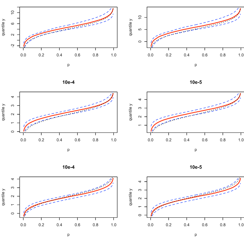
Assume that Assumptions 1, 4, 6 and equation (35) hold and that the limiting distribution $\Psi$ is the standard Gaussian distribution $\Phi$ . The small sample behavior of the semiparametric estimator $\hat{y}_{n}(p)$ of the quantile function $\theta^{\leftarrow}(x_{n},p)$ defined by Equation (46) is illustrated in Figure 4 for the three distributions presented in Section 5.2. In each case, 100 samples of size 10000 are simulated. A proportion of 1% of the observations is used, which are the 100 observations with largest first component. For each sample, the conditional quantile function $\theta^{\leftarrow}(x,p)$ is estimated for two values of $x$ corresponding to the theoretical $X$ -quantiles of order $1-\epsilon$ , where $\epsilon=10^{-4}$ and $\epsilon=10^{-5}$ . Figure 4 summarizes the quality of these estimations by showing the median, and the 2.5%- and 97.5%-quantiles of $\hat{y}_{n}(p)$ for the two fixed values of $x$ specified above.

The estimation results are globally good, and the best ones are obtained for cases (a) and (c), see rows 1 and 3 of Figure 4. Besides, one can observe a slight improvement as the conditioning event becomes more extreme.

These empirical interval confidence compare well with those obtained by applying the central limit theorem of Corollary 16. We do not show them on Figure 4 for the sake of clarity.

6 Data analysis

To illustrate the use of the new procedures, and more specifically the Kolmogorov-Smirnov goodness-of-fit test proposed in Section 4.1, the hypothesis of $\Psi=\Phi$ , where $\Phi$ is the standard Gaussian cdf, is tested using the series of monthly returns for the 3M stock and the Dow Jones Industrial Average from January 1970 to January 2008 ( $n=457$ values). These data were used by Levy and Duchin (2004) and revisited by Abdous et al. (2008). In the latter paper, the hypothesis of bivariate ellipticity was accepted through a test of elliptical symmetry proposed by Huffer and Park (2007) and the contagion from the Dow Jones to the 3M stock was tested. As shown in Abdous et al. (2005), ellipticity implies that Condition (1) holds and that the limiting distribution is the Gaussian law. The present procedure allows to test for the Gaussian conditional limit law without assuming ellipticity, but the weaker assumption (1). The observed values of the test statistic $T_{KS}$ defined by (47) in terms of different choices of threshold $k$ (or equivalently in terms of the proportion $r$ of observations used, $k=nr$ ) are summarized in Table 3. According to Table 1, all these observed values correspond to a $p$ -value greater than 0.25, which leads to accept the hypothesis $\Psi=\Phi$ .

Table 3: Observed values

t_{KS}

of the test statistic

T_{KS}

defined by (47) in terms of the proportion

r

or number

k

of observations used.

$r$	0.05	0.10	0.15	0.20
$k$	22	45	68	91
$t_{KS}$	0.842	0.847	0.777	0.948

7 Proofs

Proof of Proposition 3.

By Proposition 2, the weak convergence of $\tilde{\nu}_{n}$ to $\nu$ implies that for any compact set $K$ of $(-1/\gamma,\infty)\times(-\infty,\infty)$ such that $\nu(\partial K)=0$ and any function $h$ , it holds that

\displaystyle\lim_{n\to\infty}\iint_{K}h(x,y)\tilde{\nu}_{n}(\mathrm{d}x,\mathrm{d}y)=\iint_{K}h(x,y)\nu(\mathrm{d}x,\mathrm{d}y)\ \mbox{ in probability.}

For $\epsilon,M>0$ , $\epsilon<1/\gamma$ , define $K=[-\epsilon,M]\times[-M,M]$ and $K^{c}=[-\epsilon,\infty)\times(-\infty,\infty)\setminus K$ . Let $h$ be a nonnegative function on $[-\epsilon,\infty)\times(-\infty,\infty)$ such that $h(x,y)\leq C(|x|\vee 1)^{q^{*}-1}(|y|\vee 1)^{p^{*}-1}$ . We must prove that

\displaystyle\limsup_{M\to\infty}\lim_{n\to\infty}\iint_{K^{c}}h(x,y)\tilde{\nu}_{n}(\mathrm{d}x,\mathrm{d}y)=0\;,

(48)

in probability. Since

\displaystyle\mathbb{E}\left[\iint_{K^{c}}h(x,y)\tilde{\nu}_{n}(\mathrm{d}x,\mathrm{d}y)\right]=\iint_{K^{c}}h(x,y)\nu_{n/k}(x,y)\;,

Assumption 2 implies that

\lim_{M\to\infty}\limsup_{n\to\infty}\mathbb{E}\left[\iint_{K^{c}}h(x,y)\tilde{\nu}_{n}(\mathrm{d}x,\mathrm{d}y)\right]\\ =\lim_{M\to\infty}\limsup_{n\to\infty}\iint_{K^{c}}h(x,y)\nu_{n/k}(\mathrm{d}x,\mathrm{d}y)=\lim_{M\to\infty}\iint_{K^{c}}h(x,y)\nu(\mathrm{d}x,\mathrm{d}y)\;.

This yields (48) and concludes the proof of Proposition 3. ∎

Proof of Proposition 4.

Assumption 2 and (Resnick, 1986, Proposition 5.3) imply that the sequence of point processes

\displaystyle\sum_{k=1}^{n}\delta_{\frac{X_{k}-b(n)}{\psi\circ b(n)},\frac{Y_{k}-m\circ b(n)}{a\circ b(n)}}

converges weakly to a Poisson point process on $(-1/\gamma,\infty]\times(-\infty,\infty)$ with intensity measure $\nu$ . This implies that the vector $({(X_{(n:n)}-b(n))}/{\psi\circ b(n)},({Y_{[n:n]}-m\circ b(n)})/{a\circ b(n)})$ converges weakly to the distribution $F$ defined in (1).

∎

Proof of Proposition 5.

Write

\displaystyle\frac{\hat{m}(X_{(n:n-k)})-m\circ b(n/k)}{a\circ b(n/k)}=\frac{S_{n}}{T_{n}}\;,

with

	$\displaystyle S_{n}$	$\displaystyle=\frac{1}{k}\sum_{i=1}^{k}\frac{Y_{[n:n-i+1]}-m\circ b(n/k)}{a\circ b(n/k)}\;\frac{X_{(n:n-i+1)}-X_{(n:n-k)}}{\psi\circ b(n/k)}\;,$
	$\displaystyle T_{n}$	$\displaystyle=\frac{1}{k}\sum_{i=1}^{k}\frac{X_{(n:n-i+1)}-X_{(n:n-k)}}{\psi\circ b(n/k)}\;.$

We have already seen that $T_{n}$ converges weakly to $1/(1-\gamma)$ . Recall that we have defined

\displaystyle\tilde{x}_{n}=\frac{X_{(n:n-k)}-b(n/k)}{\psi\circ b(n/k)}\;.

By definition of $\tilde{\nu}_{n}$ , we have, (with $x_{+}=\sup(x,0)$ for any real number $x$ )

	$\displaystyle S_{n}$	$\displaystyle=\frac{1}{k}\sum_{i=1}^{n}\frac{Y_{i}-m\circ b(n/k)}{a(X_{(n:n-k)})}\;\left\{\frac{X_{i}-b(n/k)}{\psi\circ b(n/k)}-\tilde{x}_{n}\right\}_{+}=\int_{\tilde{x}_{n}}^{\infty}\int_{-\infty}^{\infty}(x-\tilde{x}_{n})y\,\tilde{\nu}_{n}(\mathrm{d}x,\mathrm{d}y)$
		$\displaystyle=\int_{0}^{\infty}\int_{-\infty}^{\infty}xy\,\tilde{\nu}_{n}(\d{x},\mathrm{d}y)-\int_{0}^{\tilde{x}_{n}}\int_{-\infty}^{\infty}xy\,\tilde{\nu}_{n}(\mathrm{d}x,\mathrm{d}y)-\tilde{x}_{n}\int_{\tilde{x}_{n}}^{\infty}\int_{-\infty}^{\infty}y\,\tilde{\nu}_{n}(\mathrm{d}x,\mathrm{d}y)\;.$		(49)

By Proposition 3, the first term in (49) converges to $\mu/(1-\gamma)$ . Under Assumption 1, it is well known that $\tilde{x}_{n}=o_{P}(1)$ . Cf. De Haan and Ferreira (2006, Theorem 2.2.1). This and Assumption 2 imply that the last two terms in (49) are $o_{P}(1)$ . Thus $S_{n}$ converges weakly to $\mu/(1-\gamma)$ by Proposition 3. If $m(x)=\rho x$ , then $\hat{\rho}-\rho\sim X_{(n:n-k)}^{-1}a(X_{(n:n-k)})\mu$ which converges to 0 if $a(x)=o(x)$ or if $\mu=0$ and $a(x)=O(x)$ . ∎

Proof of Proposition 6.

We show that $\hat{a}^{2}(X_{(n:n-k)})/a^{2}\circ b(n/k)$ converges weakly to 1. Recall that $\xi_{n}=\{\hat{m}(X_{(n:n-k)})-m\circ b(n/k)\}/a\circ b(n/k)$ . By Proposition 5, $\xi_{n}=o_{P}(1)$ , and noting that $\tilde{\nu}_{n}\{[\tilde{x}_{n},\infty]\times[-\infty,\infty]\}=1$ , where $\tilde{\nu}_{n}$ and $\tilde{x}_{n}$ are respectively defined by (5) and (16), we have

	$\displaystyle\frac{\hat{a}^{2}(X_{(n:n-k)})}{a^{2}\circ b(n/k)}$	$\displaystyle=\frac{1}{k}\sum_{i=1}^{n}\left\{\frac{Y_{i}-m\circ b(n/k)}{a\circ b(n/k)}-\xi_{n}\right\}^{2}\mathbf{1}_{\{\frac{X_{i}-b(n/k)}{\psi\circ b(n/k)}\geq\tilde{x}_{n}\}}$
		$\displaystyle=\int_{\tilde{x}_{n}}^{\infty}\int_{-\infty}^{\infty}(y-\xi_{n})^{2}\,\tilde{\nu}_{n}(\mathrm{d}x,\mathrm{d}y)$
		$\displaystyle=\int_{\tilde{x}_{n}}^{\infty}\int_{-\infty}^{\infty}y^{2}\,\tilde{\nu}_{n}(\mathrm{d}x,\mathrm{d}y)-2\xi_{n}\int_{\tilde{x}_{n}}^{\infty}\int_{-\infty}^{\infty}y\,\tilde{\nu}_{n}(\mathrm{d}x,\mathrm{d}y)+\xi_{n}^{2}$
		$\displaystyle=\int_{0}^{\infty}\int_{-\infty}^{\infty}y^{2}\,\tilde{\nu}_{n}(\d{x},\mathrm{d}y)+o_{P}(1)\;.$

Thus $\hat{a}(X_{(n:n-k)})/a\circ b(n/k)$ converges weakly to 1 by Proposition 3 and equation (8). ∎

Proof of Proposition 8.

Note first that assumption (20) implies that $k$ is an intermediate sequence, i.e. $n/k\to 0$ , since $\lim_{t\to\infty}c\circ b(t)=0$ . We start by proving the convergence of the finite dimensional distributions of $W_{n}$ . Denote $G_{n}(x,y)=\nu_{n}((x,\infty)\times(-\infty,y])$ , $G(x,y)=\nu((x,\infty)\times(-\infty,y])$ , $\tilde{X}_{i}=\{X_{i}-b(n/k)\}/\psi\circ b(n/k)$ , $\tilde{Y}_{i}=\{Y_{i}-m\circ b(n/k)\}/a\circ b(n/k)$ and

	$\displaystyle\xi_{n,i}(x,y)$	$\displaystyle=k^{-1/2}\{\mathbf{1}_{\{\tilde{X}_{i}>x\,,\;\tilde{Y}_{i}\leq y\}}-\mathbb{P}(\tilde{X}_{i}>x\;,\tilde{Y}_{i}\leq y)\}$
		$\displaystyle=k^{-1/2}\{\mathbf{1}_{\{\tilde{X}_{i}>x\,,\;\tilde{Y}_{i}\leq y\}}-kn^{-1}G_{n/k}(x,y)\}\;.$

Then for each $n$ , the random variables $\xi_{n,i}$ , $1\leq i\leq n$ are i.i.d.,

\displaystyle\mathrm{cov}(\xi_{n,i}(x,y),\xi_{n,i}(x^{\prime},y^{\prime}))=\frac{1}{n}G_{n/k}(x\vee x^{\prime},y\wedge y^{\prime})-\frac{k}{n^{2}}G_{n/k}(x,y)G_{n/k}(x^{\prime},y^{\prime})\;,

and

\displaystyle W_{n}(x,y)=\sum_{i=1}^{n}\xi_{n,i}(x,y)+k^{1/2}\{G_{n/k}(x,y)-G(x,y)\}\;.

Assumption 3 and (20) imply that $k^{1/2}(G_{n/k}-G)$ converges to zero locally uniformly. The Lindeberg central limit theorem (cf. Araujo and Giné (1980)) and (20) yield the convergence of finite dimensional distributions of $\sum_{i=1}^{n}\xi_{n,i}(x,y)$ to the Gaussian process with covariance defined by (21).

Let $\mathcal{K}$ be a compact set of $(-1/\gamma,\infty)\times(-\infty,\infty)$ . The tightness of the sequence of processes $\{\sum_{i=1}^{n}\xi_{n,i}(x,y),(x,y)\in\mathcal{K}\}$ is obtained by applying (van der Vaart and Wellner, 1996, Example 2.11.8) with $c_{n,i}=1/\sqrt{k}$ , $P_{n,i}=P_{n}=\mathbb{P}((\tilde{X}_{i},\tilde{Y}_{i})\in\cdot)$ and the set of functions $\mathcal{F}$ is the set of indicators $\mathbf{1}_{\{(x,\infty)\times(-\infty,y]\}}$ for $(x,y)\in\mathcal{K}$ . The conditions of Example 2.11.8 are satisfied, since $\max_{1\leq i\leq n}|c_{n,i}|\to 0$ trivially, and

\displaystyle\sum_{i=1}^{n}c_{n,i}^{2}P_{n,i}=\frac{n}{k}P_{n}\to F\;,

by Assumption 1 and Proposition 2. Finally, the class $\mathcal{F}$ satisfies the uniform entropy condition, as shown in (van der Vaart and Wellner, 1996, Example 2.5.4).

This proves the convergence of the sequence of processes $\sum_{i=1}^{n}\xi_{n,i}$ to $W$ uniformly on compact sets of $(-1/\gamma,\infty)\times(-\infty),\infty)$ .

We now prove the second part of Proposition 8. Let $h$ be a $C^{\infty}$ function with compact support in $(-1/\gamma,\infty)\times(-\infty,\infty)$ . The weak convergence of $W_{n}$ in $\mathcal{D}((-1/\gamma,\infty)\times(-\infty,\infty))$ implies that $\iint h(x,y)W_{n}(x,y)\,\mathrm{d}x\,\mathrm{d}y$ converges weakly to $\iint h(x,y)W(x,y)\,\mathrm{d}x\,\mathrm{d}y$ . Thus, by integration by parts, it also holds that $\iint h(x,y)W_{n}(\mathrm{d}x,\mathrm{d}y)$ converges weakly to $\iint h(x,y)W(\mathrm{d}x,\mathrm{d}y)$ . Let $\epsilon\in(0,1/\gamma)$ and define $A=[-\epsilon,\infty)\times(-\infty,\infty)$ . Let $g$ be a measurable function defined on $A$ such that $|g(x,y)|^{2}\leq C(|x|\vee 1)^{p^{\dagger}}(|y|\vee 1)^{q^{\dagger}}$ . Then, for all $\epsilon>0$ , there exists a $C^{\infty}$ function $h$ with compact support in $A$ such that $\int_{A}(g-h)^{2}\,\mathrm{d}\nu\leq\epsilon$ . Then,

\displaystyle\int_{A}g\,\mathrm{d}\tilde{\mu}_{n}=\int_{A}h\,\mathrm{d}\tilde{\mu}_{n}+\int_{A}(g-h)\,\mathrm{d}\tilde{\mu}_{n}\;.

The first term in the right hand side converges weakly to $W(h)$ and we prove now that the second one converges in probability to 0. Denote $u=g-h$ and

\displaystyle\mu_{n}=k^{1/2}\{\nu_{n/k}-\nu\}\;.

Then,

\displaystyle\int_{A}u\,\mathrm{d}\tilde{\mu}_{n}=k^{-1/2}\sum_{i=1}^{n}\{u(\tilde{X}_{i},\tilde{Y}_{i})-\mathbb{E}[u(\tilde{X}_{i},\tilde{Y}_{i})]\}+\int_{A}u\,\mathrm{d}\mu_{n}\;.

By definition, for any function $v$ , $\mathbb{E}[v(\tilde{X}_{1})]=kn^{-1}\int v\,\mathrm{d}\nu_{n/k}$ , thus

\displaystyle\mathbb{E}\left[\left(\int_{A}u\,\mathrm{d}\tilde{\mu}_{n}\right)^{2}\right]\leq\int_{A}u^{2}\,\mathrm{d}\nu_{n/k}+\left\{\int_{A}u\,\mathrm{d}\mu_{n}\right\}^{2}\;.

By assumption on $g$ , and since $h$ has compact support, it also holds that $u^{2}(x,y)\leq C(|x|\vee 1)^{p^{\dagger}}(|y|\vee 1)^{q^{\dagger}}$ . Thus, by Assumption 3 and (20), it holds that $\lim_{n\to\infty}\int_{A}u\,\mathrm{d}\mu_{n}=0$ and $\lim_{n\to\infty}\int_{A}u^{2}\,\mathrm{d}\nu_{n}=\int_{A}u^{2}\,\mathrm{d}\nu$ . Thus

\displaystyle\limsup_{n\to\infty}\mathbb{E}\left[\left(\int_{A}u\,\mathrm{d}\tilde{\mu}_{n}\right)^{2}\right]\leq\int_{A}u^{2}\,\mathrm{d}\nu\leq\epsilon\;.

Taking into account that $\mathrm{var}(W(g)-W(h))=\mathrm{var}(W(g-h))=\int_{A}(g-h)^{2}\,\mathrm{d}\nu\leq\epsilon$ , we conclude that $W_{n}(g)$ converges weakly to $W(g)$ and that $\mathbb{E}[W^{2}(g)]=\int g^{2}\mathrm{d}\nu$ . The joint convergence of $W_{n}(g_{1}),\dots,W_{n}(g_{k})$ is obtained by the Cramer-Wold device, and by linearity of $W_{n}$ and $W$ , this is reduced to the one-dimensional convergence. ∎

Proof of Corollary 9.

We prove separately the claimed limit distributions. The joint convergence is obvious. We start with $\tilde{x}_{n}$ , defined in (16). Denote $\mathbb{G}_{n}(x)=\tilde{\nu}_{n}((x,\infty)\times(-\infty,+\infty))$ . By Proposition 8, $k^{1/2}(\mathbb{G}_{n}-\bar{P}_{\gamma})$ converges weakly in $\mathcal{D}$ to the process $B\circ\bar{P}_{\gamma}$ , where $B$ is a standard Brownian motion on $[0,1]$ . By Vervaat’s Lemma (De Haan and Ferreira, 2006, Lemma A.0.2), $k^{1/2}\{\mathbb{G}_{n}^{\leftarrow}-\bar{P}_{\gamma}^{\leftarrow}\}$ jointly converges weakly in $\mathcal{D}$ to $-(\bar{P}_{\gamma}^{\leftarrow})^{\prime}B$ . Since $\mathbb{G}_{n}^{\leftarrow}(1)=\tilde{x}_{n}$ , $\bar{P}_{\gamma}^{\leftarrow}(1)=0$ and $(\bar{P}_{\gamma}^{\leftarrow})^{\prime}(1)=-1$ , we get the claimed limit distribution for $k^{1/2}\tilde{x}_{n}$ .

We now consider $\xi_{n}$ , defined in (16). By definition,

	$\displaystyle\xi_{n}$	$\displaystyle=\frac{\sum_{i=1}^{k}\{X_{(n:n-i+1)}-X_{(n:n-k)}\}\{Y_{[n:n-i+1]}-m\circ b(n/k)\}}{k\psi\circ b(n/k)a\circ b(n/k)}$
		$\displaystyle\hskip 142.26378pt\div\ \frac{\sum_{i=1}^{k}\{X_{(n:n-i+1)}-X_{(n:n-k)\}}}{k\psi\circ b(n/k)}$
		$\displaystyle=\frac{\int_{\tilde{x}_{n}}^{\infty}\int_{-\infty}^{\infty}(x-\tilde{x}_{n})y\tilde{\nu}_{n}(\mathrm{d}x,\mathrm{d}y)}{\int_{\tilde{x}_{n}}^{\infty}\int_{-\infty}^{\infty}(x-\tilde{x}_{n})\tilde{\nu}_{n}(\mathrm{d}x,\mathrm{d}y)}\;.$

Since $\mu=0$ by assumption, we obtain

\displaystyle k^{1/2}\xi_{n}=\frac{\int_{\tilde{x}_{n}}^{\infty}\int_{-\infty}^{\infty}(x-\tilde{x}_{n})y\tilde{\mu}_{n}(\mathrm{d}x,\mathrm{d}y)}{\int_{\tilde{x}_{n}}^{\infty}\int_{-\infty}^{\infty}(x-\tilde{x}_{n})\tilde{\nu}_{n}(\mathrm{d}x,\mathrm{d}y)}\;.

Since $\tilde{x}_{n}=O_{P}(k^{-1/2})$ , it is easily seen that

\displaystyle k^{1/2}\xi_{n}=\frac{\int_{0}^{\infty}\int_{-\infty}^{\infty}xy\tilde{\mu}_{n}(\mathrm{d}x,\mathrm{d}y)+o_{P}(1)}{\int_{0}^{\infty}\int_{-\infty}^{\infty}x\tilde{\nu}_{n}(\mathrm{d}x,\mathrm{d}y)+o_{P}(1)}\;.

Applying Propositions 3 and 8, we obtain that $k^{1/2}\xi_{n}$ converges weakly to $(1-\gamma)W(g_{1,1})$ . Consider now $\hat{a}(X_{(n:n-k)})$ . As in the proof of Proposition 6, we write

\displaystyle\frac{\hat{a}^{2}(X_{(n:n-k)})}{a^{2}\circ(n/k)}

\displaystyle=\int_{\tilde{x}_{n}}^{\infty}\int_{-\infty}^{\infty}y^{2}\tilde{\nu}_{n}(\mathrm{d}x,\mathrm{d}y)-2\xi_{n}\int_{\tilde{x}_{n}}^{\infty}\int_{-\infty}^{\infty}y\tilde{\nu}_{n}(\mathrm{d}x,\mathrm{d}y)+\xi_{n}^{2}\;,

and since $\tilde{x}_{n}=O_{P}(k^{-1/2})$ and $\xi_{n}=O_{P}(k^{-1/2})$ , we get

\displaystyle k^{1/2}\left\{\frac{\hat{a}^{2}(X_{(n:n-k)})}{a^{2}\circ b(n/k)}-1\right\}=\int_{0}^{\infty}\int_{-\infty}^{\infty}y^{2}\tilde{\mu}_{n}(\d{x},\mathrm{d}y)+o_{P}(1)\;.

Proposition 8 and the delta method yield that $k^{1/2}\{{\hat{a}(X_{(n:n-k)})}/{a\circ b(n/k)}-1\}$ converges weakly to $\frac{1}{2}W(g_{0,2})$ . ∎

Proof of Proposition 15.

The asymptotic normality of $\hat{\beta}_{k}$ is proved (under more general conditions) in Gardes and Girard (2006, Corollary 1). Consider now $\breve{a}_{k_{1}}(x_{n})$ . By (35) and (37),

\displaystyle a(x)=a(X_{(n:n-k_{1})})\left(\frac{x}{X_{(n:n-k_{1})}}\right)^{1-\beta/2}\;,

thus, by (39), we obtain

\displaystyle\frac{\breve{a}_{k_{1}}(x_{n})}{a(x_{n})}=\frac{\check{a}_{k_{1}}(X_{(n:n-k_{1})})}{a(X_{(n:n-k_{1})})}\;X_{(n:n-k_{1})}^{(\hat{\beta}_{k}-\beta)/2}\;x_{n}^{(\beta-\hat{\beta}_{k})/2}\;.

Decomposing further, we get

$\displaystyle\frac{\breve{a}_{k_{1}}(x_{n})}{a(x_{n})}-1$	$\displaystyle=\left\{\frac{\check{a}_{k_{1}}(X_{(n:n-k_{1})})}{a(X_{(n:n-k_{1})})}-1\right\}X_{(n:n-k_{1})}^{(\hat{\beta}_{k}-\beta)/2}\;x_{n}^{(\beta-\hat{\beta}_{k})/2}$	(50)
	$\displaystyle+\left\{X_{(n:n-k_{1})}^{(\hat{\beta}_{k}-\beta)/2}-1\right\}\left\{x_{n}^{(\beta-\hat{\beta}_{k})/2}-1\right\}$	(51)
	$\displaystyle+X_{(n:n-k_{1})}^{(\hat{\beta}_{k}-\beta)/2}-1+x_{n}^{(\beta-\hat{\beta}_{k})/2}-1\;.$	(52)

Since $\hat{\beta}_{k}-\beta=O_{P}(k^{-1/2})$ , $\log(x_{n})=o(k^{1/2})$ and $k/k_{1}\to 0$ , we obtain

	$\displaystyle x_{n}^{(\beta-\hat{\beta}_{k})/2}-1$	$\displaystyle\sim(\beta-\hat{\beta}_{k})\log(x_{n})/2\;,$
	$\displaystyle X_{(n:n-k_{1})}^{(\beta-\hat{\beta}_{k})/2}-1$	$\displaystyle\sim(\beta-\hat{\beta}_{k})\log(X_{(n:n-k_{1})})/2\sim(\beta-\hat{\beta}_{k})\log(b(n/k_{1}))/2\;,$

where the equivalence relations above hold in probability. Thus, by the first part of Proposition 15 and (43) the product in (51) is $O_{P}(k^{-1}\log^{2}(x_{n}))=o_{P}(k^{-1/2}\log(x_{n}))$ by (44). By Theorem 14, $\check{a}_{k_{1}}(X_{(n:n-k_{1})})/a(X_{(n:n-k_{1})})-1=O_{P}(k_{1}^{-1/2})$ , thus the term in the right hand side of (50) is $O_{P}(k_{1}^{-1/2})=o_{P}(k^{-1/2}\log(x_{n}))$ since $k/k_{1}\to 0$ . Altogether, these bounds yields,

\displaystyle\frac{k^{1/2}}{\log(x_{n})}\left\{\frac{\breve{a}_{k_{1}}(x_{n})}{a(x_{n})}-1\right\}=k^{1/2}(\beta-\hat{\beta}_{k})+o_{P}(1)\;,

and the proof follows from the asymptotic normality of $k^{1/2}(\beta-\hat{\beta}_{k})$ . ∎

Proof of Corollary 16.

Define $\tilde{y}_{n}=\rho x_{n}+a(x_{n})\Psi^{-1}(p)$ . Then

	$\displaystyle\hat{y}_{n}-y_{n}$	$\displaystyle=\hat{y}_{n}-\tilde{y}_{n}+\tilde{y}_{n}-y_{n}$
		$\displaystyle=(\hat{\rho}_{k_{1}}-\rho)x_{n}+(\breve{a}_{k_{1}}(x_{n})-a(x_{n}))\Psi^{-1}(p)+\tilde{y}_{n}-y_{n}\;.$

In order to study $\tilde{y}_{n}-y_{n}$ , denote $z_{n}=(y_{n}-\rho x_{n})/a(x_{n})$ . Then $\lim_{n\to\infty}z_{n}=\Psi^{-1}(p)$ . Indeed, if the sequence $z_{n}$ is unbounded, then it tends to infinity at least along a subsequence. Choose $z>\Psi^{-1}(p)$ . Then, for large enough $n$ ,

	$\displaystyle p$	$\displaystyle=\mathbb{P}(Y\leq\rho x_{n}+a(x_{n})z_{n}\mid X>x_{n})\geq\mathbb{P}(Y\leq\rho x_{n}+a(x_{n})z\mid X>x_{n})$
		$\displaystyle\to\Psi(z)>p\;.$

Thus the sequence $z_{n}$ is bounded, and if it converges to $z$ (along a subsequence), it necessarily holds that $\Psi(z)=p$ , thus $z_{n}$ converges to $\Psi^{-1}(p)$ . Since we have assumed that $a(x)=o(x)$ , this implies that $y_{n}\sim\rho x_{n}$ and

\displaystyle\frac{\tilde{y}_{n}-y_{n}}{y_{n}}\sim\frac{a(x_{n})\{\Psi^{-1}(p)-z_{n}\}}{\rho x_{n}}\to 0\;.

Moreover, since $\Psi^{\prime}\circ\Psi^{-1}(p)>0$ , by a first order Taylor expansion, we have

\displaystyle\Psi^{-1}(p)-z_{n}=\frac{1}{\Psi^{\prime}(\xi_{n})}\{\theta(x_{n},y_{n})-\Psi(z_{n})\}\;,

where $\xi_{n}=\Psi^{-1}(p)+u\{z_{n}-\Psi^{-1}(p)\}$ for some $u\in(0,1)$ . By Assumption 3, $\|\theta(x_{n},\rho x_{n}+a(x_{n})\cdot)-\Psi\|_{\infty}=O(c\circ b(n))$ . Since we have already shown that $z_{n}$ converges to $\Psi^{-1}(p)$ , $1/\Psi^{\prime}(\xi_{n})$ is bounded for large enough $n$ , so $\Psi^{-1}(p)-z_{n}=O(c\circ b(n))$ . Thus, by (41) (with $c$ instead of $\tilde{c}$ ), we get

\displaystyle\frac{k^{1/2}x_{n}}{\log(x_{n})a(x_{n})}\frac{\tilde{y}_{n}-y_{n}}{y_{n}}=O\left(\frac{k^{1/2}c\circ b(n)}{\log(x_{n})}\right)=o\left(\frac{k_{1}^{1/2}c\circ b(n)}{\log(x_{n})}\right)=o(1)\;.

Next, by definition, and since $y_{n}\sim\rho x_{n}$ and $a(x_{n})=o(x_{n})$ , we have

\displaystyle\frac{\hat{y}_{n}-\tilde{y}_{n}}{y_{n}}\sim\frac{\hat{\rho}_{k_{1}}-\rho}{\rho}+\frac{a(x_{n})\Psi^{-1}(p)}{\rho x_{n}}\left\{\frac{\breve{a}_{k_{1}}(x_{n})}{a(x_{n})}-1\right\}\;.

Thus,

\displaystyle\frac{k^{1/2}}{\log(x_{n})}\frac{x_{n}}{a(x_{n})}\frac{\hat{y}_{n}-\tilde{y}_{n}}{y_{n}}

\displaystyle\sim\frac{k^{1/2}x_{n}(\hat{\rho}_{k_{1}}-\rho)}{\rho a(x_{n})\log(x_{n})}+\frac{\Psi^{-1}(p)}{\rho}\frac{k^{1/2}}{\log(x_{n})}\left\{\frac{\breve{a}_{k_{1}}(x_{n})}{a(x_{n})}-1\right\}\;.

The first term in the right-hand side tends to zero by Theorem 14 and the assumptions on the sequences $k_{1}$ , $k$ and $x_{n}$ . The second term converges weakly to a centered Gaussian law with variance $\{\Psi^{-1}(p)/(\rho\beta)\}^{2}$ by Proposition 15. In the case $\Psi^{-1}(p)=0$ , the main term is the first one in the right-hand side of the last display, and we conclude by applying Theorem 14. ∎

References

Abdous et al. (2005) Belkacem Abdous, Anne-Laure Fougères, and Kilani Ghoudi. Extreme behaviour for bivariate elliptical distributions. Revue Canadienne de Statistique, 33(2):1095–1107, 2005.
Abdous et al. (2008) Belkacem Abdous, Anne-Laure Fougères, Kilani Ghoudi, and Philippe Soulier. Estimation of bivariate excess probabilities for elliptical models. Bernoulli, 14(4):1065–1088, 2008.
Alink et al. (2004) Stan Alink, Matthias Löwe, and Mario V. Wüthrich. Diversification of aggregate dependent risks. Insurance Math. Econom., 35(1):77–95, 2004. ISSN 0167-6687.
Araujo and Giné (1980) Aloisio Araujo and Evarist Giné. The central limit theorem for real and Banach valued random variables. John Wiley & Sons, New York-Chichester-Brisbane, 1980. Wiley Series in Probability and Mathematical Statistics.
Asimit et al. (2010) Alexandru V. Asimit, Deyuan Li, and Liang Peng. Pitfalls in using Weibull tailed distributions. J. Statist. Plann. Inference, 140(7):2018–2024, 2010.
Balkema and Embrechts (2007) Guus Balkema and Paul Embrechts. High risk scenarios and extremes. A geometric approach. Zurich Lectures in Advanced Mathematics. Zürich: European Mathematical Society, 2007.
Barbe (2003) Philippe Barbe. Approximation of integrals over asymptotic sets with applications to probability and statistics. http://arxiv.org/abs/math/0312132, 2003.
Beirlant et al. (2004) Jan Beirlant, Yuri Goegebeur, Jozef Teugels, and Johan Segers. Statistics of extremes. Wiley Series in Probability and Statistics. John Wiley & Sons Ltd., Chichester, 2004.
Berman (1982) Simeon M. Berman. Sojourns and extremes of stationary processes. Annals of Probability, 10(1):1–46, 1982.
Berman (1992) Simeon M. Berman. Sojourns and extremes of stochastic processes. The Wadsworth & Brooks/Cole Statistics/Probability Series. Wadsworth & Brooks/Cole Advanced Books & Software, Pacific Grove, CA, 1992.
Bradley and Taqqu (2004) Brendan O. Bradley and Murad S. Taqqu. Framework for analyzing spatial contagion between financial markets. Finance Letters, 2(6):8–16, 2004.
Das and Resnick (2009) Bikramjit Das and Sidney I. Resnick. Detecting a conditional extreme value model. To appear in Extremes, 2009. DOI:10.1007/s10687-009-0097-3.
Das and Resnick (2010) Bikramjit Das and Sidney I. Resnick. Conditioning on an extreme component: Model consistency and regular variation on cones. To appear in Bernoulli, 2010.
Davydov and Egorov (2000) Youri Davydov and Vladimir A. Egorov. Functional limit theorems for induced order statistics. Mathematical Methods of Statistics, 9(3):297–313, 2000.
De Haan and Ferreira (2006) Laurens De Haan and Ana Ferreira. Extreme value theory. An introduction. Springer Series in Operations Research and Financial Engineering. New York, NY: Springer, 2006.
de Haan and Resnick (1993) Laurens de Haan and Sidney I. Resnick. Estimating the limit distribution of multivariate extremes. Communications in Statistics. Stochastic Models, 9(2):275–309, 1993.
Eddy and Gale (1981) William F. Eddy and James D. Gale. The convex hull of a spherically symmetric sample. Advances in Applied Probability, 13(4):751–763, 1981.
Fougères and Soulier (2010) Anne-Laure Fougères and Philippe Soulier. Limit conditional distributions for bivariate vectors with polar representation. Stochastic models, 26(1):54–77, 2010.
Gardes and Girard (2006) Laurent Gardes and Stéphane Girard. Comparison of Weibull tail-coefficient estimators. REVSTAT, 4(2):163–188, 2006.
Hashorva (2006) Enkelejd Hashorva. Gaussian approximation of conditional elliptic random vectors. Stoch. Models, 22(3):441–457, 2006.
Hashorva (2007) Enkelejd Hashorva. Asymptotic properties of type I elliptical random vectors. Extremes, 10:175–206, 2007.
Hashorva (2008) Enkelejd Hashorva. Conditional limiting distribution of beta-independent random vectors. Journal of Multivariate Analysis, 99(7):1438–1459, 2008.
Hashorva (2009a) Enkelejd Hashorva. Conditional limit results for type I polar distributions. Extremes, 12:239–263, 2009a.
Hashorva (2009b) Enkelejd Hashorva. Conditional limits of $w_{p}$ -scale mixture distributions. Journal of Statistical Planning and Inference, 139:3501–3511, 2009b.
Hashorva et al. (2007) Enkelejd Hashorva, Samuel Kotz, and Alfred Kume. $L_{p}$ -norm generalised symmetrised Dirichlet distributions. Albanian Journal of Mathematics, 1(1):31–56 (electronic), 2007.
Heffernan and Resnick (2007) Janet E. Heffernan and Sidney I. Resnick. Limit laws for random vectors with an extreme component. Annals of Applied Probability, 17(2):537–571, 2007.
Hosking (1984) Jonathan R. M. Hosking. Testing whether the shape parameter is zero in the generalized extreme-value distribution. Biometrika, 71(2):367–374, 1984.
Huffer and Park (2007) Fred W. Huffer and Cheolyong Park. A test for elliptical symmetry. Journal of Multivariate Analysis, 98:256–281, 2007.
Levy and Duchin (2004) Haim Levy and Ran Duchin. Asset return distributions and the investment horizon. Journal of Portfolio Management, 30(3):47–62, 2004.
Nagaraja and David (1994) Haikady N. Nagaraja and Herbert A. David. Distribution of the maximum of concomitants of selected order statistics. Annals of Statistcs, 7(1):478–494, 1994.
Resnick (1986) Sidney I. Resnick. Point processes, regular variation and weak convergence. Advances in Applied Probability, 18(1):66–138, 1986.
Resnick (1987) Sidney I. Resnick. Extreme values, regular variation, and point processes, volume 4 of Applied Probability. A Series of the Applied Probability Trust. Springer-Verlag, New York, 1987.
van der Vaart and Wellner (1996) Aad W. van der Vaart and Jon A. Wellner. Weak convergence and empirical processes. Springer Series in Statistics. Springer-Verlag, New York, 1996. With applications to statistics.