跳到论文正文
W Papers独立论文阅读器 arXiv:0806.2403 论文正文 计算阅读时间 · 0%
引用这篇论文根据当前论文元数据生成,正式投稿前建议核对。


License: arXiv.org perpetual non-exclusive license
arXiv:0806.2403v1 [math.DS] 14 Jun 2008

Asymptotic series for the splitting of separatrices
near a Hamiltonian bifurcation

V. Gelfreich    N. Brännström ††thanks: This work is partially supported by the EPSRC grant EP/C000595/1. Affiliation: Mathematics Institute Affiliation: University of Warwick Email: V.Gelfreich@warwick.ac.uk Email: N.L.A.Brannstrom@warwick.ac.uk
Abstract

This is a proof of an asymptotic formula which describes exponentially small splitting of separatrices in a generic analytic family of area-preserving maps near a Hamiltonian saddle-centre bifurcation. As a particular case and in combination with an earlier work on a Stokes constant for the Hénon map (Gelfreich, Sauzin (2001)), it implies exponentially small transversality of separatrices in the area-preserving Hénon family when the multiplicator of the fixed point is close to one.

There has been a substantial progress in the study of exponentially small splitting of separatrices (see for example [4, 2, 19, 21, 22]). In most cases exponentially small asymptotic expansions are very sensitive to the form of the system. In the case of local bifurcations with an integrable normal form some generically valid formulae have been obtained [18, 11, 12]. In degenerate cases the splitting of separatrices may be studied by the Melnikov method [2, 4] but application of this method to exponentially small phenomena add substantial restrictions onto systems under consideration (see e.g. survey [13]). Since the pioning work by Lazutkin, it is accepted that in the case when Melnikov method fails the asymptotic formulae contain a special pre-factor which comes from a parameter-independent problem and can be interpreted as a Stokes constant (see e.g. [16]). For the class of system considered in the present paper, that problem is considered separately in [14].

We note that transversality of separatrices plays an important role in some applications ([6, 7]).

1 Introduction

Let fεf_{\varepsilon} be an analytic family of area-preserving maps defined in a neighbourhood of the origin. We assume that when ε=0\varepsilon=0 the origin is a parabolic fixed point of the map. This means that f0​(𝟎)=𝟎f_{0}(\mathbf{0})=\mathbf{0} and one is a double eigenvalue of the Jacobian D​f0​(𝟎)Df_{0}(\mathbf{0}). These eigenvalues are called multipliers of the fixed point. In the generic case the Jacobian is not diagonalisable. Then we may assume that

D​f0​(𝟎)=(1101),Df_{0}(\mathbf{0})=\left(\begin{array}[]{ll}1&1\\ 0&1\end{array}\right)\,, (1.1)

as this form can be achieved by a linear area-preserving change of variables. Since the multipliers are equal to one the fixed point is not structurally stable and can be destroyed by a small perturbation of f0f_{0}. We will consider the non-degenerate bifurcation. This means that two leading coefficients in a normal form of fεf_{\varepsilon} do not vanish: one of them is a leading non-linear term of f0f_{0} and the second one guarantees that fεf_{\varepsilon} is a “generic unfolding” of f0f_{0}.

Let us state these two assumptions in a more precise way. We will see that the bifurcation can be described by an integrable normal form. We will provide a detailed description of the normal form later but at the moment we note that the map fεf_{\varepsilon} can be approximated by a time one map of an autonomous Hamiltonian flow. The leading order of the Hamiltonian has the form

h6=y22+a​x33−b​x​ε.h_{6}=\frac{y^{2}}{2}+\frac{ax^{3}}{3}-bx\varepsilon\,. (1.2)

In this paper we assume

a,b>0.a,b>0. (1.3)

The positivity assumption is not more restrictive than a​b≠0ab\neq 0. Indeed, the sign of aa and bb can be changed by substitutions x↦−xx\mapsto-x and ε↦−ε\varepsilon\mapsto-\varepsilon. Using assumption (1.3) we ensure that the phenomena we study in this paper are on the side of positive ε\varepsilon.

Near the bifurcation the map fεf_{\varepsilon} is rather accurately approximated by the time one map Φh61\Phi_{h_{6}}^{1} generated by the Hamiltonian (1.2). When ε\varepsilon changes sign an equilibrium of h6h_{6} bifurcates following the scenario sketched in Figure 1. For ε>0\varepsilon>0, separatrices of the saddle point form a loop around the elliptic fixed point.

Refer to captionRefer to captionRefer to caption

Figure 1: Bifurcation of the normal form: a small separatrix loop is created after a Hamiltonian saddle-centre bifurcation

Under these assumptions fεf_{\varepsilon} with ε>0\varepsilon>0 has two fixed points which collide at the origin when ε=0\varepsilon=0 and then disappear. One of the fixed points is elliptic (centre) and another one is hyperbolic (saddle). For this reason the bifurcation is sometimes called a Hamiltonian saddle-centre bifurcation.

The bifurcation of the map is very similar to the bifurcation of the leading order normal form (1.2). Unlike the normal form, we do not expect a generic map to be integrable and therefore the separatrices of the map may split. We will derive an asymptotic formula which describes the splitting of the separatrices. This formula implies that in a generic family of maps the separatrices intersect transversally for all sufficiently small ε\varepsilon.

We note that the area preserving Hénon map satisfies assumptions of our theorem.

The leading order of the asymptotic expansion was described in [11, 12]. The goal of this paper is to present a complete proof of a refined version of this asymptotic formula. The proof is based on the programme of [10] and is a development of the original idea proposed by Lazutkin in [17].

Let us state the main result of the paper. First we note that many of the series involved in our proof involve powers of ε1/4\varepsilon^{1/4}. It is therefore convenient to introduce a new small parameter δ=ε1/4\delta=\varepsilon^{1/4}. We will occasionally use both of them indicating the type of a power series expansion for the corresponding function.

In this paper we will study separatrices of a family of hyperbolic fixed points:

𝐩δ=fε​(𝐩δ)\mathbf{p}_{\delta}=f_{\varepsilon}(\mathbf{p}_{\delta})

such that 𝐩0=𝟎\mathbf{p}_{0}=\mathbf{0}. Let λδ≥1\lambda_{\delta}\geq 1 be the largest of the two multipliers of fεf_{\varepsilon} at 𝐩δ\mathbf{p}_{\delta}. We will prove that 𝐩δ\mathbf{p}_{\delta} and λδ\lambda_{\delta} depend analytically on δ\delta. Moreover, log⁡λδ\log\lambda_{\delta} is of the same order of smallness as δ\delta itself. We will see that

log⁡λδ=4​a​b4​δ+O⁡(δ3).\log\lambda_{\delta}=\sqrt[4]{4ab}\,\delta+O(\delta^{3})\,. (1.4)

It is convenient to represents stable and unstable separatrices W±​(𝐩δ)W^{\pm}(\mathbf{p}_{\delta}) using solutions of the following finite-difference equation (for a more detailed discussion see the review [13])

ψ±​(t+log⁡λδ)=fε∘ψ±​(t).\psi^{\pm}(t+\log\lambda_{\delta})=f_{\varepsilon}\circ\psi^{\pm}(t)\,. (1.5)

We have suppressed explicit dependence of ψ±\psi^{\pm} on δ\delta to shorten the notation. An application of fεf_{\varepsilon} increases the parameter tt by log⁡λδ>0\log\lambda_{\delta}>0. Therefore the conditions

limt→−∞ψ−​(t)=𝐩δandlimt→+∞ψ+​(t)=𝐩δ\lim_{t\to-\infty}\psi^{-}(t)=\mathbf{p}_{\delta}\qquad\mbox{and}\qquad\lim_{t\to+\infty}\psi^{+}(t)=\mathbf{p}_{\delta}

imply that ψ−\psi^{-} represents the unstable separatrix and ψ+\psi^{+} represents the stable one. It is easy to see that these conditions do not defined the functions ψ±\psi^{\pm} uniquely.

The most convenient parameterization is obtained using analytic linearizations of restrictions of fεf_{\varepsilon} onto W−​(𝐩δ)W^{-}(\mathbf{p}_{\delta}) and W+​(𝐩δ)W^{+}(\mathbf{p}_{\delta}) respectively. These parametrisations can be represented in the form ψ−​(t)=Ψ−​(et)\psi^{-}(t)=\Psi^{-}(e^{t}) and ψ+​(t)=Ψ+​(e−t)\psi^{+}(t)=\Psi^{+}(e^{-t}) where Ψ±​(z)\Psi^{\pm}(z) are analytic at 00 and Ψ±​(0)=𝐩δ\Psi^{\pm}(0)=\mathbf{p}_{\delta}. This choice reduces the freedom in ψ±\psi^{\pm} to a translation t↦t+t0t\mapsto t+t_{0}. Our proof of their existence does not use the linearization but relies on a contraction mapping argument which has the advantage of providing an accurate approximation for the functions.

From the technical point of view a substantial part of the present paper is dedicated to a detailed study of the analytic continuation for ψ±\psi^{\pm}.

Let γ∈W−​(𝐩δ)∩W+​(𝐩δ)\gamma\in W^{-}(\mathbf{p}_{\delta})\cap W^{+}(\mathbf{p}_{\delta}) be an homoclinic point. Then

γ=ψ+​(ts)=ψ−​(tu)\gamma=\psi^{+}(t_{s})=\psi^{-}(t_{u})

for some tut_{u} and tst_{s}. The vectors ψ˙−​(tu)\dot{\psi}^{-}(t_{u}) and ψ˙+​(ts)\dot{\psi}^{+}(t_{s}) are tangent respectively to W−​(𝐩δ)W^{-}(\mathbf{p}_{\delta}) and W+​(𝐩δ)W^{+}(\mathbf{p}_{\delta}) at γ\gamma. The area of the parallelogram generated by these tangent vectors is called the homoclinic invariant of γ\gamma:

ω⁡(γ)=Ω⁡(ψ˙−​(ts),ψ˙+​(tu)),\omega(\gamma)=\Omega\left(\dot{\psi}^{-}(t_{s}),\dot{\psi}^{+}(t_{u})\right)\,,

where Ω\Omega stands for the standard area form. The homoclinic invariant has some advantages over alternative measures for the separatrices splitting (see the review [13] for a discussion).

Theorem 1.1 (Main Theorem).

There are constants ak∈ℝa_{k}\in\mathbb{R} such that the homoclinic invariant of each of the two primary homoclinic orbits has the form

ω≍±2​πlog⁡λδ2e−2​π2log⁡λδ∑k≥0akδ2​k.\omega\asymp\pm\frac{2\pi}{\log\lambda_{\delta}^{2}}{\mathrm{e}}^{-\frac{2\pi^{2}}{\log\lambda_{\delta}}}\sum_{k\geq 0}a_{k}\delta^{2k}. (1.6)

This theorem implies that for a generic family the separatrices intersect transversally. Indeed, we note that in (1.6) the pre-factor is exponentially small compared to δ\delta due to the smallness of log⁡λδ\log\lambda_{\delta} estimated in (1.4). Nevertheless for small δ>0\delta>0 the theorem implies transversality of the homoclinic points provided a0≠0a_{0}\neq 0. We note that a0a_{0} describes the splitting of complex parabolic invariant manifolds for function f0f_{0} and does not vanish generically (on an open dense subset). In [15] it was proved that a0≠0a_{0}\neq 0 for the Hénon map. Finally, numerical evaluation of a0a_{0} for a given f0f_{0} is a relatively easy task.

The difficulty of this theorem is due to the exponential smallness of the separatrices splitting which is to be detected on the background of much larger effects.

The proof consists of the following main steps:

  1. 1.

    We show that fεf_{\varepsilon} can be formally represented as a time-one map of a Hamiltonian flow and provide a normal form theory for the flow.

  2. 2.

    We develop a general theory of close-to-identity maps which provides sufficient condition for the existence of saddle points and their separatrices. Moreover, we prove that the separatrices of the map can be quite accurately approximated by separatrices of a flow which approximately interpolates the map.

  3. 3.

    We show that In the complexified time domain the separatrix of the interpolating flow is close to the separatrix of fεf_{\varepsilon} in a set which has a non-empty intersection with a δ\delta-neighbourhood of ±i​π\pm i\pi.

  4. 4.

    We show that in the latter region an approximation based on the separatrices of the parabolic fixed point of f0f_{0} provides an even more accurate approximation. This approximation distinguishes between the stable and unstable separatrices of fεf_{\varepsilon}.

  5. 5.

    We show that flow-box time coordinates can be introduced.

  6. 6.

    Flow-box coordinates are used to get an asymptotic expansion for the splitting of separatrices.

The rest of the paper is dedicated to proving the main theorem and is structured in the following way. Section 2 contains a detailed overview of the proof leaving technical estimates to corresponding sections. Section 3 describes the construction of the normal form for the bifurcation up an arbitrary order. Section 5 develops a general theory of close to identity maps, which can be of independent interest since it covers a much wider class of maps than that studied in other parts of this paper. In Section 4 we provide a detailed description of a formal solution of the separatrix equation (1.5).

We will prove that fεf_{\varepsilon} can be analytically interpolated by an autonomous analytic flow and establish properties for the corresponding energy-time coordinates. Note that this property does not imply integrability of fεf_{\varepsilon} since the domain in question is not invariant. Several sections are included to provide details on approximation of ψ−​(t)\psi^{-}(t) on various subsets of the complex plane.
Refer to caption
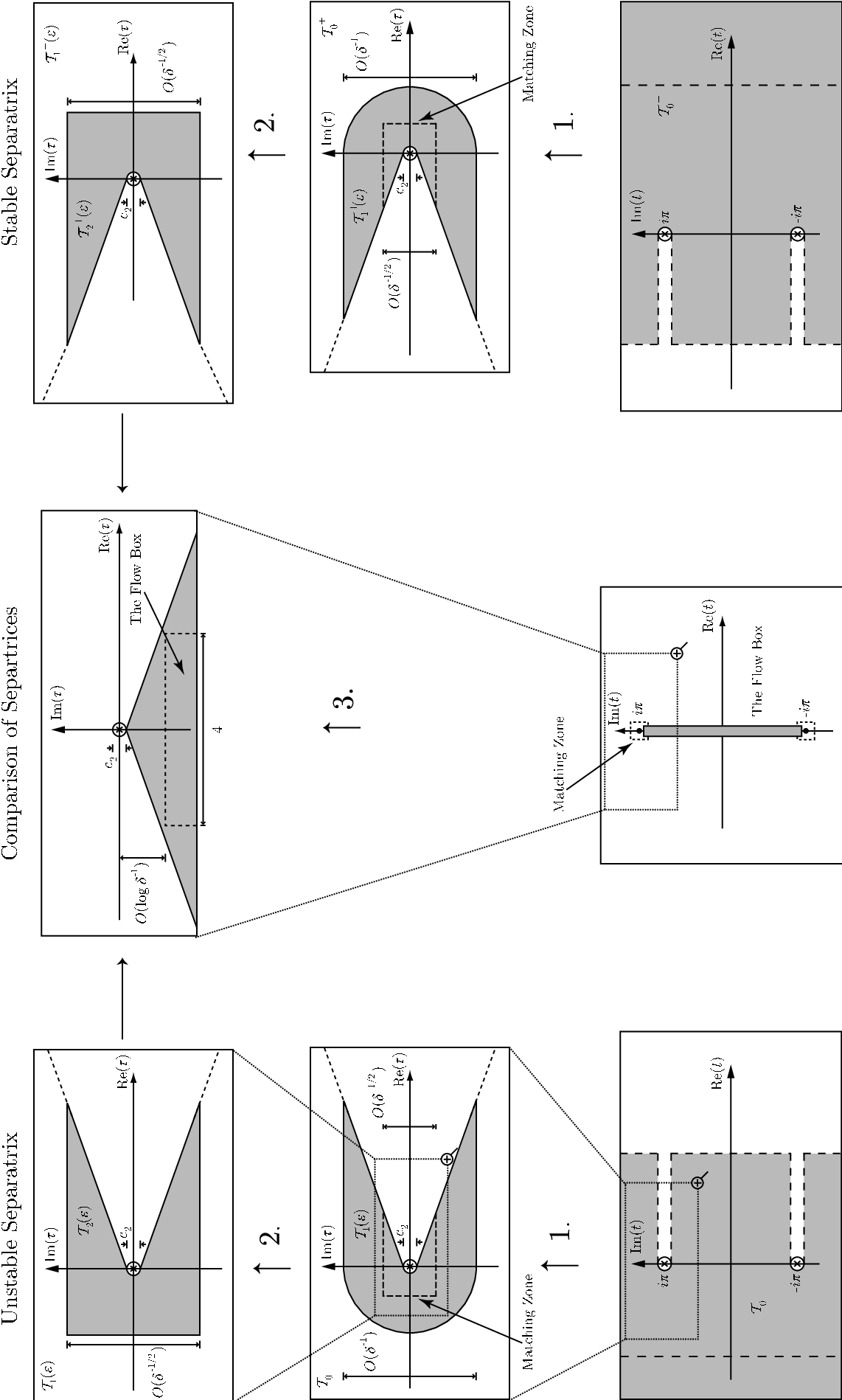
Figure 2: Overview of the proof: Domains of approximation

2 Overview of the proof

In this section we will describe the main steps of the proof postponing proofs of technical statements to subsequent sections. Before proceeding to the proof we need to introduce some definitions.

In this paper we will use power series in x,yx,y and ε\varepsilon. The arguments are easier when terms of a similar magnitude are grouped together. We consider xx to be of order 2, yy to be of order 3 and ε\varepsilon of order 44. We say that a polynomial QpQ_{p} is quasi-homogeneous of order pp if it satisfies the identity

Qp​(λ2​x,λ3​y,λ4​ε)=λp​Qp​(x,y,ε).Q_{p}(\lambda^{2}x,\lambda^{3}y,\lambda^{4}\varepsilon)=\lambda^{p}Q_{p}(x,y,\varepsilon)\,. (2.1)

Any power series can be represented as a sum of quasi-homogeneous polynomials.

In order to shorten the notation, we define

O^n:=O⁡((max⁡{|x|1/2,|y|1/3,ε1/4})n)\hat{O}_{n}:=O\left(\left(\max\{\,|x|^{1/2},|y|^{1/3},\varepsilon^{1/4}\,\}\right)^{n}\right)

and write O^n,n+1\hat{O}_{n,n+1} for a vector with components (O^n,O^n+1)(\hat{O}_{n},\hat{O}_{n+1}). It is easy to see that Qp=O^pQ_{p}=\hat{O}_{p}.

2.1 Standard scaling and limit flow

The change of the variables

x=δ2​X,y=δ3​Y,ε=δ4x=\delta^{2}X,\quad y=\delta^{3}Y,\quad\varepsilon=\delta^{4} (2.2)

is called the standard scaling. In the new variables the map fεf_{\varepsilon} takes the form of a close to identity map

Fδ=id+δ​Gδ.F_{\delta}=\mathrm{id}+\delta G_{\delta}. (2.3)

We note that G0G_{0} is called the limit flow. Its time-δ\delta map ΦG0δ=id+δ​G0+O⁡(δ2)\Phi_{G_{0}}^{\delta}=\mathrm{id}+\delta G_{0}+O(\delta^{2}) and therefore is O⁡(δ2)O(\delta^{2}) close to FδF_{\delta}.

Taking into account that f0​(0)=0f_{0}(0)=0 and the equality (1.1) we obtain

G0=(Y−a​X2+b)G_{0}=\left(\begin{array}[]{c}Y\\ -aX^{2}+b\end{array}\right)

for some constants a,ba,b. The same constants enter the non-degeneracy assumption (1.3). Indeed, the limit flow is Hamiltonian with the Hamilton function

H0=Y22+a​X33−b​XH_{0}=\frac{Y^{2}}{2}+\frac{aX^{3}}{3}-bX

which coincides, after reverting the standard scaling and scaling time, with (1.2). The dynamics of the limit flow is defined by the system of Hamiltonian equations:

X˙=Y,Y˙=−a​X2+b.\dot{X}=Y,\qquad\dot{Y}=-aX^{2}+b.

The limit flow has a saddle equilibrium at (−ba,0)(-\sqrt{\frac{b}{a}},0). At this point the linearised vector-field has a positive eigenvalue μ0=4​a​b4\mu_{0}=\sqrt[4]{4ab}. The separatrix of the limit flow can be found explicitly by integrating the Hamiltonian equations:

X0​(t)=−ba+3​a​bcosh2⁡μ0​t2,Y0​(t)=−3​a​b​μ0​sinh⁡μ0​t2cosh3⁡μ0​t2.X_{0}(t)=-\sqrt{\frac{b}{a}}+\frac{3\sqrt{ab}}{\cosh^{2}\frac{\mu_{0}t}{2}},\qquad Y_{0}(t)=-3\sqrt{ab}\mu_{0}\frac{\sinh\frac{\mu_{0}t}{2}}{\cosh^{3}\frac{\mu_{0}t}{2}}\,.

A substitution shows that these functions satisfy the Hamiltonian system. Obviously they converge to the saddle equilibrium as t→±∞t\to\pm\infty.

It is convenient to scale time and define the separatrix solution of the limit flow by

φ0​(t)=(X0,Y0)​(t/μ0).\varphi_{0}(t)=(X_{0},Y_{0})(t/\mu_{0})\,. (2.4)

This function satisfies the differential equation

φ˙0=μ0−1J∇H0(φ0).\dot{\varphi}_{0}=\mu_{0}^{-1}\mathrm{J}\nabla H_{0}(\varphi_{0})\,.

We will consider the separatrix solution for complex values of tt. We note that φ0\varphi_{0} is analytic for all complex tt except for second order poles at i​π​(2​k+1)i\pi(2k+1) with k∈ℤk\in\mathbb{Z}. In particular this solution is analytic in the strip |Im(t)|<π|\mathop{\rm Im}(t)|<\pi and has poles at the points t∗=±π​it_{*}=\pm\pi i on its boundary. These singularities play the central role in our analysis.

2.2 Formal interpolation and Formal separatrix

We use hεn=∑p=6n+5hp​(x,y,ε)h_{\varepsilon}^{n}=\sum_{p=6}^{n+5}h_{p}(x,y,\varepsilon) to denote a partial sum of a formal series

hε=∑p≥6hp​(x,y,ε)h_{\varepsilon}=\sum_{p\geq 6}h_{p}(x,y,\varepsilon) (2.5)

where hp​(x,y,ε)h_{p}(x,y,\varepsilon) are quasi-homogeneous polynomials of order pp. In Section 3.2 we will prove that there exists a unique formal series such that for each n∈ℕn\in\mathbb{N}

fε=Φhεn1+O^n+3,n+4,f_{\varepsilon}=\Phi_{h_{\varepsilon}^{n}}^{1}+\hat{O}_{n+3,n+4}\,, (2.6)

where Φhεn1\Phi_{h_{\varepsilon}^{n}}^{1} is the time one map with hamiltonian hεnh_{\varepsilon}^{n}. The leading order of the series is given by (1.2). It is a quasi-homogeneous polynomial of order 66 and coincides, up to scaling of the space and time variables, with the Hamiltonian of the limit flow.

We say that the series hεh_{\varepsilon} formally interpolates the map fεf_{\varepsilon}. We should not expect the series hεh_{\varepsilon} to converge.

Theorem 2.1 (Formal separatrix).

If hεh_{\varepsilon} is a formal Hamiltonian of the form (2.5) and its leading order satisfies the non-degeneracy condition (1.3), then there is a unique formal series

μ⁡(δ)=∑k≥0μk​δ2​k+1\mu(\delta)=\sum_{k\geq 0}\mu_{k}\delta^{2k+1}

such that the equation

μ(δ)𝐗˙=J∇hε(𝐗)\mu(\delta)\dot{\mathbf{X}}=\mathrm{J}\nabla h_{\varepsilon}(\mathbf{X}) (2.7)

has a formal solution of the form

𝐗⁡(t,ε)=(∑p≥1δ2​p​Xp1+η˙0​∑p≥1δ2​p+1​Xp−12η˙0​∑p≥1δ2​p+1​Yp−12+∑p≥2δ2​p​Yp1)\mathbf{X}(t,\varepsilon)=\left(\begin{array}[]{c}\sum\limits_{p\geq 1}\delta^{2p}X_{p}^{1}+\dot{\eta}_{0}\sum\limits_{p\geq 1}\delta^{2p+1}X_{p-1}^{2}\\ \dot{\eta}_{0}\sum\limits_{p\geq 1}\delta^{2p+1}Y_{p-1}^{2}+\sum\limits_{p\geq 2}\delta^{2p}Y_{p}^{1}\end{array}\right) (2.8)

where Xp1,Yp1,Xp2,Yp2X_{p}^{1},Y_{p}^{1},X_{p}^{2},Y_{p}^{2} are polynomials of order pp in η0=cosh−2⁡t2\eta_{0}=\cosh^{-2}\frac{t}{2}.

The proof of this theorem is placed in Section 4. We remind that δ=ε1/4\delta=\varepsilon^{1/4}.

We say that 𝐗\mathbf{X} is a formal separatrix. The series hεh_{\varepsilon} may diverge and consequently there is no reason to expect that the formal separatrix converges. On the other hand we will see that its partial sums provide a rather accurate approximation for the separatrices of the map fεf_{\varepsilon}.

Let us consider the domain

𝒯0={t∈ℂ:Re(t)≤r1 and φ0(t−s)∈𝒟,∀s≥0}\mathcal{T}_{0}=\left\{\;t\in\mathbb{C}\;:\;\mathop{\rm Re}(t)\leq r_{1}\ \mbox{ and }\ \varphi_{0}(t-s)\in\mathcal{D},\ \forall s\geq 0\;\right\} (2.9)

where r1>0r_{1}>0 is an arbitrary constant and 𝒟\mathcal{D} is a bounded domain. Later we will assume it to be a sufficiently large ball centred around the origin. Of course, some constants in future estimates will depend on the choice of r1r_{1} and 𝒟\mathcal{D}.

Lemma 2.2.

For any n∈ℕn\in\mathbb{N}, the Hamiltonian hδnh_{\delta}^{n} has a saddle equilibrium with a Lyapunov exponent μn,δ>0\mu_{n,\delta}>0 in a neighbourhood of the origin. Moreover, there exists a separatrix solution φδn\varphi_{\delta}^{n} of the equation

φ˙δn=μn,δ−1J∇hδn|φδn\dot{\varphi}_{\delta}^{n}=\mu_{n,\delta}^{-1}\left.\mathrm{J}\nabla h_{\delta}^{n}\right|_{\varphi_{\delta}^{n}} (2.10)

such that uniformly for t∈𝒯0t\in\mathcal{T}_{0}

φδn​(t)=𝐗n​(t,δ)+O⁡(δn),\varphi_{\delta}^{n}(t)=\mathbf{X}^{n}(t,\delta)+O(\delta^{n})\,,

where 𝐗n\mathbf{X}^{n} denotes the sum of the first nn orders in δ\delta of the formal series (2.8).

Proof.

The proof is straightforward: this lemma is a statement about polynomial vector fields and after the standard scaling the saddle of the equation is non-degenerate. ∎

Let 𝐗\mathbf{X} be the formal separatrix given by (2.8)\left(\ref{Sum_FormalSep}\right). We will study it close to the singularity by substituting t=i​π+τ​log⁡λδt=i\pi+\tau\log\lambda_{\delta} and expanding Xk1,2,Yk1,2X_{k}^{1,2},Y_{k}^{1,2} into their Laurent series. We also re-expand log⁡λδ=μ⁡(δ)\log\lambda_{\delta}=\mu(\delta). The result is a formal series of the form

𝐗=(∑m≥0δ2​m​τ2​m−2​∑k≥0xm​k​τ−k,∑m≥0δ2​m​τ2​m−3​∑k≥0ym​k​τ−k),\mathbf{X}=\left(\sum_{m\geq 0}\delta^{2m}\tau^{2m-2}\sum_{k\geq 0}x_{mk}\tau^{-k},\sum_{m\geq 0}\delta^{2m}\tau^{2m-3}\sum_{k\geq 0}y_{mk}\tau^{-k}\right), (2.11)

where xm​kx_{mk} and ym​ky_{mk} are real coefficients. See Section 4.3 for a derivation of (2.11). It is convenient to introduce formal power series in τ\tau by setting

ψ^m=(τ2​m−2​∑k≥0xm​k​τ−k,τ2​m−3​∑k≥0ym​k​τ−k)\hat{\psi}_{m}=\left(\tau^{2m-2}\sum_{k\geq 0}x_{mk}\tau^{-k},\tau^{2m-3}\sum_{k\geq 0}y_{mk}\tau^{-k}\right) (2.12)

for m≥0m\geq 0. Then

𝐗=∑m≥0δ2​m​ψ^m​(τ).\mathbf{X}=\sum_{m\geq 0}\delta^{2m}\hat{\psi}_{m}(\tau)\,. (2.13)

We will use these formal series in the complex matching procedure described in Section 2.6.

2.3 Separatrices for close-to-identity maps

Let us consider a family of close to identity maps (2.3). For the purpose of this section it is not necessary to assume that the map is obtained as a result of the standard scaling.

The implicit function theorem implies that if the limit flow G0G_{0} has a non-degenerate equilibrium then FδF_{\delta} has an analytic family of fixed points which tend to the equilibrium when δ→0\delta\rightarrow 0. If the equilibrium is a saddle then the fixed point of FδF_{\delta} is also a saddle (see Section 5.1 for formal statements and proofs).

The separatrix of FδF_{\delta} is close to the separatrix of the limit flow (see [9]). We will use a more accurate approximation provided by a separatrix of an (approximately) interpolating flow. Let us state it more formally.

Let 𝒟⊂ℂ2\mathcal{D}\subset\mathbb{C}^{2} be a bounded domain and assume the origin is inside 𝒟\mathcal{D}.

Theorem 2.3 (Approximation theorem).

Let FδF_{\delta} be an analytic family of area preserving maps such that the limit flow has a saddle equilibrium at the origin. Let HδnH_{\delta}^{n} be a Hamiltonian function such that

Fδ=ΦHδnδ+O⁡(δn+1)F_{\delta}=\Phi_{H_{\delta}^{n}}^{\delta}+O(\delta^{n+1}) (2.14)

on 𝒟\mathcal{D} and ϕδn\phi_{\delta}^{n} be a separatrix solution of the equation

ϕ˙δn=μn,δ−1J∇Hδn\dot{\phi}_{\delta}^{n}=\mu_{n,\delta}^{-1}\mathrm{J}\nabla H_{\delta}^{n}

such that

ϕδn​(t)=φ0​(t)+O⁡(δ)\phi_{\delta}^{n}(t)=\varphi_{0}(t)+O(\delta)

for all t∈𝒯0t\in\mathcal{T}_{0}. Then there exists a parametrisation Ψ−\Psi^{-} of the local unstable separatrix of the map FδF_{\delta} which satisfies the equation

Ψ−​(t+log⁡λδ)=Fδ​(Ψ−​(t))\Psi^{-}(t+\log\lambda_{\delta})=F_{\delta}(\Psi^{-}(t)) (2.15)

and

Ψ−​(t)=ϕδn​(t)+O⁡(δn)\Psi^{-}(t)=\phi_{\delta}^{n}(t)+O(\delta^{n}) (2.16)

uniformly on the set 𝒯0\mathcal{T}_{0}.

The proof of this theorem consists of two steps. First the theorem is proved for the local separatrix which corresponds to a half-plane Ret<−r0\mathop{\rm Re}t<-r_{0} as described in Section 5.3. Then an extension lemma (Lemma 5.3) stated and proved in Section 5.4 is applied.

For completeness, we also provide a proof of the existence for the Hamiltonian HδnH_{\delta}^{n} in Section 5.2.

2.4 Parametrisation the separatrices

We note that the existence of a parameterisation which satisfies equation (1.5) follows from the general theory [13]. The parametrization is not unique and is defined up to a translation t↦t+t0​(ε)t\mapsto t+t_{0}(\varepsilon). The next theorem states that there is a parameterisation which is close to the separatrix of the interpolating flow.

Let φδn\varphi_{\delta}^{n} be defined by Lemma 2.2.

Theorem 2.4 (Existence and Local approximation).

Equation (1.5) has a solution

ψ−​(t)=φδn​(t)+On+2,n+3​(δ)\psi^{-}(t)=\varphi_{\delta}^{n}(t)+O_{n+2,n+3}(\delta) (2.17)

uniformly for t∈𝒯0t\in\mathcal{T}_{0}.

Proof.

The theory of the previous section applies to the map FδF_{\delta} obtained after the standard scaling of the map fεf_{\varepsilon}. Let 𝒟\mathcal{D} be a large ball of a fixed radius. Since the map fεf_{\varepsilon} is defined in an ε\varepsilon independent neighbourhood of the origin, the domain of the scaled map FδF_{\delta} contains the ball 𝒟\mathcal{D} provided ε\varepsilon is sufficiently small.

The limit flow separatrix φ0\varphi_{0} is given explicitly by (2.4) and has poles at i​π​(2​k+1)i\pi(2k+1) for each k∈ℤk\in\mathbb{Z}. Therefore the set 𝒯0\mathcal{T}_{0} takes the shape similar to the one shown on Figure 3: it is a half plane Ret<r1\mathop{\rm Re}t<r_{1} without “shadows” of small disks centred around the singular points of φ0\varphi_{0}.

Refer to caption
Figure 3: Domain 𝒯0\mathcal{T}_{0}.

The interpolating Hamiltonian is obtained from (2.5) after the change of variables (2.2). Although the change of variables is not symplectic it has a constant Jacobian, and therefore the Hamiltonian flow of hδnh_{\delta}^{n} is transformed into a Hamiltonian flow with the Hamiltonian function

Hδn=∑k=1nδk​h5+k​(X,Y,1).H_{\delta}^{n}=\sum_{k=1}^{n}\delta^{k}h_{5+k}(X,Y,1). (2.18)

Indeed, under the standard scaling the symplectic form becomes d​x∧d​y=δ5​d​X∧d​Ydx\wedge dy=\delta^{5}dX\wedge dY, to work with the standard symplectic form in the scaled variables we scale the Hamiltonian by δ−5\delta^{-5}. The upper bound (2.14), which is necessary to apply Theorems 2.3, follows from (2.6) and (2.2).

To complete the proof we reverse the standard scaling which transforms the error term O⁡(δn)O(\delta^{n}) of equation (2.16) into On+2,n+3​(δ)O_{n+2,n+3}(\delta). ∎

2.5 Extension towards the singularity

The theory presented in the previous subsection provides a rather accurate approximation for the invariant manifolds. However, it is not sufficient to distinguish between the stable and unstable separatrices of the map FδF_{\delta}. Instead of further improving the accuracy, we will study the separatrices for values of tt closer to the singular points of the limit flow separatrix. In this region the splitting of the separatrices is larger and consequently easier to detect. This extension is sensitive to the form of the map and cannot be performed with the same level of generality as the estimates of Section 2.3. So from now on we restrict our consideration to our original map fεf_{\varepsilon}.

Let us fix two small positive constants c1c_{1} and β\beta, and consider a domain 𝒯1​(ε)\mathcal{T}_{1}(\varepsilon) shown on Figure 4 (left), which also depends on a constant c2>0c_{2}>0. The constant c2c_{2} is to be chosen sufficiently large to ensure that φ0\varphi_{0}, the separatrix of the limit flow written in the unscaled variables, does not leave a small ε\varepsilon-independent ball centred around the origin.

It is convenient to work with a time parameter centred at the singularity and to scale the time step to one, hence we let

τ=t−i​πlog⁡λδ.\tau=\frac{t-i\pi}{\log\lambda_{\delta}}. (2.19)

The domain 𝒯1​(ε)\mathcal{T}_{1}(\varepsilon) expressed in the terms of τ\tau is shown on Figure 4 (right).

Refer to caption
Refer to caption
Figure 4: An amplification of a neighbourhood of t=i​πt=i\pi shows the domain 𝒯1​(ε)\mathcal{T}_{1}(\varepsilon) in which the unstable separatrix is still reasonably well approximated by the separatrix of the limit flow (left). The same domain on the plane of τ\tau (right).
Theorem 2.5.

Let ψ−\psi^{-} be defined by Theorem 2.4. There is c2>0c_{2}>0 such that

ψ−​(τ)=φδn​(τ)+On,n+1​(τ−1)\psi^{-}(\tau)=\varphi_{\delta}^{n}(\tau)+O_{n,n+1}(\tau^{-1}) (2.20)

uniformly for all τ∈𝒯1​(ε)\tau\in\mathcal{T}_{1}(\varepsilon) and ε∈(0,ε0)\varepsilon\in(0,\varepsilon_{0}).

We note that t=i​π+τ​log⁡λδt=i\pi+\tau\log\lambda_{\delta} and we have overloaded notation by writing ψ−​(τ)\psi^{-}(\tau) instead of ψ−​(i​π+τ​log⁡λδ)=ψ−​(t)\psi^{-}(i\pi+\tau\log\lambda_{\delta})=\psi^{-}(t).

The estimate (2.20) is uniform which means that the constant in the term On,n+1​(τ−1)O_{n,n+1}(\tau^{-1}) is independent from both ε\varepsilon and τ\tau. It is important because the size of 𝒯1​(ε)\mathcal{T}_{1}(\varepsilon) increases as ε→0\varepsilon\to 0 and includes τ\tau up to the order of δ−1=ε−1/4\delta^{-1}=\varepsilon^{-1/4}. We note that in Theorem 2.5 the error of the approximation is of order O⁡(δn)O(\delta^{n}) on the left boundary of 𝒯1​(ε)\mathcal{T}_{1}(\varepsilon) but it is just of order O⁡(1)O(1) on the boundary near the central circle.

Therefore the theorem suggests that the distance between the separatrix of the map and separatrix of the interpolating flow may gradually increase as the parameter tt comes closer to i​πi\pi.

2.6 Complex matching

In this section we construct another approximation for ψ−\psi^{-} which provides higher accuracy in the central part of 𝒯1​(ε)\mathcal{T}_{1}(\varepsilon). Let us start by looking for a formal solution

ψ^​(τ)=∑k≥0δ2​k​ψk​(τ)\hat{\psi}(\tau)=\sum_{k\geq 0}\delta^{2k}\psi_{k}(\tau) (2.21)

of the separatrix equation

ψ^​(τ+1)=fε​(ψ^​(τ)).\hat{\psi}(\tau+1)=f_{\varepsilon}(\hat{\psi}(\tau)). (2.22)

We assume that the new time τ\tau is related to the original tt by (2.19). We formally substitute the series (2.21) into the equation (2.22) and expand the right hand side in powers of δ2\delta^{2}. Collecting terms of equal order in δ\delta we get at the leading order

ψ0​(τ+1)=f0​(ψ0​(τ)),\psi_{0}(\tau+1)=f_{0}(\psi_{0}(\tau)), (2.23)

and the following system of equations for all other orders:

ψ1​(τ+1)\displaystyle\psi_{1}(\tau+1) =\displaystyle= D​f0​(ψ0​(τ))​ψ1​(τ),\displaystyle Df_{0}(\psi_{0}(\tau))\psi_{1}(\tau),
ψ2​(τ+1)\displaystyle\psi_{2}(\tau+1) =\displaystyle= D​f0​(ψ0​(τ))​ψ2​(τ)+R2​(ψ0,ψ1),\displaystyle Df_{0}(\psi_{0}(\tau))\psi_{2}(\tau)+R_{2}(\psi_{0},\psi_{1}),

In general, the equation corresponding to δ2​m\delta^{2m} with m≥2m\geq 2 can be written as

ψm​(τ+1)=D​f0​(ψ0)​ψm​(τ)+Rm​(ψ0,ψ1,…,ψm−1),\psi_{m}(\tau+1)=Df_{0}(\psi_{0})\psi_{m}(\tau)+R_{m}(\psi_{0},\psi_{1},\ldots,\psi_{m-1}), (2.24)

where RmR_{m} is a polynomial in (ψ1,…,ψm−1)\left(\psi_{1},\ldots,\psi_{m-1}\right). We stress that the dependence on ψ0\psi_{0} is not necessarily polynomial. For example,

R2=ψ1t​D2​f0​(ψ0)​ψ1+f1​(ψ0)R_{2}=\psi_{1}^{t}D^{2}f_{0}(\psi_{0})\psi_{1}+f_{1}(\psi_{0})

where t is used to denote the transposition and f1f_{1} is a coefficient of the Taylor series fε=∑k≥0εk​fkf_{\varepsilon}=\sum_{k\geq 0}\varepsilon^{k}f_{k}.

An analytic solution ψm−\psi^{-}_{m} of the equation (2.24) can be selected by the following asymptotic condition:

ψm−(τ)≍ψ^m(τ) as τ→∞ in the sector β0<arg⁡τ<2​π−β0.\psi^{-}_{m}(\tau)\asymp\hat{\psi}_{m}(\tau)\qquad\mbox{ as $\tau\to\infty$ in the sector $\beta_{0}<\arg\tau<2\pi-\beta_{0}$}\,. (2.25)

The formal series ψ^m​(τ)\hat{\psi}_{m}(\tau) comes from the re-expansion of the formal separatrix given by (2.13). In fact, ψ^m\hat{\psi}_{m} is a formal solution of equation (2.24).

The method of fixing a solution in one region by initial or boundary conditions which come from a neighbouring region is known as “complex matching”.

Refer to caption

Figure 5: Complex matching.

We will now continue with the approximation inside the matching zone, we call this domain 𝒯2​(ε)\mathcal{T}_{2}(\varepsilon):

𝒯2(ε)={τ∈𝒯1(ε):Reτ>−δ1/2,−δ1/2<Imτ<δ1/2}.\mathcal{T}_{2}(\varepsilon)=\left\{\tau\in\mathcal{T}_{1}(\varepsilon):\mathop{\rm Re}\tau>-\delta^{1/2},\,-\delta^{1/2}<\mathop{\rm Im}\tau<\delta^{1/2}\right\}.
Refer to caption
Figure 6: Complex matching.
Theorem 2.6 (Second approximation theorem).
ψ−​(τ)=∑k=0n−1δ2​k​ψk−​(τ)+O⁡(δn)\psi^{-}(\tau)=\sum_{k=0}^{n-1}\delta^{2k}\psi_{k}^{-}(\tau)+O(\delta^{n})

uniformly in 𝒯2​(ε)\mathcal{T}_{2}(\varepsilon).

We note that this theorem implies the following.

Corollary 2.7.

There is a parametrisation of the unstable separatrix such that

ψ−​(τ)=∑k=0n−1δ2​k​ψk−​(τ)+O⁡((δ​τ)2​n).\psi^{-}(\tau)=\sum_{k=0}^{n-1}\delta^{2k}\psi_{k}^{-}(\tau)+O((\delta\tau)^{2n}). (2.26)

uniformly in 𝒯2​(ε)\mathcal{T}_{2}(\varepsilon).

Proof.

The asymptotic boundary conditions implies ψk−​(τ)=O⁡(τ2​k)\psi^{-}_{k}(\tau)=O(\tau^{2k}). Then the theorem with nn replaced by 2​n2n implies

ψ−​(τ)\displaystyle\psi^{-}(\tau) =\displaystyle= ∑k=02​n−1δ2​k​ψk−​(τ)+O⁡(δ2​n)\displaystyle\sum_{k=0}^{2n-1}\delta^{2k}\psi_{k}^{-}(\tau)+O(\delta^{2n})
=\displaystyle= ∑k=0n−1δ2​k​ψk−​(τ)+O⁡((δ​τ)2​n).\displaystyle\sum_{k=0}^{n-1}\delta^{2k}\psi_{k}^{-}(\tau)+O((\delta\tau)^{2n}).

∎

2.7 The stable manifold

So far we have only considered the unstable separatrix. In order to estimate the splitting of separatrices we also need to study the stable one. We note that the stable manifold is an unstable one for the inverse map.

Therefore the study of the stable separatrix is analogous to the study of the unstable one but with time reversed. The transformation t↦−tt\mapsto-t swaps the upper and lower half-planes of ℂ\mathbb{C} and it is convenient to use real-analytic symmetry to swap these back. Let 𝒯0+,𝒯1+​(ε),𝒯2+​(ε)⊂ℂ\mathcal{T}_{0}^{+},\mathcal{T}_{1}^{+}(\varepsilon),\mathcal{T}_{2}^{+}(\varepsilon)\subset\mathbb{C} denote domains obtained by reflecting 𝒯0,𝒯1​(ε),𝒯2​(ε)\mathcal{T}_{0},\mathcal{T}_{1}(\varepsilon),\mathcal{T}_{2}(\varepsilon) in the imaginary axis respectively. The limit flow and approximately interpolating flows are integrable and their stable and unstable separatrices coincide. Therefore the same separatrix solution arise and the same formal expansion (2.13) is used for the complex matching of the stable separatrix. However, the matching is done on the right hand side of the singularity with asymptotic boundary conditions as τ→+∞\tau\rightarrow+\infty.

Refer to caption
Figure 7: The shadowed region represents the domain of validity for the local approximation theorem for the stable separatrix.

Similarly to Theorem 2.4, we conclude that for every n∈ℕn\in\mathbb{N} there is a solution ψ+\psi^{+} of the equation (1.5) such that

ψ+​(t)=φδ2​n​(t)+O2​n+2,2​n+3​(δ)\psi^{+}(t)=\varphi_{\delta}^{2n}(t)+O_{2n+2,2n+3}(\delta) (2.27)

uniformly for t∈𝒯0+t\in\mathcal{T}_{0}^{+} (see Figure 7). Note that we directly started with nn replaced by 2​n2n. For this solution, instead of (2.20) we get

ψ+​(t)=φδ2​n​(t)+O2​n,2​n+1​(τ−1)\psi^{+}(t)=\varphi_{\delta}^{2n}(t)+O_{2n,2n+1}(\tau^{-1}) (2.28)

uniformly in 𝒯1+​(ε)\mathcal{T}_{1}^{+}(\varepsilon) and ε∈(0,ε0)\varepsilon\in(0,\varepsilon_{0}) and instead of Corollary 2.7 we get

Corollary 2.8.

Uniformly in 𝒯2+​(ε)\mathcal{T}_{2}^{+}(\varepsilon)

ψ+​(τ)=∑k=0n−1δ2​k​ψk+​(τ)+O⁡((δ​τ)2​n)\psi^{+}(\tau)=\sum_{k=0}^{n-1}\delta^{2k}\psi^{+}_{k}(\tau)+O((\delta\tau)^{2n}) (2.29)

where ψk+​(τ)\psi_{k}^{+}(\tau) is the solution of the asymptotic boundary condition problem (2.23) or (2.24) subject to the asymptotic boundary conditions

ψk+(τ)≍ψ^k(τ) as τ→∞ in the sector −π+β0<arg⁡τ<π−β0.\psi^{+}_{k}(\tau)\asymp\hat{\psi}_{k}(\tau)\qquad\mbox{ as $\tau\to\infty$ in the sector $-\pi+\beta_{0}<\arg\tau<\pi-\beta_{0}$}\,.

We note that in general ψ0+≠ψ0−\psi_{0}^{+}\neq\psi_{0}^{-} [11, 14].

2.8 Upper bounds for the splitting of separatrices

We assume that both ψ−\psi^{-} and ψ+\psi^{+} are chosen to be closed to φδ2​n\varphi^{2n}_{\delta}. Then comparing the estimates (2.17) and (2.27)

ψ−​(t)−ψ+​(t)=O⁡(δ2​n)\psi^{-}(t)-\psi^{+}(t)=O(\delta^{2n})

uniformly in 𝒯0∩𝒯0+\mathcal{T}_{0}\cap\mathcal{T}_{0}^{+}. Then we use the estimates (2.28) (with nn replaced by 2​n2n) and (2.28) to conclude

ψ−​(t)−ψ+​(t)=O2​n,2​n+1​(τ−1)\psi^{-}(t)-\psi^{+}(t)=O_{2n,2n+1}(\tau^{-1})

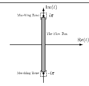
uniformly in 𝒯1​(ε)∩𝒯1+​(ε)\mathcal{T}_{1}(\varepsilon)\cap\mathcal{T}^{+}_{1}(\varepsilon). Taking into account the difinitions of the domains we see that the union of validity domains of these two estimates includes the rectangle defined by the inequalities |Imt|<π−δ1/2|\mathop{\rm Im}{t}|<\pi-\delta^{1/2} and |Ret|<δ1/2|\mathop{\rm Re}{t}|<\delta^{1/2} and for these values of tt

ψ+​(t)−ψ−​(t)=O⁡(τ−n)=O⁡(δn).\psi^{+}(t)-\psi^{-}(t)=O(\tau^{-n})=O(\delta^{n})\,. (2.30)

In the innermost region 𝒯2​(ε)\mathcal{T}_{2}(\varepsilon), closer to the singularity at i​πi\pi, we use a different argument. In this region the estimate has to be be close to optimal: we will use the upper bound to show that the square of the distance between the stable and unstable separatrices is negligible compared to the leading term of the splitting (on a line with Imτ=−σ​log⁡δ\mathop{\rm Im}\tau=-\sigma\log\delta).

The upper bound for the splitting near the singularity is obtained in the following way: by Corollaries 2.7 and 2.8

ψ+​(τ)−ψ−​(τ)=∑k=0n−1δ2​k​(ψk+​(τ)−ψk−​(τ))+O⁡((δ​τ)2​n)\psi^{+}(\tau)-\psi^{-}(\tau)=\sum_{k=0}^{n-1}\delta^{2k}\left(\psi_{k}^{+}(\tau)-\psi_{k}^{-}(\tau)\right)+O\left((\delta\tau)^{2n}\right) (2.31)

uniformly in 𝒯2​(ε)∩𝒯2+​(ε)\mathcal{T}_{2}(\varepsilon)\cap\mathcal{T}_{2}^{+}(\varepsilon). We use that

ψk+​(τ)−ψk−​(τ)=O⁡(τmk​e−2​π​i​τ)\psi_{k}^{+}(\tau)-\psi_{k}^{-}(\tau)=O(\tau^{m_{k}}e^{-2\pi i\tau}) (2.32)

provided −π+β<arg⁡τ<−β-\pi+\beta<\arg\tau<-\beta and Imτ<−c2\mathop{\rm Im}\tau<-c_{2}.Consequently

ψ+​(τ)−ψ−​(τ)=O⁡(τ4​e−2​π​i​τ)+O⁡((δ​τ)2​n)\psi^{+}(\tau)-\psi^{-}(\tau)=O(\tau^{4}e^{-2\pi i\tau})+O((\delta\tau)^{2n}) (2.33)

provided −c2>Imτ>−δ−1/2-c_{2}>\mathop{\rm Im}\tau>-\delta^{-1/2} and −π+β<arg⁡τ<−β-\pi+\beta<\arg\tau<-\beta.

2.9 The flow box

In order to provide a quantitative description for the difference between ψ+\psi^{+} and ψ−\psi^{-} we use the method based on flow box coordinates. We will prove a theorem which essentially says that the restriction of the map fεf_{\varepsilon} on a non-invariant subset can be analytically interpolated by an autonomous Hamiltonian flow with one degree of freedom. The subset in question contains large (but again non-invariant) segments of the stable and unstable separatrices. Simultaneously we introduce “energy-time” coordinates (T,E)(T,E) for the interpolating flow.

Consider a domain in ℂ2\mathbb{C}^{2} defined by

𝒰δ=𝒯×ℰ={|Re(T)|<2,|Im(T)|<πlog⁡λδ−c3}×{|E|<E0(δ)}.\mathcal{U}_{\delta}=\mathcal{T}\times\mathcal{E}=\left\{\,\left|\mathop{\rm Re}(T)\right|<2,\ \left|\mathop{\rm Im}(T)\right|<\frac{\pi}{\log\lambda_{\delta}}-c_{3}\,\right\}\times\left\{\,\left|E\right|<E_{0}(\delta)\,\right\}. (2.34)
Refer to caption
Figure 8: Time component of the flow box coordinates (t:=T​log⁡λδt:=T\log\lambda_{\delta}).
Theorem 2.9 (The flow box theorem).

If c3c_{3} is sufficiently large, there exists a symplectic diffeomorphism S:𝒰δ→𝒱δ:=S⁡(𝒰δ)S:\mathcal{U}_{\delta}\to\mathcal{V}_{\delta}:=S(\mathcal{U}_{\delta}) such that

  1. 1.

    fε|𝒱δ=ΦE1\left.f_{\varepsilon}\right|_{\mathcal{V}_{\delta}}=\Phi_{E}^{1}, where E:𝒱δ→ℂE:\mathcal{V}_{\delta}\to\mathbb{C} is the second component of the map S−1S^{-1}.

  2. 2.

    S⁡(T,0)=ψ−​(T​log⁡λδ)S(T,0)=\psi^{-}(T\log\lambda_{\delta}) (Normalisation).

  3. 3.

    ‖S−1‖C2\left\|S^{-1}\right\|_{C^{2}} is bounded uniformly for ε∈(0,ε0)\varepsilon\in(0,\varepsilon_{0}).

It is convenient to consider S−1S^{-1} as a symplectic coordinate map defined on 𝒱δ\mathcal{V}_{\delta}. In coordinates (T,E)(T,E), the Hamiltonian equations with the Hamiltonian function EE take the form

T′=1,E′=0T^{\prime}=1\,,\qquad E^{\prime}=0

and can be easily integrated. The corresponding time-one map has the form (T,E)↦(T+1,E)(T,E)\mapsto(T+1,E). It coincides with S−1∘ΦE1∘SS^{-1}\circ\Phi^{1}_{E}\circ S. In the original coordinates the map ΦE1=fε\Phi_{E}^{1}=f_{\varepsilon}. Consequently the first property of SS means that SS conjugates fεf_{\varepsilon} and the translation:

(T+1,E)=S−1∘fε∘S⁡(T,E).(T+1,E)=S^{-1}\circ f_{\varepsilon}\circ S(T,E). (2.35)

Let us use (T⁡(x,y),E⁡(x,y))(T(x,y),E(x,y)) for the components of S−1S^{-1} and (x⁡(T,E),y⁡(T,E))(x(T,E),y(T,E)) for the components of SS. Equation (2.35) implies

T∘fε​(x,y)\displaystyle T\circ f_{\varepsilon}(x,y) =\displaystyle= T⁡(x,y)+1,\displaystyle T(x,y)+1\,, (2.36)
E∘fε​(x,y)\displaystyle E\circ f_{\varepsilon}(x,y) =\displaystyle= E⁡(x,y).\displaystyle E(x,y)\,. (2.37)

By the inverse function theorem, the Jacobian matrix D​S−1=(D​S)−1DS^{-1}=(DS)^{-1}. In coordinate form this equality implies that

(∂T∂x∂T∂y∂E∂x∂E∂y)=(∂x∂T∂x∂E∂y∂T∂y∂E)−1=(∂y∂E−∂x∂E−∂y∂T∂x∂T),\left(\begin{array}[]{cc}\frac{\partial T}{\partial x}&\frac{\partial T}{\partial y}\\[6.0pt] \frac{\partial E}{\partial x}&\frac{\partial E}{\partial y}\end{array}\right)=\left(\begin{array}[]{cc}\frac{\partial x}{\partial T}&\frac{\partial x}{\partial E}\\[6.0pt] \frac{\partial y}{\partial T}&\frac{\partial y}{\partial E}\end{array}\right)^{-1}=\left(\begin{array}[]{cc}\frac{\partial y}{\partial E}&-\frac{\partial x}{\partial E}\\[6.0pt] -\frac{\partial y}{\partial T}&\frac{\partial x}{\partial T}\end{array}\right),

where we used that the Jacobian matrix has the unit determinant to get the second equality. The second row gives the following Hamiltonian equations:

∂y∂T=−∂E∂xand∂x∂T=∂E∂y.\frac{\partial y}{\partial T}=-\frac{\partial E}{\partial x}\qquad\mbox{and}\qquad\frac{\partial x}{\partial T}=\frac{\partial E}{\partial y}\,.

Substituting E=0E=0 into the equations, using the normalisation condition in the form

(x⁡(T,0),y⁡(T,0))=ψ−​(T​log​λδ)=(ψ1−​(T​log​λδ),ψ2−​(T​log​λδ))\left(x(T,0),y(T,0)\right)=\psi^{-}(T\log\lambda_{\delta})=(\psi_{1}^{-}(T\log\lambda_{\delta}),\psi_{2}^{-}(T\log\lambda_{\delta}))

and switching to derivation with respect to tt (where t=T​log⁡λδt=T\log\lambda_{\delta}) we get

∂E∂x|ψ−\displaystyle\left.\frac{\partial E}{\partial x}\right|_{\psi^{-}} =\displaystyle= −log⁡λδ​ψ˙2−,\displaystyle-\log\lambda_{\delta}\,\dot{\psi}_{2}^{-}\,,
∂E∂y|ψ−\displaystyle\left.\frac{\partial E}{\partial y}\right|_{\psi^{-}} =\displaystyle= log⁡λδ​ψ˙1−.\displaystyle\log\lambda_{\delta}\,\dot{\psi}_{1}^{-}\,.

The last equation has the form of a Hamiltonian system with the Hamiltonian E⁡(x,y)E(x,y) after a time rescaling. For future reference we write this identity using the vector notation:

∇E​(ψ−)=−log⁡λδ​J​ψ˙−\nabla E(\psi^{-})=-\log\lambda_{\delta}\,{\mathrm{J}}\dot{\psi}^{-} (2.38)

where J=(01−10){\mathrm{J}}=\left(\begin{array}[]{rr}0&1\\ -1&0\end{array}\right) is the standard symplectic matrix.

Remark 2.10.

The following facts are not directly used in the proof. It is easy to see that equation (2.35) alone does not define SS uniquely. Indeed, consider a substitution (T,E)↦(T~,E~)(T,E)\mapsto(\widetilde{T},\widetilde{E}) of the form

(T~,E~)=(T+a⁡(T,E),b⁡(T,E))(\widetilde{T},\widetilde{E})=(T+a(T,E),b(T,E))

where aa and bb are 11-periodic in TT. A map S~\tilde{S} obtained as a result of this substitution also satisfy (2.35). Although the uniqueness is not important for our study, we note that the substitutions of this form exhaustively describe the freedom in the definition of SS.

The normalisation property of Theorem 2.9 does not eliminate this freedom completely but only fixes SS on the line E=0E=0 in a way which makes comparison between the stable and unstable separatrices more convenient.

2.10 Splitting function

Let us define the splitting function by11 1 The domain of this function is to be studied.

Θ⁡(T)=E∘ψ+​(T​log⁡λδ).\Theta(T)=E\circ\psi^{+}(T\log\lambda_{\delta}). (2.39)

We can use Θ\Theta to

  1. 1.

    Find the homoclinic points.

  2. 2.

    Find the homoclinic invariant ω\omega.

  3. 3.

    Calculate the lobe areas.

  4. 4.

    Calculate the distances between ψ+\psi^{+} and ψ−\psi^{-}.

Since E=0E=0 corresponds to the unstable separatrix, zeroes of the splitting functions correspond to homoclinic points, i.e., if Θ⁡(T1)=0\Theta(T_{1})=0 for some T1T_{1} then ψ+​(t1)∈W−\psi^{+}(t_{1})\in W^{-} for t1=T1​log⁡λt_{1}=T_{1}\log\lambda. Therefore there is t2t_{2} such that ψ+​(t1)=ψ−​(t2)\psi^{+}(t_{1})=\psi^{-}(t_{2}).

Let us consider the derivative of the splitting function with respect to TT at T=T1T=T_{1}:

d​Θd​T(T1)=∇Et|ψ+​(t1)d​ψ+d​T(T1logλ)=logλ∇Et|ψ−​(t2)ψ˙+(t1),\frac{d\Theta}{dT}(T_{1})=\left.\nabla E^{t}\right|_{\psi^{+}(t_{1})}\frac{d\psi^{+}}{dT}(T_{1}\log\lambda)=\log\lambda\,\left.\nabla E^{t}\right|_{\psi^{-}(t_{2})}\dot{\psi}^{+}(t_{1})\,,

where we used the equality ψ+​(t1)=ψ−​(t2)\psi^{+}(t_{1})=\psi^{-}(t_{2}). We use (2.38) to eliminate the gradient of EE:

d​Θd​T​(T1)=−log2⁡λ​(J​ψ˙−)t​ψ˙+=log2⁡λ​(ψ˙−)t​J​ψ˙+\frac{d\Theta}{dT}(T_{1})=-\log^{2}\!\lambda\,({\mathrm{J}}\dot{\psi}^{-})^{t}\dot{\psi}^{+}=\log^{2}\!\lambda\,(\dot{\psi}^{-})^{t}{\mathrm{J}}\dot{\psi}^{+}

since Jt=−J\mathrm{J}^{t}=-\mathrm{J}. Taking into account the definition of the symplectic form we get

d​Θd​T​(T1)=−log2⁡λ​Ω​(ψ˙−,ψ˙+).\frac{d\Theta}{dT}(T_{1})=-\log^{2}\!\lambda\,\Omega\left(\dot{\psi}^{-},\dot{\psi}^{+}\right).

We remind ourselves that the homoclinic invariant, also known as the Lazutkin invariant, is defined by

ω=Ω⁡(ψ˙+,ψ˙−).\omega=\Omega(\dot{\psi}^{+},\dot{\psi}^{-}).

Therefore we have established that the homoclinic invariant is proportional to the gradient of the splitting function

ω=1log2⁡λ​Θ′​(T1)\omega=\frac{1}{\log^{2}\lambda}\;\Theta^{\prime}(T_{1}) (2.40)

at its zero, Θ⁡(T1)=0\Theta(T_{1})=0.

Next, we note that Θ⁡(T)\Theta(T) is periodic. Indeed using the definition (2.39), equation (1.5) with t=T​log⁡λt=T\log\lambda and the equality (2.37) we obtain

Θ⁡(T+1)\displaystyle\Theta(T+1) =\displaystyle= E∘ψ+​((T+1)​log⁡λ)=E∘fε∘ψ+​(T​log⁡λ)\displaystyle E\circ\psi^{+}(\left(T+1\right)\log\lambda)=E\circ f_{\varepsilon}\circ\psi^{+}(T\log\lambda)
=\displaystyle= E∘ψ+​(T​log⁡λ)=Θ⁡(T).\displaystyle E\circ\psi^{+}(T\log\lambda)=\Theta(T)\,.

Hence we can write the Fourier series

Θ⁡(T)=∑k∈ℤΘk​e2​π​i​k​T.\Theta(T)=\sum_{k\in\mathbb{Z}}\Theta_{k}e^{2\pi ikT}.
Lemma 2.11.

Let c1>0c_{1}>0 be fixed and let ρ=π−c1\rho=\pi-c_{1}. If δ\delta is sufficiently small, the domain of the function Θ\Theta contains the strip

{T:|ImT|≤ρ/log⁡λδ}.\{\,T:|\mathop{\rm Im}T|\leq\rho/\log\lambda_{\delta}\,\}\,.

Moreover, for all s∈ℝs\in\mathbb{R}

Θ(s)=Θ1e2​π​i​s+Θ1∗e−2​π​i​s+O(e−4πρ/logλδ)\Theta(s)=\Theta_{1}e^{2\pi is}+\Theta_{1}^{*}e^{-2\pi is}+O(e^{-4\pi\rho/\log\lambda_{\delta}}) (2.41)

where Θ1≡Θ1​(δ)\Theta_{1}\equiv\Theta_{1}(\delta) is a first Fourier coefficient of Θ\Theta. The asymptotic formula (2.41) can be differentiated with respect to ss, the error term does not change its order.

Proof.

We note that on the strip the absolute value of Θ⁡(T)\Theta(T) does not exceed E0​(δ)E_{0}(\delta) defined in (2.34). Writing the classical integrals for Fourier coefficients of a periodic function and shifting the integration path to the boundary of the analyticity strip, we derive

|Θk|≤E0​(δ)​e−|k|​2​π​ρlog⁡λδ.\left|\Theta_{k}\right|\leq E_{0}(\delta)\mathrm{e}^{-\left|k\right|\frac{2\pi\rho}{\log\lambda_{\delta}}}. (2.42)

Since log⁡λδ\log\lambda_{\delta} is of the order of δ\delta all Fourier coefficients are exponentially small (the zero order coefficient being an exception). Moreover, the coefficients with |k|≥2|k|\geq 2 are negligible compared to the size of the separatrix splitting we intend to detect.

Now we show that Θ0\Theta_{0} is also negligible. We define an auxiliary function g⁡(s)=T∘ψ+​(s​log⁡λ)g(s)=T\circ\psi^{+}(s\log\lambda) which describes the TT component of the stable separatrix in the flow box coordinates. Using the definition (2.39), equation (1.5) with t=T​log⁡λt=T\log\lambda and the equality (2.36) we obtain

g⁡(s+1)\displaystyle g(s+1) =\displaystyle= T∘ψ+​((s+1)​log⁡λδ)=T∘fε∘ψ+​(s​log⁡λδ)\displaystyle T\circ\psi^{+}((s+1)\log\lambda_{\delta})=T\circ f_{\varepsilon}\circ\psi^{+}(s\log\lambda_{\delta})
=\displaystyle= T∘ψ+​(s​log⁡λδ)+1=g⁡(s)+1.\displaystyle T\circ\psi^{+}(s\log\lambda_{\delta})+1=g(s)+1.

Consequently g′g^{\prime} is periodic and its mean value is 1

∫T1T1+1(1−g′​(s))​𝑑s=0\int_{T_{1}}^{T_{1}+1}(1-g^{\prime}(s))ds=0 (2.43)

for any T1T_{1} from its domain.

Let T1T_{1} be a zero of the function Θ\Theta. Then 𝐩1=ψ+​(t1)=ψ−​(t2)\mathbf{p}_{1}=\psi^{+}(t_{1})=\psi^{-}(t_{2}) is an homoclinic point. The segments of the stable and unstable separatrices with their ends at 𝐩1\mathbf{p}_{1} and fε​(𝐩1)f_{\varepsilon}(\mathbf{p}_{1}) form a closed loop on the plane. The total algebraic area of this loop vanishes. Since SS is symplectic, this area can be evaluated in the flow box coordinates. The segment of the unstable separatrix is a straight line which connects the points (T2,0)(T_{2},0) and (T2+1,0)(T_{2}+1,0) and therefore the area is given by the integral

∫T1T1+1Θ⁡(s)​g′​(s)​𝑑s=∫T1T1+1Θ⁡(s)​𝑑g​(s)=0.\int_{T_{1}}^{T_{1}+1}\Theta(s)g^{\prime}(s)ds=\int_{T_{1}}^{T_{1}+1}\Theta(s)dg(s)=0. (2.44)
Refer to caption
Figure 9: Unstable separatrix is the ”x-axis” and the Stable one is a graph over it; The area is zero since the map is area-preserving.

Now we can come back to estimates for the zero order Fourier coefficient of the function Θ\Theta which is given by the integral

Θ0=∫T1T1+1Θ⁡(s)​𝑑s.\Theta_{0}=\int_{T_{1}}^{T_{1}+1}\Theta(s)ds\,.

Taking into account (2.44) we rewrite it

Θ0=∫T1T1+1Θ⁡(s)​(1−g′​(s))​𝑑s.\Theta_{0}=\int_{T_{1}}^{T_{1}+1}\Theta(s)(1-g^{\prime}(s))ds\,.

Then using equation (2.43) and the fact that Θ0\Theta_{0} is constant we get:

Θ0=∫T1T1+1(Θ⁡(s)−Θ0)​(1−g′​(s))​𝑑s.\Theta_{0}=\int_{T_{1}}^{T_{1}+1}(\Theta(s)-\Theta_{0})(1-g^{\prime}(s))ds\,.

Under the integral we see the product of two functions, each one is periodic and of zero mean. The Fourier series arguments show that

Θ(s)−Θ0=O(e−2πρ/logλδ)and1−g′(s)=O(e−2πρ/logλδ)\Theta(s)-\Theta_{0}=O(e^{-2\pi\rho/\log\lambda_{\delta}})\qquad\mbox{and}\qquad 1-g^{\prime}(s)=O(e^{-2\pi\rho/\log\lambda_{\delta}}) (2.45)

since ss is real. Consequently, Θ0\Theta_{0} is extremely small:

Θ0=O(e−4πρ/logλδ),\Theta_{0}=O(e^{-4\pi\rho/\log\lambda_{\delta}}),

as the exponent in the right hand side is almost double the expected leading order of the separatrices splitting.

In particular, combining the last upper bound with (2.42) we conclude that on the real axis

|Θ(s)|≤∑k∈ℤ|Θk|=O(e−2πρ/logλδ).|\Theta(s)|\leq\sum_{k\in\mathbb{Z}}|\Theta_{k}|=O(e^{-2\pi\rho/\log\lambda_{\delta}})\,. (2.46)

Moreover, this function is almost sinusoidal since if we keep apart the two largest Fourier coefficients the sum of all others is very small and for s∈ℝs\in\mathbb{R} we get (2.41).

Of course the Fourier coefficients Θ1\Theta_{1} and Θ−1=Θ1∗\Theta_{-1}=\Theta_{1}^{\ast} depend on δ\delta and are exponentially small due to the upper bound (2.42) with |k|=1|k|=1. Nevertheless the the error term is much smaller than the upper bound for Θ±1\Theta_{\pm 1}. In the next section we will construct an asymptotic expansion for Θ−1\Theta_{-1} and conclude that generically it really dominates the error. ∎

Finally we show how to use the splitting function to estimate the lobe area between the stable and unstable manifolds. Suppose T1T_{1} and T2T_{2} are two zeroes of Θ\Theta. Then the lobe area is represented by the following integral:

∫T1T2Θ⁡(s)​g′​(s)​𝑑s=∫T1T2Θ⁡(s)​𝑑s+∫T1T2Θ⁡(s)​(g′​(s)−1)​𝑑s.\int_{T_{1}}^{T_{2}}\Theta(s)g^{\prime}(s)ds=\int_{T_{1}}^{T_{2}}\Theta(s)ds+\int_{T_{1}}^{T_{2}}\Theta(s)(g^{\prime}(s)-1)ds\,.

Taking into account the upper bound (2.45) and (2.46) for the functions under the second integral we conclude that the lobe area equals to

∫T1T2Θ(s)ds+O(e−4πρ/logλδ).\int_{T_{1}}^{T_{2}}\Theta(s)ds+O(e^{-4\pi\rho/\log\lambda_{\delta}})\,.

2.11 Asymptotic expansion for the homoclinic invariant

Refer to caption
Figure 10: Domain used to estimate the first Fourier coefficient of the splitting function

Consider a line in the complex plane of the variable TT defined by

ℓ(δ)={ImT=ρ1(δ),|ReT|≤1},\ell(\delta)=\left\{\,\mathop{\rm Im}T=\rho_{1}(\delta)\,,\ |\mathop{\rm Re}T|\leq 1\,\right\}\,,

where

ρ1​(δ)=πlog⁡λδ−σ​log⁡δ−1\rho_{1}(\delta)=\frac{\pi}{\log\lambda_{\delta}}-\sigma\log\delta^{-1}

and σ=nπ\sigma=\frac{n}{\pi} is a positive constant. We fix the following relation between the parameters: t=T​log⁡λδt=T\log\lambda_{\delta} and

τ=t−i​πlog⁡λδ=T−i​πlog⁡λδ.\tau=\frac{t-i\pi}{\log\lambda_{\delta}}=T-\frac{i\pi}{\log\lambda_{\delta}}. (2.47)

We estimate the splitting function defined in (2.39) by expanding the energy EE in Taylor series centred at a point ψ−\psi^{-} of the unstable manifold. Using E∘ψ−=0E\circ\psi^{-}=0, equation (2.38) for the gradient of EE and the uniform boundedness of the second derivatives of EE we find that

Θ⁡(T)=log⁡λδ​det(d​ψ−d​t,ψ−−ψ+)+O⁡(|ψ−−ψ+|2).\Theta(T)=\log\lambda_{\delta}\,\det\left(\frac{d\psi^{-}}{dt};\psi^{-}-\psi^{+}\right)+O\left(|\psi^{-}-\psi^{+}|^{2}\right)\,.

The functions in the right hand side are evaluated at a point τ\tau with Imτ=−σ​log⁡δ−1.\mathop{\rm Im}\tau=-\sigma\log\delta^{-1}. Using (2.31) with nn replaced by 2​n2n gives us the following estimate for the difference of ψ±\psi^{\pm}

ψ+−ψ−=∑k=02​n−1δ2​k​(ψk+−ψk−)+O⁡(δ4​n​log4​n​δ−1).\psi^{+}-\psi^{-}=\sum_{k=0}^{2n-1}\delta^{2k}(\psi_{k}^{+}-\psi_{k}^{-})+O(\delta^{4n}\log^{4n}\delta^{-1}).

We note that on ℓ⁡(δ)\ell(\delta)

ψk+−ψk−=O⁡(δ2​n​logmk​δ−1)\psi_{k}^{+}-\psi_{k}^{-}=O(\delta^{2n}\log^{m_{k}}\delta^{-1}) (2.48)

by the upper bound (2.32), hence it follows that

ψ+−ψ−\displaystyle\psi^{+}-\psi^{-} =\displaystyle= ∑k=0n−1δ2​k​(ψk+−ψk−)+O⁡(δ4​n​logm​δ−1)a​n​d\displaystyle\sum_{k=0}^{n-1}\delta^{2k}(\psi_{k}^{+}-\psi_{k}^{-})+O(\delta^{4n}\log^{m}\delta^{-1})\qquad{and}
ψ+−ψ−\displaystyle\psi^{+}-\psi^{-} =\displaystyle= O⁡(δ2​n​logm​δ−1),\displaystyle O(\delta^{2n}\log^{m}\delta^{-1}),

where m=max⁡{4​n,m0,…,m2​n−1}m=\max\{4n,m_{0},\ldots,m_{2n-1}\}. On a sufficiently large neighbourhood of ℓ⁡(δ)\ell(\delta) we have |ψ−​(τ)|<1|\psi^{-}(\tau)|<1, therefore the Cauchy estimate implies |d​ψ−d​τ|<1\left|\frac{d\psi^{-}}{d\tau}\right|<1 and consequently

Θ⁡(T)\displaystyle\Theta(T) =\displaystyle= det(d​ψ−d​τ,ψ−−ψ+)+O⁡(|ψ−−ψ+|2)\displaystyle\det\left(\frac{d\psi^{-}}{d\tau},\psi^{-}-\psi^{+}\right)+O({|\psi^{-}-\psi^{+}|^{2}})
=\displaystyle= det(d​ψ−d​τ,∑k=0n−1δ2​k​(ψk+−ψk−))+O⁡(δ4​n​log2​m​δ−1).\displaystyle\det\left(\frac{d\psi^{-}}{d\tau},\sum_{k=0}^{n-1}\delta^{2k}(\psi_{k}^{+}-\psi_{k}^{-})\right)+O(\delta^{4n}\log^{2m}\delta^{-1}).

Now, since ψ−\psi^{-} is analytic the series (2.26) can be differentiated term-wise, so using (2.48) we obtain

Θ⁡(T)=det(∑k=0n−1δ2​n​d​ψk−d​τ,∑k=0n−1δ2​k​(ψk+−ψk−))+O⁡(δ4​n​logm~​δ−1),\Theta(T)=\det\left(\sum_{k=0}^{n-1}\delta^{2n}\frac{d\psi_{k}^{-}}{d\tau},\sum_{k=0}^{n-1}\delta^{2k}(\psi_{k}^{+}-\psi_{k}^{-})\right)+O(\delta^{4n}\log^{\widetilde{m}}\delta^{-1}),

where m~=max⁡{2​m,(2​n−1)​m0}.\widetilde{m}=\max\left\{2m,(2n-1)m_{0}\right\}. We use that the determinant is bi-linear to rewrite this estimate in the following form

Θ⁡(T)=∑k1=0n−1∑k2=0n−1δ2​(k1+k2)​det(d​ψk1−d​τ,ψk2−−ψk2+)+O⁡(δ4​n​logm~​δ−1).\Theta(T)=\sum_{k_{1}=0}^{n-1}\sum_{k_{2}=0}^{n-1}\delta^{2(k_{1}+k_{2})}\det\left(\frac{d\psi_{k_{1}}^{-}}{d\tau},\psi_{k_{2}}^{-}-\psi_{k_{2}}^{+}\right)+O(\delta^{4n}\log^{\widetilde{m}}\delta^{-1}). (2.49)

Next we estimate the derivative of ψk1−\psi_{k_{1}}^{-}. Since it is an analytic function in a small domain 𝒟\mathcal{D} we can use the Cauchy estimate to estimate it using ψk1−\psi_{k_{1}}^{-} itself. Using that ψk1−\psi_{k_{1}}^{-} is asymptotic to, see (2.25), the series given by (2.12) yields

|d​ψk1−d​τ|=O⁡(τmk1)=O⁡(logmk1⁡δ−1)\left|\frac{d\psi_{k_{1}}^{-}}{d\tau}\right|=O(\tau^{m_{k_{1}}})=O(\log^{m_{k_{1}}}\delta^{-1})

which together with the estimate (2.48) gives

det(d​ψk1−d​τ,ψk2−−ψk2+)=O⁡(δ2​n​logmk1+mk2​δ−1).\det\left(\frac{d\psi_{k_{1}}^{-}}{d\tau},\psi_{k_{2}}^{-}-\psi_{k_{2}}^{+}\right)=O(\delta^{2n}\log^{m_{k_{1}}+m_{k_{2}}}\delta^{-1}).

The last estimate shows that terms in (2.49) with k1+k2≥nk_{1}+k_{2}\geq n are not larger than the error term. We collect terms with (k1+k2)<n\left(k_{1}+k_{2}\right)<n to get

Θ⁡(T)=∑k=0n−1δ2​k​∑k1+k2=kk1,k2≥0det(d​ψk1−d​τ,ψk2−−ψk2+)+O⁡(δ4​n​logm^​δ−1),\Theta(T)=\sum_{k=0}^{n-1}\delta^{2k}\sum_{\begin{subarray}{c}k_{1}+k_{2}=k\\ k_{1},k_{2}\geq 0\end{subarray}}\det\left(\frac{d\psi_{k_{1}}^{-}}{d\tau},\psi_{k_{2}}^{-}-\psi_{k_{2}}^{+}\right)+O(\delta^{4n}\log^{\widehat{m}}\delta^{-1}), (2.50)

where m^=maxk1+k2=n⁡{m~,mk1+mk2}\widehat{m}=\max_{k_{1}+k_{2}=n}\{\widetilde{m},m_{k_{1}}+m_{k_{2}}\}.

Let us introduce the auxiliary functions

θk​(τ)=∑k1+k2=kdet(d​ψk1d​τ​(τ),ψk2−​(τ)−ψk2+​(τ)).\theta_{k}(\tau)=\sum_{k_{1}+k_{2}=k}\det\left(\frac{d\psi_{k_{1}}}{d\tau}(\tau);\psi_{k_{2}}^{-}(\tau)-\psi_{k_{2}}^{+}(\tau)\right). (2.51)

We note that these functions are independent from the parameter δ\delta. The next lemma gives a more accurate estimate for these functions.

Lemma 2.12.

For every integer k≥0k\geq 0 there exist ωk∈ℂ\omega_{k}\in\mathbb{C} and Nk∈ℕN_{k}\in\mathbb{N} such that

θk​(τ)=ωk​e−2​π​i​τ+O⁡(τNk​e−4​π​i​τ),\theta_{k}(\tau)=\omega_{k}e^{-2\pi i\tau}+O(\tau^{N_{k}}e^{-4\pi i\tau}), (2.52)

where τ∈{−π+β1<argτ<−β1,\tau\in\{-\pi+\beta_{1}<\arg\tau<-\beta_{1}, Imτ<c}\mathop{\rm Im}\tau<c\}.

According to the lemma we have

θk​(τ)=ωk​e−2​π​i​τ+O⁡(δ4​n​logNk​δ−1)\theta_{k}(\tau)=\omega_{k}e^{-2\pi i\tau}+O(\delta^{4n}\log^{N_{k}}\delta^{-1}) (2.53)

on the line ℓ⁡(δ)\ell(\delta). Substituting this and (2.51) into equation (2.50), we obtain

Θ⁡(T)=∑k=0n−1δ2​k​ωk​e−2​π​i​τ+O⁡(δ4​n​logM​δ−1),\Theta(T)=\sum_{k=0}^{n-1}\delta^{2k}\omega_{k}e^{-2\pi i\tau}+O(\delta^{4n}\log^{M}\delta^{-1}),

where M=max⁡{m,N0}M=\max\{m,N_{0}\}. Now we can evaluate the first Fourier coefficients of Θ\Theta:

Θ−1\displaystyle\Theta_{-1} =\displaystyle= ∫i​ρ1​(δ)1+i​ρ1​(δ)e2​π​i​T​Θ​(T)​𝑑T\displaystyle\int_{i\rho_{1}(\delta)}^{1+i\rho_{1}(\delta)}e^{2\pi iT}\Theta(T)\,dT
=\displaystyle= e−2​π2log⁡λδ​∫−i​σ​log⁡δ−11−i​σ​log⁡δ−1e2​π​i​τ​(∑k=0n−1δ2​k​ωk​e−2​π​i​τ+O⁡(δ4​n​logM​δ−1))​𝑑τ,\displaystyle e^{-\frac{2\pi^{2}}{\log\lambda_{\delta}}}\int_{-i\sigma\log\delta^{-1}}^{1-i\sigma\log\delta^{-1}}e^{2\pi i\tau}\left(\sum_{k=0}^{n-1}\delta^{2k}\omega_{k}e^{-2\pi i\tau}+O\left(\delta^{4n}\log^{M}\delta^{-1}\right)\right)d\tau\,,

where the exponential factor comes from the change of the variables (2.47). Expanding the parenthesis and taking into account that |e2​π​i​τ|=δ−2​n|e^{2{\pi}i{\tau}}|=\delta^{-2n} on the integration path we get

Θ−1=(∑k=0n−1δ2​k​ωk+O⁡(δ2​n​logM​δ−1))​e−2​π2log⁡λ.\Theta_{-1}=\left(\sum_{k=0}^{n-1}\delta^{2k}\omega_{k}+O\left(\delta^{2n}\log^{M}\delta^{-1}\right)\right)e^{-\frac{2\pi^{2}}{\log\lambda}}\,.

With this bound on the first Fourier coefficient we are now ready to estimate the size of Θ⁡(t)\Theta(t) for tt real. In particular, if s∈ℝs\in\mathbb{R} then (2.41) with ρ=34​π\rho=\frac{3}{4}\pi implies

Θ⁡(s)\displaystyle\Theta(s) =\displaystyle= Θ−1​e−2​π​i​s+Θ−1∗​e2​π​i​s+O⁡(e−3​π2log⁡λδ)\displaystyle\Theta_{-1}e^{-2\pi is}+\Theta_{-1}^{\ast}e^{2\pi is}+O\left(e^{-\frac{3\pi^{2}}{\log\lambda_{\delta}}}\right)
=\displaystyle= ∑k=0n−1δ2​k​(ωk​e−2​π​i​s+ωk∗​e2​π​i​s)​e−2​π2log⁡λ+O⁡(δ2​n​e−2​π2log⁡λ).\displaystyle\sum_{k=0}^{n-1}\delta^{2k}\left(\omega_{k}e^{-2\pi is}+\omega_{k}^{\ast}e^{2\pi is}\right)e^{-\frac{2\pi^{2}}{\log\lambda}}+O\left(\delta^{2n}e^{-\frac{2\pi^{2}}{\log\lambda}}\right)\,.

There are two cases to consider. If ωk\omega_{k} vanish for all kk, this formula simply gives an upper bound for the derivative of Θ\Theta and, as a result, for the homoclinic invariant of any primary homoclinic trajectory. If, on the other hand, some ωk≠0\omega_{k}\neq{0} the leading term is larger than the error. In this case it is more convenient to rewrite the formula in the form

Θ⁡(s)=∑k=0n−1ak​δ2​k​cos⁡(2​π​s+∑k=0n−1φk​δ2​k)​e−2​π2log⁡λ+O⁡(δ2​n​e−2​π2log⁡λ),\Theta(s)=\sum_{k=0}^{n-1}a_{k}\delta^{2k}\cos\left(2\pi s+\sum_{k=0}^{n-1}\varphi_{k}\delta^{2k}\right)e^{\frac{-2\pi^{2}}{\log\lambda}}+O\left(\delta^{2n}e^{-\frac{2\pi^{2}}{\log\lambda}}\right),

where a0=|ω0|a_{0}=\left|\omega_{0}\right| and at least one of the amplitudes does not vanish. The implicit function theorem then implies that the function Θ\Theta has exactly two zeroes per period. The derivative of Θ\Theta at the zeroes is ±2πe−2​π2log⁡λ∑k=0n−1akδ2​k\pm 2\pi e^{\frac{-2\pi^{2}}{\log\lambda}}\sum_{k=0}^{n-1}a_{k}\delta^{2k}. Therefore there are exactly two primary homoclinic orbits and the relation (2.40) implies our main result:

ω=±2​πlog⁡λ2∑k=0n−1akδ2​ke−2​π2log⁡λ+O(δ2​ne−2​π2log⁡λ).\omega=\pm\frac{2\pi}{\log\lambda^{2}}\sum_{k=0}^{n-1}a_{k}\delta^{2k}e^{-\frac{2\pi^{2}}{\log\lambda}}+O\left(\delta^{2n}e^{-\frac{2\pi^{2}}{\log\lambda}}\right).

3 Normal form for the bifurcation

3.1 Formal series and quasi-homogeneous polynomials

In this section we will mainly be interested in transformations given in the form of formal power series. We will consider the series in powers of the space variables (x,y)(x,y) combined with expansions in the parameter ε\varepsilon. The series have the form

g⁡(x,y,ε)=∑k,l,mck​l​m​xk​yl​εm.g(x,y,\varepsilon)=\sum_{k,l,m}c_{klm}x^{k}y^{l}\varepsilon^{m}\,.

A formal series is treated as a collection of coefficients. Formal series form an infinite dimensional vector space. Addition, multiplication, integration and differentiation are defined in a way compatible with the common definition on the subset of convergent series.

The series involve several variables and it is convenient to group terms which are “of the same order”. A usual choice is to consider xx and yy to be of the same order. But for purpose of this paper it is much more convenient to assume

  • •

    xx is of order 2;

  • •

    yy is of order 3;

  • •

    ε\varepsilon is of order 4.

Then a monomial xk​yl​εmx^{k}y^{l}\varepsilon^{m} is considered to be of order 2​k+3​l+4​m2k+3l+4m. We can write

g⁡(x,y,ε)=∑p≥0gp​(x,y,ε)wheregp​(x,y,ε)=∑2​k+3​l+4​m=pck​l​m​xk​yl​εmg(x,y,\varepsilon)=\sum_{p\geq 0}g_{p}(x,y,\varepsilon)\qquad\mbox{where}\qquad g_{p}(x,y,\varepsilon)=\sum_{2k+3l+4m=p}c_{klm}x^{k}y^{l}\varepsilon^{m}

is a quasi-homogeneous polynomial of order pp. We stress that this notation does not refer to a resummation of the divergent series but simply indicates the order in which the coefficients are to be treated.

In order to give a rigorous background for manipulation with formal series we define a metric on the space of formal series ℌ{\mathfrak{H}}. Let gg and g~\tilde{g} be two formal series and let pp denote the lowest (quasi-homogeneous) order of g−g~g-\tilde{g}. If g≠g~g\neq\tilde{g} then pp is finite and we let

d⁡(g,g~)=2−p,d(g,\tilde{g})=2^{-p},

otherwise we assume

d⁡(g,g)=0.d(g,g)=0\,.

It is a straightforward to check that (ℌ,d)(\mathfrak{H},d) is a complete metric space. Moreover polynomials are dense in (ℌ,d)(\mathfrak{H},d). Hence we can define formal convergence and formal continuity on the space of formal series. In particular an operator is formally continuous if each coefficient of a series in its image is a function of a finite number of coefficients of a series in its argument.

Let χ\chi and gg be two formal power series. We note that any of the series involved in next definitions may diverge. The linear operator defined by the formula

Lχ​g={g,χ}L_{\chi}g=\left\{g,\chi\right\} (3.1)

is called the Lie derivative generated by χ\chi. We note that if χ\chi starts from an order pp and gg starts with an order qq, then the series Lχ​gL_{\chi}g starts with the order p+q−5p+q-5 as the Poisson bracket involves differentiation with respect to xx and yy. If p≥6p\geq 6 the lowest order in Lχ​gL_{\chi}g is at least q+1q+1.

We define the exponent of LχL_{\chi} by

exp⁡(Lχ)​g=∑k≥01k!​Lχk​g,\exp(L_{\chi})g=\sum_{k\geq 0}\frac{1}{k!}L_{\chi}^{k}g\,, (3.2)

where LχkL_{\chi}^{k} stands for the operator LχL_{\chi} applied kk times. The lowest order in the series Lχk​gL_{\chi}^{k}g is at least q+kq+k and consequently every coefficient of exp⁡(Lχ)​g\exp(L_{\chi})g depends only on a finite number of coefficients of χ\chi and gg.

If the lowest order of χ\chi is at least 6 the series (3.2) converges with respect to the metric dd, i.e., each coefficient of the result is function of finite number of coefficients of χ\chi and gg.

We consider consider the formal series

Φχ1=(exp⁡(Lχ)​x,exp⁡(Lχ)​y).\Phi_{\chi}^{1}=\left(\exp(L_{\chi})x,\exp(L_{\chi})y\right).

We say that Φχ1\Phi^{1}_{\chi} is a Lie series generated by the formal Hamiltonian χ\chi. If χ\chi is a polynomial the series converge on a poly-disk and coincide with a map which shifts points along trajectories of the Hamiltonian system with Hamiltonian function χ\chi. For this reason sometimes we will call this series a time one map of the Hamiltonian system χ\chi.

We note that it is easy to construct the formal series for the inverse map:

Φχ−1=(exp⁡(−Lχ)​x,exp⁡(−Lχ)​y).\Phi_{\chi}^{-1}=\left(\exp(-L_{\chi})x,\exp(-L_{\chi})y\right)\,.

Then Φχ1∘Φχ−1​(x,y)=(x,y)\Phi_{\chi}^{1}\circ\Phi_{\chi}^{-1}(x,y)=(x,y). We also note that

g∘Φχ1=exp⁡(Lχ)​g.g\circ\Phi_{\chi}^{1}=\exp(L_{\chi})g\,.

These formulae are well known to be valid for convergent series and can be extended onto ℌ{\mathfrak{H}} due to the density property.

3.2 Formal interpolation

We study the following family of area-preserving maps

Fε:(xy)↦(x+y+f⁡(x,y,ε)y+g⁡(x,y,ε))F_{\varepsilon}:\left(\begin{array}[]{c}x\\ y\end{array}\right)\mapsto\left(\begin{array}[]{c}x+y+f(x,y,\varepsilon)\\ y+g(x,y,\varepsilon)\end{array}\right)

and the Taylor series of f⁡(x,y,0)f(x,y,0) and g⁡(x,y,0)g(x,y,0) do not contain constant and linear terms. Since FεF_{\varepsilon} is area-preserving we have

detD​Fε=|1+∂xf1+∂yf∂xg1+∂yg|=1\det DF_{\varepsilon}=\left|\begin{array}[]{cc}1+\partial_{x}f&1+\partial_{y}f\\ \partial_{x}g&1+\partial_{y}g\end{array}\right|=1

which is equivalent to

∂xf+∂yg+{f,g}−∂xg≡0.\partial_{x}f+\partial_{y}g+\left\{f,g\right\}-\partial_{x}g\equiv 0. (3.3)

Next theorem states that FεF_{\varepsilon} can be formally interpolating by an autonomous Hamiltonian flow.

Theorem 3.1.

Let FεF_{\varepsilon} be family of area-preserving maps such that

D​F0​(0)=(1101)DF_{0}(0)=\left(\begin{array}[]{cc}1&1\\ 0&1\end{array}\right)

then there exists a unique (up to adding a formal series in powers ε\varepsilon only) formal Hamiltonian hεh_{\varepsilon} such that

Φhε1=Fε.\Phi_{h_{\varepsilon}}^{1}=F_{\varepsilon}. (3.4)
Proof.

The Taylor series for Fε:(x,y)↦(x1,y1)F_{\varepsilon}:(x,y)\mapsto(x_{1},y_{1}) is written as a sum of quasi-homogeneous polynomials:

{x1=x+y+∑p≥4fp​(x,y,ε),y1=y+∑p≥4gp​(x,y,ε),\left\{\begin{array}[]{l}x_{1}=x+y+\sum\limits_{p\geq 4}f_{p}(x,y,\varepsilon),\\ y_{1}=y+\sum\limits_{p\geq 4}g_{p}(x,y,\varepsilon),\end{array}\right. (3.5)

where fpf_{p} and gpg_{p} are quasi-homogeneous polynomials:

{fp​(x,y,ε)=∑2​k+3​l+4​m=pfk​l​m​xk​yl​εm,gp​(x,y,ε)=∑2​k+3​l+4​m=pgk​l​m​xk​yl​εm.\left\{\begin{array}[]{c}f_{p}(x,y,\varepsilon)=\sum\limits_{2k+3l+4m=p}f_{klm}x^{k}y^{l}\varepsilon^{m},\\[12.0pt] g_{p}(x,y,\varepsilon)=\sum\limits_{2k+3l+4m=p}g_{klm}x^{k}y^{l}\varepsilon^{m}.\end{array}\right.

Similarly we look for hεh_{\varepsilon} in the form of a sum of quasi-homogeneous polynomials using the same quasi-homogeneous ordering for terms:

hε​(x,y)=∑p≥6hp​(x,y,ε)wherehp​(x,y,ε)=∑2​k+3​l+4​m=phk​l​m​xk​yl​εm.h_{\varepsilon}(x,y)=\sum_{p\geq 6}h_{p}(x,y,\varepsilon)\qquad\mbox{where}\quad h_{p}(x,y,\varepsilon)=\sum_{2k+3l+4m=p}h_{klm}x^{k}y^{l}\varepsilon^{m}.

The time-11 map of this hamiltonian is given by the Lie series

Φhε1​(x,y)=(x+Lhε​x+∑k≥21k!​Lhεk​xy+Lhε​y+∑k≥21k!​Lhεk​y),\Phi_{h_{\varepsilon}}^{1}(x,y)=\left(\begin{array}[]{c}x+L_{h_{\varepsilon}}x+\sum\limits_{k\geq 2}\frac{1}{k!}L_{h_{\varepsilon}}^{k}x\\ y+L_{h_{\varepsilon}}y+\sum\limits_{k\geq 2}\frac{1}{k!}L_{h_{\varepsilon}}^{k}y\end{array}\right),

where the operator LhεL_{h_{\varepsilon}} is defined by

Lhε​(φ)={φ,hε}=∂φ∂x​∂hε∂y−∂φ∂y​∂hε∂x.L_{h_{\varepsilon}}(\varphi)=\left\{\varphi,h_{\varepsilon}\right\}=\frac{\partial\varphi}{\partial x}\frac{\partial h_{\varepsilon}}{\partial y}-\frac{\partial\varphi}{\partial y}\frac{\partial h_{\varepsilon}}{\partial x}.

Now we use induction to show that there is a formal Hamiltonian hεh_{\varepsilon} such that Φhε1=Fε\Phi_{h_{\varepsilon}}^{1}=F_{\varepsilon} at all orders. This is an equality between two formal series, i.e., all coefficients of two series coincide. We note the first component of the series starts with the quasi-homogeneous order 2 and the second one starts with 3. Therefore it is convenient to consider an order pp in the first component simultaneously with the order p+1p+1 in the second one. In this situation we say that we consider a term of the order (p,p+1)(p,p+1).

Equality (3.4) is equivalent to the following infinite system

Lhp+3​x+∑k≥21k!​[Lhεk​x]p\displaystyle L_{h_{p+3}}x+\sum_{k\geq 2}\frac{1}{k!}\left[L_{h_{\varepsilon}}^{k}x\right]_{p} =\displaystyle= {fpif ​p≥4yif ​p=3\displaystyle\left\{\begin{array}[]{ll}f_{p}&\mbox{if }p\geq 4\\ y&\mbox{if }p=3\end{array}\right.
Lhp+3​y+∑k≥21k!​[Lhεk​y]p\displaystyle L_{h_{p+3}}y+\sum_{k\geq 2}\frac{1}{k!}\left[L_{h_{\varepsilon}}^{k}y\right]_{p} =\displaystyle= gp+1,\displaystyle g_{p+1}, (3.9)

where [⋅]p[\cdot]_{p} is used to denote terms of the quasi-homogeneous order pp of a formal series. We note that

order(Lhk​x)=k−3andorder(Lhk​y)=k−2.\mathop{\rm order}(L_{h_{k}}x)=k-3\qquad\mbox{and}\qquad\mathop{\rm order}(L_{h_{k}}y)=k-2\,.

First we check that the equations can be solved for p=3p=3. It is easy to see that

Lh6​x\displaystyle L_{h_{6}}x =\displaystyle= ∂h6∂y,\displaystyle\frac{\partial h_{6}}{\partial y}\,,
Lh6​y\displaystyle L_{h_{6}}y =\displaystyle= −∂h6∂x.\displaystyle-\frac{\partial h_{6}}{\partial x}.

Then the equations (3.2), (3.9) take the form

∂h6∂y\displaystyle\frac{\partial h_{6}}{\partial y} =\displaystyle= y,\displaystyle y, (3.10)
−∂h6∂x\displaystyle-\frac{\partial h_{6}}{\partial x} =\displaystyle= g4​(x,y,ε).\displaystyle g_{4}(x,y,\varepsilon).

Since g4g_{4} is a quasihomogeneous polynomial of order 44 it is independent from yy which is of order 33. Consequently

g4​(x,y,ε)=g4​(x,ε).g_{4}(x,y,\varepsilon)=g_{4}(x,\varepsilon)\,.

Then system (3.10) has a unique solution of the form

h6=y22+G6​(x,ε),h_{6}=\frac{y^{2}}{2}+G_{6}(x,\varepsilon),

where G6G_{6} is a quasi-homogeneous polynomial of order 66 in xx and ε\varepsilon.

Let us now proceed with the induction step. Assume we have h6,…,hp+2h_{6},\ldots,h_{p+2} and want to compute hp+3h_{p+3} for p>3p>3. To make the combinatorics easier we introduce the notation

Ls​φ={φ,hs+5}.L_{s}\varphi=\left\{\varphi,h_{s+5}\right\}.

Then

Lhε​φ={φ,hε}=∑p≥6{φ,hp}=∑s≥1Ls​φ.L_{h_{\varepsilon}}\varphi=\left\{\varphi,h_{\varepsilon}\right\}=\sum_{p\geq 6}\left\{\varphi,h_{p}\right\}=\sum_{s\geq 1}L_{s}\varphi\,.

Note that LsL_{s} maps a quasi-homogeneous polynomial of order jj into a quasi-homogeneous polynomial of order j+sj+s. So we have

Lhεk​φj\displaystyle L_{h_{\varepsilon}}^{k}\varphi_{j} =\displaystyle= (∑s≥1Ls)k​φj=∑s1+s2+…+sk≥ks1,s2,…,sk≥1Ls1​…​Lsk​φj\displaystyle\left(\sum_{s\geq 1}L_{s}\right)^{k}\varphi_{j}=\sum_{\begin{subarray}{c}s_{1}+s_{2}+\ldots+s_{k}\geq k\\ s_{1},s_{2},\ldots,s_{k}\geq 1\end{subarray}}L_{s_{1}}\ldots L_{s_{k}}\varphi_{j}
=\displaystyle= ∑m≥k∑s1+s2+…+sk=mLs1​…​Lsk​φj.\displaystyle\sum_{m\geq k}\sum_{s_{1}+s_{2}+\ldots+s_{k}=m}L_{s_{1}}\ldots L_{s_{k}}\varphi_{j}.

Now let us consider the components of Φhε1\Phi_{h_{\varepsilon}}^{1} at order (p,p+1),(p,p+1), the first component is

[Lhε​x+∑k≥21k!​Lhεk​x]p=Lp−2​x+∑k=2p−21k!​∑s1+s2+…​sk=p−2Ls1​…​Lsk​x\left[L_{h_{\varepsilon}}x+\sum_{k\geq 2}\frac{1}{k!}L_{h_{\varepsilon}}^{k}x\right]_{p}=L_{p-2}x+\sum_{k=2}^{p-2}\frac{1}{k!}\sum_{s_{1}+s_{2}+\ldots s_{k}=p-2}L_{s_{1}}\ldots L_{s_{k}}x

and the second component

[Lhε​y+∑k≥21k!​Lhεk​y]p+1=Lp−2​y+∑k=2p−21k!​∑s1+s2+…​sk=p−2Ls1​…​Lsk​y.\left[L_{h_{\varepsilon}}y+\sum_{k\geq 2}\frac{1}{k!}L_{h_{\varepsilon}}^{k}y\right]_{p+1}=L_{p-2}y+\sum_{k=2}^{p-2}\frac{1}{k!}\sum_{s_{1}+s_{2}+\ldots s_{k}=p-2}L_{s_{1}}\ldots L_{s_{k}}y.

We want

(1s​t comp2n​d comp)=(fpgp+1).\left(\begin{array}[]{c}1^{st}\text{ }comp\\ 2^{nd}\text{ }comp\end{array}\right)=\left(\begin{array}[]{c}f_{p}\\ g_{p+1}\end{array}\right).

We have

Lp−2​x\displaystyle L_{p-2}x =\displaystyle= {x,hp+3},\displaystyle\left\{x,h_{p+3}\right\},
Lp−2​y\displaystyle L_{p-2}y =\displaystyle= {y,hp+3}.\displaystyle\left\{y,h_{p+3}\right\}.

Thus

(∂hp+3∂y−∂hp+3∂x)=(fp−∑k=2p−21k!​∑s1+…+sk=p−2Ls1​…​Lsk​xgp+1−∑k=2p−21k!​∑s1+…+sk=p−2Ls1​…​Lsk​y).\left(\begin{array}[]{c}\frac{\partial h_{p+3}}{\partial y}\\ -\frac{\partial h_{p+3}}{\partial x}\end{array}\right)=\left(\begin{array}[]{c}f_{p}-\sum\limits_{k=2}^{p-2}\frac{1}{k!}\sum\limits_{s_{1}+\ldots+s_{k}=p-2}L_{s_{1}}\ldots L_{s_{k}}x\\ g_{p+1}-\sum\limits_{k=2}^{p-2}\frac{1}{k!}\sum\limits_{s_{1}+\ldots+s_{k}=p-2}L_{s_{1}}\ldots L_{s_{k}}y\end{array}\right). (3.11)

The Hamiltonian hp+3h_{p+3} is defined from this equation uniquely up to a function of ε\varepsilon if and only if the right hand side is divergence free. The last condition follows from the area-preservation property due to the following lemma.

Lemma 3.2.

If expansions of two area-preserving maps coincide up to the order (p−1,p)\left(p-1,p\right) then the divergences of the terms of the order (p,p+1)(p,p+1) are equal.

Proof.

We use the area-preserving property (3.3) and collect the terms of order p−2p-2

∂xfp+∂ygp+1−∂xgp+∑k+l=p+3k,l≥4{fk,gl}=0.\partial_{x}f_{p}+\partial_{y}g_{p+1}-\partial_{x}g_{p}+\sum_{\begin{subarray}{c}k+l=p+3\\ k,l\geq 4\end{subarray}}\left\{f_{k},g_{l}\right\}=0.

Consequently,

∂xfp+∂ygp+1\displaystyle\partial_{x}f_{p}+\partial_{y}g_{p+1} =\displaystyle= ∂xgp−∑k+l=p+3k,l≥4{fk,gl}\displaystyle\partial_{x}g_{p}-\sum_{\begin{subarray}{c}k+l=p+3\\ k,l\geq 4\end{subarray}}\left\{f_{k},g_{l}\right\}
=\displaystyle= ∂xg~p−∑k+l=p+3k,l≥4{f~k,g~l}=∂xf~p+∂yg~p+1.\displaystyle\partial_{x}\tilde{g}_{p}-\sum_{\begin{subarray}{c}k+l=p+3\\ k,l\geq 4\end{subarray}}\left\{\tilde{f}_{k},\tilde{g}_{l}\right\}=\partial_{x}\widetilde{f}_{p}+\partial_{y}\widetilde{g}_{p+1}.

∎

We finish the proof by the following observation. Let h~=∑k=6p+3hk\tilde{h}=\sum_{k=6}^{p+3}h_{k}. For any choice of hp+3h_{p+3} the maps Φh~1\Phi^{1}_{\tilde{h}} and FεF_{\varepsilon} satisfy the assumptions of the previous lemma therefore their orders (p,p+1)(p,p+1) have the same divergence. That is the solvability condition for the equation (3.11). ∎

3.3 Simplification of the interpolating Hamiltonian

The Hamiltonian hεh_{\varepsilon} can be simplified with the help of a formal canonical change of variables.

Theorem 3.3.

If h⁡(x,y,ε)=∑p≥6hp​(x,y,ε)h(x,y,\varepsilon)=\sum_{p\geq 6}h_{p}(x,y,\varepsilon) such that the leading order has the form

h6​(x,y,ε)=y22+a​x33−b​ε​xh_{6}(x,y,\varepsilon)=\frac{y^{2}}{2}+a\frac{x^{3}}{3}-b\varepsilon x (3.12)

then there exists a formal canonical substitution such that the Hamiltonian takes the form

h~​(x,y,ε)=y22+∑p≥6up​(x,ε).\widetilde{h}(x,y,\varepsilon)=\frac{y^{2}}{2}+\sum_{p\geq 6}u_{p}(x,\varepsilon).
Proof.

We prove the theorem by induction. The order 66 is already in the desired form, just let u6=a​x3/3−b​ε​xu_{6}=ax^{3}/3-b\varepsilon x. Then suppose we transformed the Hamiltonian to the desired form up to the order pp with p≥6p\geq 6. For any quasi-homogeneous polynomial χp\chi_{p} of order pp we have

h~\displaystyle\widetilde{h} =\displaystyle= eLχp​h=h+{h,χp}+O^2​p−10+6\displaystyle{\mathrm{e}}^{L_{\chi_{p}}}h=h+\left\{h,\chi_{p}\right\}+\hat{O}_{2p-10+6}
=\displaystyle= h+{h6,χp}+O^p+2\displaystyle h+\left\{h_{6},\chi_{p}\right\}+\hat{O}_{p+2}

We see that this change does not affect terms of order less or equal pp. Collecting all terms of order p+1p+1 we get

h~p+1=hp+1+{h6,χp}.\tilde{h}_{p+1}=h_{p+1}+\left\{h_{6},\chi_{p}\right\}. (3.13)

In order to complete the proof we show that there is a polynomial χp\chi_{p} such that h~p+1\tilde{h}_{p+1} is independent from yy. The situation is different for pp even and pp odd. We will show that if pp is even then for any hp+1h_{p+1} there is χp\chi_{p} such that

hp+1+{h6,χp}=0.h_{p+1}+\left\{h_{6},\chi_{p}\right\}=0\,. (3.14)

The polynomial χp\chi_{p} is defined up to addition of an arbitrary polynomial of h6h_{6} and ε\varepsilon. On the other hand, if pp is odd then there are two unique polynomials up+1=up+1​(x,ε)u_{p+1}=u_{p+1}(x,\varepsilon) and χp+1=χp+1​(x,y,ε)\chi_{p+1}=\chi_{p+1}(x,y,\varepsilon) such that

hp+1+{h6,χp}=up+1.h_{p+1}+\left\{h_{6},\chi_{p}\right\}=u_{p+1}\,. (3.15)

In order to prove these statements we note that since yy is counted as a term of order three and xx, ε\varepsilon as terms of order two and four respectively, a quasihomogeneous polynomial of even order contains only even powers of yy and one of an odd order contains only odd powers. Let p+1=3​q+rp+1=3q+r with r∈{0,1,2}r\in\{0,1,2\}. The largest possible power of yy in hp+1h_{p+1} does not exceed qq and we can write

hp+1=∑l=0q/2yq−2​l​sr+6​l​(x,ε)andχp=∑l=0(q−1)/2yq−2​l−1​σr+6​l+2​(x,ε),h_{p+1}=\sum_{l=0}^{q/2}y^{q-2l}s_{r+6l}(x,\varepsilon)\qquad\mbox{and}\qquad\chi_{p}=\sum_{l=0}^{(q-1)/2}y^{q-2l-1}\sigma_{r+6l+2}(x,\varepsilon),

where sjs_{j} and σj\sigma_{j} are quasi-homogeneous polynomials of xx and ε\varepsilon. Taking into account

{h6,χp}=∂u6∂x​∂χp∂y−a​y​∂χp∂x\left\{h_{6},\chi_{p}\right\}=\frac{\partial u_{6}}{\partial x}\frac{\partial\chi_{p}}{\partial y}-ay\frac{\partial\chi_{p}}{\partial x}

and collecting terms in hp+1+{h6,χp}h_{p+1}+\{h_{6},\chi_{p}\} which have of the same order in yy (excluding the yy-independent terms) we get

−a​∂σr+2∂x+sr\displaystyle-a\frac{\partial\sigma_{r+2}}{\partial x}+s_{r} =\displaystyle= 0,\displaystyle 0\,,
−a​∂σr+6​l+2∂x+(q−2​l+1)​∂u6∂x​σr+6​l−4+sr+6​l\displaystyle-a\frac{\partial\sigma_{r+6l+2}}{\partial x}+(q-2l+1)\frac{\partial u_{6}}{\partial x}\sigma_{r+6l-4}+s_{r+6l} =\displaystyle= 0.\displaystyle 0\,.

The first equation defines σr+2\sigma_{r+2}. If r≠2r\neq 2 the solution is unique, otherwise a constant times ε\varepsilon can be added. Then σr+6​l+2\sigma_{r+6l+2} are to be chosen recursively for 1≤l≤q/21\leq l\leq q/2 to satisfy the second equation.

The theorem follows by induction in pp. ∎

4 Formal separatrix

In this section we will describe properties of an asymptotic expansion for the separatrices providing a proof for the statements of Section 2.2.

4.1 Auxiliary functions

In this subsection we describe a useful class of functions. A function belongs to this class if

  1. 1.

    it is periodic with the imaginary period 2​π​i.2\pi i.

  2. 2.

    it is analytic on the entire ℂ\mathbb{C} except for poles at π​i​(2​k+1)\pi i(2k+1), k∈ℤ.k\in\mathbb{Z}.

  3. 3.

    it vanishes as Ret→±∞\mathop{\rm Re}t\rightarrow\pm\infty.

Any function which satisfies these three assumptions is a polynomial, without a constant term, of two ‘‘base” functions22 2 We note that tanh⁡t2\tanh\frac{t}{2} is 2​π​i2\pi i periodic and analytic on ℂ\mathbb{C} except for simple poles at i​π​(2​k+1)i\pi(2k+1) with k∈ℤk\in\mathbb{Z}. Suppose a function φ⁡(t)\varphi(t) satisfies properties 1 and 2 and is bounded as Ret→±∞\mathop{\rm Re}t\to\pm\infty. Comparing Laurent expansions around any of the poles, we can construct a polynomial pp such that φ⁡(t)−p⁡(tanh⁡t2)\varphi(t)-p(\tanh\frac{t}{2}) has no singularities and, consequently, is constant. The condition 3 adds a restriction on coefficients of the polynomial (p⁡(1)=p⁡(−1)=0p(1)=p(-1)=0).

η0=1cosh2⁡t2andη1=−sinh⁡t2cosh3⁡t2.\eta_{0}=\frac{1}{\cosh^{2}\frac{t}{2}}\qquad\mbox{and}\qquad\eta_{1}=-\frac{\sinh\frac{t}{2}}{\cosh^{3}\frac{t}{2}}\,. (4.1)

Equivalently, the function can be written in the form P⁡(η0)+η1​Q​(η0)P(\eta_{0})+\eta_{1}Q(\eta_{0}) where P,QP,Q are polynomials of η0\eta_{0} only and P⁡(0)=0P(0)=0. Indeed, a straightforward substitution shows that η0\eta_{0}, η1\eta_{1} satisfy the differential equation

η˙0\displaystyle\dot{\eta}_{0} =\displaystyle= η1,\displaystyle\eta_{1}, (4.2)
η˙1\displaystyle\dot{\eta}_{1} =\displaystyle= η0−32​η02.\displaystyle\eta_{0}-\frac{3}{2}\eta_{0}^{2}.

This equation is Hamiltonian with the Hamiltonian function

H=12​(η12−η02+η03).H=\frac{1}{2}\left(\eta_{1}^{2}-\eta_{0}^{2}+\eta_{0}^{3}\right).

The Hamiltonian is constant along solutions of the differential equation. Since both η0\eta_{0} and η1\eta_{1} vanish as Re→∞\mathop{\rm Re}\to\infty, we get the identity

η12−η02+η03=0.\eta_{1}^{2}-\eta_{0}^{2}+\eta_{0}^{3}=0. (4.3)

This last equality and (4.2) imply that

η˙02=η12=η02−η03.\dot{\eta}_{0}^{2}=\eta_{1}^{2}=\eta_{0}^{2}-\eta_{0}^{3}\,. (4.4)

Using this identity we can exclude all even powers of η1\eta_{1} and reduce all odd powers to the power one. These identities will be used to simplify formulae involved in the construction of the formal separatrix.

4.2 Formal separatrix of the flow

In this section we prove Theorem 2.1. We remind that δ=ε1/4\delta=\varepsilon^{1/4}. By Theorem 3.3 there is a formal canonical change of variables which transforms the Hamiltonian hεh_{\varepsilon} to the simpler form

Hε​(x,y)=y22+U⁡(x,ε),H_{\varepsilon}(x,y)=\frac{y^{2}}{2}+U(x,\varepsilon), (4.5)

where

U⁡(x,ε)=∑m≥0,k≥1k+2​m≥3uk​m​xk​εm.U(x,\varepsilon)=\sum_{\begin{subarray}{c}m\geq 0,k\geq 1\\ k+2m\geq 3\end{subarray}}u_{km}x^{k}\varepsilon^{m}\,. (4.6)

After this change equation (2.7), which we for convenience repeat

μ(δ)𝐗˙=J∇Hε(𝐗),\mu(\delta)\dot{\mathbf{X}}=\mathrm{J}\nabla H_{\varepsilon}(\mathbf{X}), (4.7)

takes the form

{μ⁡(ε)​x˙=y,μ⁡(ε)​y˙=−U′​(x,ε),\left\{\begin{array}[]{l}\mu(\varepsilon)\dot{x}=y,\\ \mu(\varepsilon)\dot{y}=-U^{\prime}(x,\varepsilon),\end{array}\right. (4.8)

where U′≡∂U∂xU^{\prime}\equiv\frac{\partial U}{\partial x}. This system can be conveniently rewritten in an equivalent form as a scalar equation of second order:

(μ⁡(ε))2​x¨=−U′​(x,ε).(\mu(\varepsilon))^{2}\ddot{x}=-U^{\prime}(x,\varepsilon).

In order to simplify notation we introduce the new auxiliary series

β⁡(ε)=12​(μ⁡(ε))2.\beta(\varepsilon)=\frac{1}{2}(\mu(\varepsilon))^{2}\,.

Since μ\mu was an odd series in δ\delta, the series β\beta is even. The equation takes the form

2​β​(ε)​x¨=−U′​(x,ε)2\beta(\varepsilon)\ddot{x}=-U^{\prime}(x,\varepsilon)

Multiplying with x˙\dot{x} and integrating with respect to tt we obtain

β⁡(ε)​x˙2=−U⁡(x,ε)+c⁡(ε),\beta(\varepsilon)\dot{x}^{2}=-U(x,\varepsilon)+c(\varepsilon), (4.9)

where c⁡(ε)c(\varepsilon) is a constant of integration. Now we use the following ansatz for solving this equation:

x⁡(t,ε)\displaystyle x(t,\varepsilon) =\displaystyle= ∑k≥1δ2​k​xk​(t),\displaystyle\sum_{k\geq 1}\delta^{2k}x_{k}(t),
β⁡(ε)\displaystyle\beta(\varepsilon) =\displaystyle= ∑k≥1ak​δ2​k,\displaystyle\sum_{k\geq 1}a_{k}\delta^{2k}\,,

and

c⁡(ε)=∑k≥3ck​δ2​k.c(\varepsilon)=\sum_{k\geq 3}c_{k}\delta^{2k}.

Substituting these series into equation (4.9) we get

(∑k≥1ak​δ2​k)​(∑k≥1δ2​k​x˙k​(t))2+∑k+2​m≥3uk​m​(∑j≥1δ2​j​xj)k​δ4​m=∑k≥3ck​δ2​k.\left(\sum_{k\geq 1}a_{k}\delta^{2k}\right)\left(\sum_{k\geq 1}\delta^{2k}\dot{x}_{k}(t)\right)^{2}+\sum_{k+2m\geq 3}u_{km}\left(\sum_{j\geq 1}\delta^{2j}x_{j}\right)^{k}\delta^{4m}=\sum_{k\geq 3}c_{k}\delta^{2k}. (4.10)

We recall that this equation is considered in the class of formal series which assumes that two formal series are equal if and only if their coefficients coincide. We will use induction to show that the equation can be satisfied at every order in δ2\delta^{2}.

We note that in (4.10) the least order of δ\delta is 66. Collecting all terms of this order we get the following equation

a1​x˙12+u30​x13+u11​x1=c3.a_{1}\dot{x}_{1}^{2}+u_{30}x_{1}^{3}+u_{11}x_{1}=c_{3}. (4.11)

This equation looks very similar to (4.4) but has different coefficients in front of its terms. This suggests x1x_{1} to be of the form

x1=b0+b1​η0,x_{1}=b_{0}+b_{1}\eta_{0}, (4.12)

where b0,b1∈ℝb_{0},b_{1}\in\mathbb{R} are to be determined. We insert x1x_{1} into (4.11)\left(\ref{eqnToSolve_n3}\right) which gives

a1​(b1​η˙0)2+u30​(b0+b1​η0)3+u11​(b0+b1​η0)=c3.a_{1}(b_{1}\dot{\eta}_{0})^{2}+u_{30}(b_{0}+b_{1}\eta_{0})^{3}+u_{11}(b_{0}+b_{1}\eta_{0})=c_{3}.

Using equation (4.4)\left(\ref{EtaDotSq}\right) to replace η˙02\dot{\eta}_{0}^{2} and expanding the parentheses we rewrite this expression as follows

c3\displaystyle c_{3} =\displaystyle= a1​b12​(η02−η03)+u30​b03+u30​3​b02​b1​η0+u30​3​b0​b12​η02\displaystyle a_{1}b_{1}^{2}\left(\eta_{0}^{2}-\eta_{0}^{3}\right)+u_{30}b_{0}^{3}+u_{30}3b_{0}^{2}b_{1}\eta_{0}+u_{30}3b_{0}b_{1}^{2}\eta_{0}^{2} (4.13)
+u30​b13​η03+u11​b0+u11​b1​η0.\displaystyle+u_{30}b_{1}^{3}\eta_{0}^{3}+u_{11}b_{0}+u_{11}b_{1}\eta_{0}.

We now collect terms in (4.13)\left(\ref{c3eqn}\right) of equal powers in η0\eta_{0} and obtain the following system of equations

{−a1​b12+u30​b13=0,a1​b12+u30​3​b0​b12=0,3​u30​b02​b1+u11​b1=0,c3=u11​b0+u30​b03.\left\{\begin{array}[]{l}-a_{1}b_{1}^{2}+u_{30}b_{1}^{3}=0,\\ a_{1}b_{1}^{2}+u_{30}3b_{0}b_{1}^{2}=0,\\ 3u_{30}b_{0}^{2}b_{1}+u_{11}b_{1}=0,\\ c_{3}=u_{11}b_{0}+u_{30}b_{0}^{3}.\end{array}\right. (4.14)

The last equation defines c3c_{3}. The first three lines imply

{b0=±−u113​u30,b1=−3​b0,a1=−3​u30​b0..\left\{\begin{array}[]{l}b_{0}=\pm\sqrt{-\frac{u_{11}}{3u_{30}}},\\ b_{1}=-3b_{0},\\ a_{1}=-3u_{30}b_{0.}\end{array}\right.. (4.15)

We make the following two remarks. Note that, to the leading order, b0b_{0} is the xx coordinate of the equilibrium point and c3c_{3} is its energy.

The sign of b0b_{0} should be chosen to ensure a1>0a_{1}>0 since the latter coefficient is the first term of the expansion of β⁡(ε)\beta(\varepsilon) which is a square of a real series.

We have seen that equation (4.10)\left(\ref{eqnToSolveSeries}\right) has a solution at the leading order δ6\delta^{6}, and continue by induction. We explain the first step of the induction in more detail in order to illustrate the method used in the general step.

Let us collect the terms of order δ8\delta^{8} which gives the equation

2​a1​x˙1​x˙2+a2​x˙12+u11​x2+u21​x12+3​u30​x12​x2+u40​x14=c4.2a_{1}\dot{x}_{1}\dot{x}_{2}+a_{2}\dot{x}_{1}^{2}+u_{11}x_{2}+u_{21}x_{1}^{2}+3u_{30}x_{1}^{2}x_{2}+u_{40}x_{1}^{4}=c_{4}. (4.16)

We note that this is a linear non-homogeneous equation in x2x_{2}. Therefore it defines x2x_{2} uniquely up to addition of a solution of the corresponding homogeneous equation.

Using the form of x1x_{1} given in equation (4.12) and the relationship (4.4) we rearrange this equation as

c4\displaystyle c_{4} =\displaystyle= 2​a1​x˙1​x˙2+(3​u30​x12+u11)​x2\displaystyle 2a_{1}\dot{x}_{1}\dot{x}_{2}+\left(3u_{30}x_{1}^{2}+u_{11}\right)x_{2} (4.17)
+a2​b12​(η02−η03)+u21​(b0+b1​η0)2+u40​(b0+b1​η0)4.\displaystyle+a_{2}b_{1}^{2}(\eta_{0}^{2}-\eta_{0}^{3})+u_{21}(b_{0}+b_{1}\eta_{0})^{2}+u_{40}(b_{0}+b_{1}\eta_{0})^{4}.

Before solving this equation for each power of η0\eta_{0} separately we make some observations which will simplify our analysis. First we note that the second line of (4.17)\left(\ref{eqnToSolve_n4'}\right) is a polynomial in η0\eta_{0} of order 44. The first line of (4.17)\left(\ref{eqnToSolve_n4'}\right) tells us that x2x_{2} should have a pole of order 44, hence we assume that x2x_{2} takes the following form

x2=b20+b21​η0+b22​η02.x_{2}=b_{20}+b_{21}\eta_{0}+b_{22}\eta_{0}^{2}.

Now let us simplify the first line of (4.17)\left(\ref{eqnToSolve_n4'}\right) beginning with the second term

(3​u30​x12+u11)\displaystyle\left(3u_{30}x_{1}^{2}+u_{11}\right) =\displaystyle= 3​u30​(b0+b1​η0)2+u11\displaystyle 3u_{30}(b_{0}+b_{1}\eta_{0})^{2}+u_{11}
=\displaystyle= 3​u30​b02+6​u30​b0​b1​η0+3​u30​b12​η02+u11.\displaystyle 3u_{30}b_{0}^{2}+6u_{30}b_{0}b_{1}\eta_{0}+3u_{30}b_{1}^{2}\eta_{0}^{2}+u_{11}.

Using (4.15)\left(\ref{n3_coeff}\right) we conclude that

(3​u30​x12+u11)=3​u30​b1​b0​(2​η0−3​η02)\left(3u_{30}x_{1}^{2}+u_{11}\right)=3u_{30}b_{1}b_{0}(2\eta_{0}-3\eta_{0}^{2}) (4.18)

To ease the notation we let

A=3​u30​b1​b0,A=3u_{30}b_{1}b_{0}, (4.19)

and we notice that A≠0A\neq 0 by virtue of (4.15)\left(\ref{n3_coeff}\right). Next we simplify the first term in the first line of (4.17)\left(\ref{eqnToSolve_n4'}\right)

x˙1​x˙2\displaystyle\dot{x}_{1}\dot{x}_{2} =\displaystyle= (b21+2​b22​η0)​η˙0​b1​η˙0\displaystyle\left(b_{21}+2b_{22}\eta_{0}\right)\dot{\eta}_{0}b_{1}\dot{\eta}_{0}
=\displaystyle= b1​(b21+2​b22​η0)​(η02−η03),\displaystyle b_{1}\left(b_{21}+2b_{22}\eta_{0}\right)\left(\eta_{0}^{2}-\eta_{0}^{3}\right),

where in the last step we used (4.4).\left(\ref{EtaDotSq}\right). Then equation (4.17)\left(\ref{eqnToSolve_n4'}\right) reads

c4\displaystyle c_{4} =\displaystyle= 2​a1​b1​(b21+2​b22​η0)​(η02−η03)\displaystyle 2a_{1}b_{1}\left(b_{21}+2b_{22}\eta_{0}\right)\left(\eta_{0}^{2}-\eta_{0}^{3}\right) (4.20)
+A⁡(2​η0−3​η02)​(b20+b21​η0+b22​η02)\displaystyle+A(2\eta_{0}-3\eta_{0}^{2})\left(b_{20}+b_{21}\eta_{0}+b_{22}\eta_{0}^{2}\right)
+a2​b12​(η02−η03)+u21​(b0+b1​η0)2+u40​(b0+b1​η0)4.\displaystyle+a_{2}b_{1}^{2}(\eta_{0}^{2}-\eta_{0}^{3})+u_{21}(b_{0}+b_{1}\eta_{0})^{2}+u_{40}(b_{0}+b_{1}\eta_{0})^{4}.

Let us now solve (4.20)\left(\ref{eqnToSolve_n4''}\right) for x2,c4x_{2},c_{4} and a2.a_{2}. The strategy is to solve (4.20)\left(\ref{eqnToSolve_n4''}\right) in each power of η0\eta_{0} separately in the following order

  1. 1.

    c4c_{4} is defined from the order 00 in η0\eta_{0}.

  2. 2.

    b20b_{20} is defined from the order 11 in η0\eta_{0}.

  3. 3.

    b22b_{22} is defined from the order 44 in η0\eta_{0}.

  4. 4.

    b21b_{21} and a2a_{2} solve a system of equations obtained from the orders 22 and 33 in η0\eta_{0}.

At order 00 in η0\eta_{0} we get

c4=u21​b02+u40​b04,c_{4}=u_{21}b_{0}^{2}+u_{40}b_{0}^{4}, (4.21)

which defines the coefficient c4.c_{4}. Next we proceed with the terms of order 11 in η0\eta_{0}

2​A​b20+u21​2​b0​b1+u40​4​b03​b1=0,2Ab_{20}+u_{21}2b_{0}b_{1}+u_{40}4b_{0}^{3}b_{1}=0,

which gives

b20=−u21​2​b0​b1+u40​4​b03​b12​A.b_{20}=-\frac{u_{21}2b_{0}b_{1}+u_{40}4b_{0}^{3}b_{1}}{2A}. (4.22)

Since AA is nonzero equation (4.22)\left(\ref{n4_coeff3}\right) defines the coefficient b20b_{20} uniquely. At order 44 in η0\eta_{0} we have

−(4​a1​b1+3​A)​b22+u40​b14=0,-(4a_{1}b_{1}+3A)b_{22}+u_{40}b_{1}^{4}=0,

hence

b22=u40​b144​a1​b1+3​A.b_{22}=\frac{u_{40}b_{1}^{4}}{4a_{1}b_{1}+3A}. (4.23)

The denominator in (4.23)\left(\ref{n4_coeff1}\right) is non-zero since, using (4.15)\left(\ref{n3_coeff}\right) and (4.19),\left(\ref{def_A}\right),

4​a1​b1+3​A=−12​u30​b0​b1+9​u30​b0​b1=9​u30​b02,4a_{1}b_{1}+3A=-12u_{30}b_{0}b_{1}+9u_{30}b_{0}b_{1}=9u_{30}b_{0}^{2},

and u30≠0u_{30}\neq 0 by assumption and b0≠0b_{0}\neq 0 by (4.15).\left(\ref{n3_coeff}\right). Therefore (4.23)\left(\ref{n4_coeff1}\right) determines b22b_{22} uniquely. The terms of order 33 in η0\eta_{0} are

−a2​b12+4​u40​b0​b13+(−2​a1​b1−3​A)​b21+4​a1​b1​b22+2​A​b22=0,-a_{2}b_{1}^{2}+4u_{40}b_{0}b_{1}^{3}+(-2a_{1}b_{1}-3A)b_{21}+4a_{1}b_{1}b_{22}+2Ab_{22}=0,

and the terms of order 22 in η0\eta_{0} are

−3​A​b20+2​a1​b1​b21+2​A​b21+a2​b12+u21​b12+u40​6​b02​b12=0.-3Ab_{20}+2a_{1}b_{1}b_{21}+2Ab_{21}+a_{2}b_{1}^{2}+u_{21}b_{1}^{2}+u_{40}6b_{0}^{2}b_{1}^{2}=0.

These two terms define the following system of equations in b21b_{21} and a2a_{2}

(2​a1​b1+2​Ab12−2​a1​b1−3​A−b12)​(b21a2)=(3​A​b20−u21​b12−u40​6​b02​b12−4​a1​b1​b22−2​A​b22−u40​4​b0​b13).\left(\begin{array}[]{cc}2a_{1}b_{1}+2A&b_{1}^{2}\\ -2a_{1}b_{1}-3A&-b_{1}^{2}\end{array}\right)\left(\begin{array}[]{c}b_{21}\\ a_{2}\end{array}\right)=\left(\begin{array}[]{c}3Ab_{20}-u_{21}b_{1}^{2}-u_{40}6b_{0}^{2}b_{1}^{2}\\ -4a_{1}b_{1}b_{22}-2Ab_{22}-u_{40}4b_{0}b_{1}^{3}\end{array}\right). (4.24)

Call the matrix in the left-hand side M.M. This system of equations has a unique solution since

detM=A​b12=−81​u30​b04≠0.\det M=Ab_{1}^{2}=-81u_{30}b_{0}^{4}\neq 0.

Therefore b21b_{21} and a2a_{2} is the unique solution of (4.24)\left(\ref{n4_coeff4}\right). We have now shown that x2,a2x_{2},a_{2} and c4c_{4} are uniquely defined.

Now let us continue with the inductive step at an arbitrary order of δ2\delta^{2}. For a general nn the terms corresponding to δ2​n\delta^{2n} are

∑k+l+m=nk,l,m≥1ak​x˙l​x˙m+∑k+2​m≥3uk​m​∑j1+…+jk=n−2​mj1,…,jk≥1xj1​…​xjk=cn.\sum_{\begin{subarray}{c}k+l+m=n\\ k,l,m\geq 1\end{subarray}}a_{k}\dot{x}_{l}\dot{x}_{m}+\sum_{k+2m\geq 3}u_{km}\sum_{\begin{subarray}{c}j_{1}+\ldots+j_{k}=n-2m\\ j_{1},\ldots,j_{k}\geq 1\end{subarray}}x_{j_{1}}\ldots x_{j_{k}}=c_{n}.

This equation has the form

2​a1​x˙1​x˙n+(3​u30​x12+u11)​xn+P~​(x1,…,xn−1)+an​x˙12=cn,2a_{1}\dot{x}_{1}\dot{x}_{n}+(3u_{30}x_{1}^{2}+u_{11})x_{n}+\widetilde{P}(x_{1},\ldots,x_{n-1})+a_{n}\dot{x}_{1}^{2}=c_{n}, (4.25)

where P~​(x1,…,xn−1)\widetilde{P}(x_{1},\ldots,x_{n-1}) is a polynomial. We note that P~\widetilde{P} is a (known) polynomial of order n+2n+2 in η0\eta_{0} and that all coefficients are unique since our induction assumption is that x1,…,xn−1x_{1},\ldots,x_{n-1} are unique. We will show by induction that there exist a unique ana_{n} and a unique

xn=∑m=0nbn​m​η0m.x_{n}=\sum_{m=0}^{n}b_{nm}\eta_{0}^{m}. (4.26)

That is, we will show that ana_{n} and all bn​mb_{nm} are uniquely defined.

Using equality (4.18) which states that

(3​u30​x12+u11)=A⁡(2​η0−3​η02),(3u_{30}x_{1}^{2}+u_{11})=A(2\eta_{0}-3\eta_{0}^{2}),

where A=3​u30​b1​b0≠0A=3u_{30}b_{1}b_{0}\neq 0 (see equation (4.19)\left(\ref{def_A}\right)) and that xnx_{n} has the form (4.26)\left(\ref{def_xn}\right) we simplify (4.25)\left(\ref{eqnToSolve_n}\right) as follows

cn\displaystyle c_{n} =\displaystyle= 2​a1​b1​(η02−η03)​(bn​1+2​bn​2​η0+…​n​bn​n​η0n−1)\displaystyle 2a_{1}b_{1}(\eta_{0}^{2}-\eta_{0}^{3})\left(b_{n1}+2b_{n2}\eta_{0}+\ldots nb_{nn}\eta_{0}^{n-1}\right) (4.27)
+A⁡(2​η0−3​η02)​(bn​0+…+bn​n​η0n)\displaystyle+A(2\eta_{0}-3\eta_{0}^{2})\left(b_{n0}+\ldots+b_{nn}\eta_{0}^{n}\right)
+an​b12​(η02−η03)+P~​(x1,…,xn−1).\displaystyle+a_{n}b_{1}^{2}(\eta_{0}^{2}-\eta_{0}^{3})+\widetilde{P}(x_{1},\ldots,x_{n-1}).

We will now solve this equation for each power in η0\eta_{0} separately. The strategy is the following

  1. 1.

    The power 00 will define cnc_{n} uniquely.

  2. 2.

    The power 11 will define bn​0b_{n0} uniquely.

  3. 3.

    The power n+2n+2 will define bn​nb_{nn} uniquely.

  4. 4.

    The powers j∈{4,…,n+1}j\in\left\{4,\ldots,n+1\right\} (starting from j=n+1j=n+1 and proceeding in decreasing order) will define the coefficients bn,j−2b_{n,j-2} uniquely.

  5. 5.

    Finally, at powers 22 and 33 we will obtain a system of equations in bn​1b_{n1} and ana_{n} which we show has a unique solution.

In what follows we use [P~]k\left[\widetilde{P}\right]_{k} to denote the terms in the polynomial P~​(x1,…,xn−1)\widetilde{P}(x_{1},\ldots,x_{n-1}) which are of order kk in η0.\eta_{0}. Let us now start solving (4.27)\left(\ref{eqnToSolve_n'}\right) at order 00 in η0\eta_{0}. At this order we have

cn=[P~]0,c_{n}=\left[\widetilde{P}\right]_{0},

which defines cnc_{n} uniquely. Next, at order 11 in η0\eta_{0} we have

2​A​bn​0+[P~]1=0,2Ab_{n0}+\left[\widetilde{P}\right]_{1}=0,

thus

bn​0=−[P~]12​A.b_{n0}=-\frac{\left[\widetilde{P}\right]_{1}}{2A}.

Since A≠0A\neq 0 this equation defines bn​0b_{n0} uniquely.

At order n+2n+2 in η0\eta_{0} we get

−2​a1​n​b1​bn​n−3​A​bn​n+[P~]n+2=0,-2a_{1}nb_{1}b_{nn}-3Ab_{nn}+\left[\widetilde{P}\right]_{n+2}=0,

thus

bn​n=[P~]n+22​n​a1​b1+3​A.b_{nn}=\frac{\left[\widetilde{P}\right]_{n+2}}{2na_{1}b_{1}+3A}.

By equation (4.15)\left(\ref{n3_coeff}\right) a1​b1=A,a_{1}b_{1}=A, thus the denominator is equal to A⁡(2​n+3)A(2n+3) which is non-zero, hence bn​nb_{nn} is defined uniquely.

Now we continue with the orders j∈{4,…,n+1}j\in\left\{4,\ldots,n+1\right\}. At order jj we solve the equation

bn,j−2​(2​a1​b1​(j−2)+3​A)−bn,j−1​(2​a1​b1​(j−1)+2​A)−[P~]j=0,b_{n,j-2}\left(2a_{1}b_{1}(j-2)+3A\right)-b_{n,j-1}(2a_{1}b_{1}(j-1)+2A)-\left[\widetilde{P}\right]_{j}=0,

thus

bn,j−2=bn,j−1​(2​a1​b1​(j−1)+2​A)+[P~]j2​a1​b1​(j−2)+3​A.b_{n,j-2}=\frac{b_{n,j-1}(2a_{1}b_{1}(j-1)+2A)+\left[\widetilde{P}\right]_{j}}{2a_{1}b_{1}(j-2)+3A}.

Since we are proceeding in decreasing jj the coefficient bn,j−1b_{n,j-1} in the right-hand side has already been determined. The denominator

2​a1​b1​(j−2)+3​A=A⁡(2​(j−2)+3)2a_{1}b_{1}(j-2)+3A=A(2(j-2)+3)

is non-zero since j−2j-2 is positive for all j∈j\in {4,…,n+1}.\left\{4,\ldots,n+1\right\}. Therefore the coefficients bn,j−2b_{n,j-2} are uniquely determined for j∈{4,…,n+1}j\in\left\{4,\ldots,n+1\right\}.

Finally we have to solve for the remaining coefficients ana_{n} and bn​1.b_{n1}. They are obtained from the equations at order 22 and 33 which are given by

2​a1​b1​bn​1+2​A​bn​1−3​A​bn​0+an​b12+[P~]2=02a_{1}b_{1}b_{n1}+2Ab_{n1}-3Ab_{n0}+a_{n}b_{1}^{2}+\left[\widetilde{P}\right]_{2}=0

and

4​a1​b1​bn​2−2​a1​b1​bn​1+2​A​bn​2−3​A​bn​1−an​b12+[P~]3=0,4a_{1}b_{1}b_{n2}-2a_{1}b_{1}b_{n1}+2Ab_{n2}-3Ab_{n1}-a_{n}b_{1}^{2}+\left[\widetilde{P}\right]_{3}=0,

respectively. We observe that this system of equations may be written as

(2​a1​b1+2​Ab12−2​a1​b1−3​A−b12)​(bn​1an)=(3​A​bn​0−[P~]2−4​a1​b1​bn​2−2​A​bn​2−[P~]3).\left(\begin{array}[]{cc}2a_{1}b_{1}+2A&b_{1}^{2}\\ -2a_{1}b_{1}-3A&-b_{1}^{2}\end{array}\right)\left(\begin{array}[]{c}b_{n1}\\ a_{n}\end{array}\right)=\left(\begin{array}[]{c}3Ab_{n0}-\left[\widetilde{P}\right]_{2}\\ -4a_{1}b_{1}b_{n2}-2Ab_{n2}-\left[\widetilde{P}\right]_{3}\end{array}\right). (4.28)

The determinant of the matrix in the left-hand side is A​b12=−81​u30​b04Ab_{1}^{2}=-81u_{30}b_{0}^{4} which is non-zero, hence bn​1b_{n1} and ana_{n} is the unique solution of (4.28).\left(\ref{n_system}\right).

We have now shown that bn​0,…,bn​nb_{n0},\ldots,b_{nn} and ana_{n} and cnc_{n} are uniquely defined, hence xnx_{n} is a unique solution of (4.25)\left(\ref{eqnToSolve_n}\right).

It follows by induction that xmx_{m} is uniquely defined for all m.m.

Now we can reconstruct the second component of the solution of system (4.8). Since

x=∑k≥1δ2​k​xk​(t)x=\sum\limits_{k\geq 1}\delta^{2k}x_{k}(t)

the second component of the solution is restored by

y=μ⁡(ε)​x˙=(2​∑k≥1ak​δ2​k)12​∑k≥1δ2​k​x˙k​(t).y=\mu(\varepsilon)\dot{x}=\left(2\sum\limits_{k\geq 1}a_{k}\delta^{2k}\right)^{\frac{1}{2}}\sum\limits_{k\geq 1}\delta^{2k}\dot{x}_{k}(t).

Since xk​(t)x_{k}(t) is a polynomial in η0\eta_{0} of order kk we conclude that the solution of the system (4.8) can be written in the form

{x=∑k≥1δ2​k​xk​(t),y=η1​(t)​∑k≥1δ2​k+1​yk−1​(t),\left\{\begin{array}[]{l}x=\sum\limits_{k\geq 1}\delta^{2k}x_{k}(t),\\ y=\eta_{1}(t)\sum\limits_{k\geq 1}\delta^{2k+1}y_{k-1}(t),\end{array}\right. (4.29)

where yk−1y_{k-1} is a polynomial in η0\eta_{0} of order k−1k-1.

The solution (4.29)\left(\ref{solution}\right) is a formal solution of the system of equations (4.8).\left(\ref{Eq:system}\right). Equation (4.8)\left(\ref{Eq:system}\right) was obtained from (2.7)\left(\ref{Eq:mainforma}\right) by a change of variables

𝐱=ϕχε−1​(𝐗)\mathbf{x}=\phi_{\chi_{\varepsilon}}^{-1}(\mathbf{X}) (4.30)

where χε\chi_{\varepsilon}=∑p≥6χp\sum_{p\geq 6}\chi_{p} where χp\chi_{p} is a quasi-homogeneous polynomial of order pp. To finish the proof of the theorem we have to invert this change of variables and consider the structure of the resulting formal series 𝐗\mathbf{X}. As the change of variables is close-to-identity (in the quasi-homogeneous sense) it is easy to invert (4.30).\left(\ref{VarChange_formal}\right). For our purposes it is sufficient to consider the change in its most general form, hence

𝐗=ϕχε1​(𝐱)=(x+∑2​k+3​l+4​m≥3dk​l​m​xk​yl​δ4​my+∑2​k+3​l+4​m≥4fk​l​m​xk​yl​δ4​m),\mathbf{X}=\phi_{\chi_{\varepsilon}}^{1}(\mathbf{x})=\left(\begin{array}[]{c}x+\sum\limits_{2k+3l+4m\geq 3}d_{klm}x^{k}y^{l}\delta^{4m}\\ y+\sum\limits_{2k+3l+4m\geq 4}f_{klm}x^{k}y^{l}\delta^{4m}\end{array}\right), (4.31)

where dk​l​m,fk​l​md_{klm},f_{klm} are coefficients and (x,y)\left(x,y\right) are given by (4.29).\left(\ref{solution}\right).

Let us now consider the structure of 𝐗,\mathbf{X}, that is, let us consider the sums in the right hand side of the previous equation. Obviously δ4​m\delta^{4m} is an even power of δ.\delta. We also note that any power of the series xx is a series of the same type as xx itself, i.e. a series in even powers of δ.\delta. This is not the case with y.y\,. An even power of the series yy gives a series in even powers of δ\delta while an odd power of yy gives a series in odd powers of δ.\delta. Hence xk​yl​δ4​mx^{k}y^{l}\delta^{4m} is a series in even powers of δ\delta if ll is even and in odd powers if ll is odd.

Furthermore, since (x,y)\left(x,y\right) are series of polynomials in η0​(t)\eta_{0}(t) and η˙0​(t)\dot{\eta}_{0}(t) any power of them are series of polynomials as well. Hence we conclude that 𝐗\mathbf{X} is a power series in both odd and even powers of δ\delta and that each power of δ\delta is multiplied by a polynomial in η0​(t)\eta_{0}(t) and η˙0​(t).\dot{\eta}_{0}(t).

A more careful study reveals even more about the structure. Consider (4.29)\left(\ref{solution}\right) again. We see that taking any power of xx gives a series of terms of the type

δ2​k​Pk​(t),\delta^{2k}P_{k}(t),

where PkP_{k} is a quasi-homogeneous polynomial in η0\eta_{0} of order k.k. When taking powers of yy we note that

η1k=η˙0k={(η02−η03)k/2,p​ evenη˙0​(η02−η03)(k−1)/2,p​ odd.\eta_{1}^{k}=\dot{\eta}_{0}^{k}=\left\{\begin{array}[]{c}(\eta_{0}^{2}-\eta_{0}^{3})^{k/2},\quad p\text{ even\vskip 6.0pt plus 2.0pt minus 2.0pt}\\ \dot{\eta}_{0}(\eta_{0}^{2}-\eta_{0}^{3})^{(k-1)/2},\quad p\text{ odd}\end{array}\right..

Bearing this in mind an even power of yy gives a series with terms of the type

δ2​k​Q≤k​(t),\delta^{2k}Q_{\leq k}(t),

where Q≤k​(t)Q_{\leq k}(t) is a homogeneous polynomial in η0​(t)\eta_{0}(t) of order at most k.k. Similarly, taking an odd power of yy gives a series with terms of the type

δ2​k+1​Q≤k−1​(t),\delta^{2k+1}Q_{\leq k-1}(t),

where Q≤k−1​(t)Q_{\leq k-1}(t) is a polynomial in η0​(t)\eta_{0}(t) of order at most k−1.k-1. Based on these observations we conclude that the form of the formal separatrix 𝐗\mathbf{X} is

𝐗⁡(t,ε)=(∑p≥1δ2​p​xp1+η˙0​(t)​∑p≥1δ2​p+1​xp−12η˙0​(t)​∑p≥1δ2​p+1​yp−12+∑p≥2δ2​p​yp1),\mathbf{X}(t,\varepsilon)=\left(\begin{array}[]{c}\sum\limits_{p\geq 1}\delta^{2p}x_{p}^{1}+\dot{\eta}_{0}(t)\sum\limits_{p\geq 1}\delta^{2p+1}x_{p-1}^{2}\\ \dot{\eta}_{0}(t)\sum\limits_{p\geq 1}\delta^{2p+1}y_{p-1}^{2}+\sum\limits_{p\geq 2}\delta^{2p}y_{p}^{1}\end{array}\right), (4.32)

where xp1,xp2,yp1,yp2x_{p}^{1},x_{p}^{2},y_{p}^{1},y_{p}^{2} denotes polynomials in η0​(t)\eta_{0}(t) of order p.p. This finishes the proof of the theorem.

4.3 Re-expansion near the singularity

In this section we will derive equation (2.11),\left(\ref{Eq:formal_laurent}\right), i.e. we will expand the formal separatrix 𝐗\mathbf{X} in its Laurent series around the singularity t=i​π.t=i\pi. We do this by first expanding the two ”base” functions η0​(t)\eta_{0}(t) and η˙0​(t)\dot{\eta}_{0}(t) into their Laurent series around the singularity. The Laurent series of η0​(t)\eta_{0}(t) at t=i​πt=i\pi is given by

η0​(t−i​π)=−4t2​(1+∑k=1∞ck​t2​k),\eta_{0}(t-i\pi)=-\frac{4}{t^{2}}\left(1+\sum_{k=1}^{\infty}c_{k}t^{2k}\right),

where ck∈ℝc_{k}\in\mathbb{R} ∀k∈ℕ.\forall k\in\mathbb{N}. The distance to the next singularity is 2​π2\pi, which is then the radius of convergence for this series. Secondly we note that the Laurent expansion of η1​(t)\eta_{1}(t) at t=i​πt=i\pi is given by

η1​(t−i​π)=8t3​(1+∑k=1∞dk​t2​k),\eta_{1}(t-i\pi)=\frac{8}{t^{3}}\left(1+\sum_{k=1}^{\infty}d_{k}t^{2k}\right),

where dk∈ℝd_{k}\in\mathbb{R} ∀k∈ℕ\forall k\in\mathbb{N} and it converges for |t|<2​π.\left|t\right|<2\pi.

We are now ready to determine the Laurent expansion of (4.32).\left(\ref{Eq:Derived_formal}\right). Let us consider its first component which we write as

[𝐗]n−1=∑k=2n−1δk​ψk1​(t)\left[\mathbf{X}\right]_{n-1}=\sum_{k=2}^{n-1}\delta^{k}\psi_{k}^{1}(t) (4.33)

where ψk1​(t)\psi_{k}^{1}(t) is the term corresponding to δk\delta^{k} in the formal separatrix (4.32).\left(\ref{Eq:Derived_formal}\right). ψk1\psi_{k}^{1}\, has a pole of order k.k. Using the Laurent expansions of η0​(t)\eta_{0}(t) and η1​(t)\eta_{1}(t) respectively, the Laurent expansion of each ψk1​(t)\psi_{k}^{1}(t) is given by

ψk1​(t)=1(t−i​π)k​∑j=0∞(t−i​π)2​j​ψk​j,\psi_{k}^{1}(t)=\frac{1}{(t-i\pi)^{k}}\sum_{j=0}^{\infty}(t-i\pi)^{2j}\psi_{kj},

where ψk​j\psi_{kj} are the coefficients of the Laurent expansion of ψk1​(t)\psi_{k}^{1}(t). Next we substitute τ=t−i​πlog⁡λ,\tau=\frac{t-i\pi}{\log\lambda}, where we re-expand log⁡λ=δ​∑l≥0λl​δ2​l,\log\lambda=\delta\sum_{l\geq 0}\lambda_{l}\delta^{2l}, this gives

ψk1​(t)=1τk​δk​(∑l≥0λl​δ2​l)k​∑j=0∞τ2​j​δ2​j​(∑l≥0λl​δ2​l)2​j​ψk​j.\psi_{k}^{1}(t)=\frac{1}{\tau^{k}\delta^{k}(\sum_{l\geq 0}\lambda_{l}\delta^{2l})^{k}}\sum_{j=0}^{\infty}\tau^{2j}\delta^{2j}(\sum_{l\geq 0}\lambda_{l}\delta^{2l})^{2j}\psi_{kj}.

Inserting this expression into (4.33)\left(\ref{FormalSep_2}\right) we note that δ−k\delta^{-k} and δk\delta^{k} cancel each other and we obtain an expansion in even powers of δ\delta

∑k=2n−1δk​ψk1​(t)=∑k=2n−11τk​∑j=0∞τ2​j​δ2​j​(∑l≥0λl​δ2​l)2​j−k​ψk​j.\sum_{k=2}^{n-1}\delta^{k}\psi_{k}^{1}(t)=\sum_{k=2}^{n-1}\frac{1}{\tau^{k}}\sum_{j=0}^{\infty}\tau^{2j}\delta^{2j}(\sum_{l\geq 0}\lambda_{l}\delta^{2l})^{2j-k}\psi_{kj}.

Since λ⁡(δ)\lambda(\delta) is even, analytic at δ=0\delta=0 and λ⁡(0)=1\lambda(0)=1 we use that λm\lambda^{m} expands as33 3 Do we need all these properties to draw this conclusion?

λm=(∑l=0∞λl​δ2​l)m=∑l=0∞λm,l​δ2​l\lambda^{m}=\left(\sum_{l=0}^{\infty}\lambda_{l}\delta^{2l}\right)^{m}=\sum_{l=0}^{\infty}\lambda_{m,l}\delta^{2l}

to obtain

∑k=2n−1δk​ψk1​(t)=∑k=2n−11τk​∑j=0∞∑l=0∞ψk​j​τ2​j​δ2​(l+j)​λ2​j−k,l.\sum_{k=2}^{n-1}\delta^{k}\psi_{k}^{1}(t)=\sum_{k=2}^{n-1}\frac{1}{\tau^{k}}\sum_{j=0}^{\infty}\sum_{l=0}^{\infty}\psi_{kj}\tau^{2j}\delta^{2(l+j)}\lambda_{2j-k,l}.

We will now change the summation indices in two steps to simplify this expression. First we let m=j+lm=j+l which allow us to write the sums as

∑k=2n−1δk​ψk1​(t)=∑k=2n−1∑m≥0δ2​m​∑j+l=mψk​j​τ2​j−k​λ2​j−k,l.\sum_{k=2}^{n-1}\delta^{k}\psi_{k}^{1}(t)=\sum_{k=2}^{n-1}\sum_{m\geq 0}\delta^{2m}\sum_{j+l=m}\psi_{kj}\tau^{2j-k}\lambda_{2j-k,l}.

Next we let p=2​j−kp=2j-k which gives us the desired result

∑k=2n−1δk​ψk1​(t)\displaystyle\sum_{k=2}^{n-1}\delta^{k}\psi_{k}^{1}(t) =\displaystyle= ∑m≥0δ2​m​∑k=2n−1∑2​j−k=pl+j=mτp​ψk​j​λp,l\displaystyle\sum_{m\geq 0}\delta^{2m}\sum_{k=2}^{n-1}\sum_{\begin{subarray}{c}2j-k=p\\ l+j=m\end{subarray}}\tau^{p}\psi_{kj}\lambda_{p,l}
=\displaystyle= ∑m≥0δ2​m​∑p=−n+12​m−2τp​ψ~m,p(1).\displaystyle\sum_{m\geq 0}\delta^{2m}\sum_{p=-n+1}^{2m-2}\tau^{p}\widetilde{\psi}_{m,p}^{(1)}.

The derivation of the Laurent expansion of the second component of (4.32)\left(\ref{Eq:Derived_formal}\right) is analogous. The result is

[𝐗]n−1=∑k=2n−1δk​ψk​(t)=(∑m≥0δ2​m​∑p=−n+12​m−2τp​ψ~m,p(1)∑m≥0δ2​m​∑p=−n+12​m−3τp​ψ~m,p(2)).[\mathbf{X}]_{n-1}=\sum_{k=2}^{n-1}\delta^{k}\psi_{k}(t)=\left(\begin{array}[]{c}\sum\limits_{m\geq 0}\delta^{2m}\sum\limits_{p=-n+1}^{2m-2}\tau^{p}\widetilde{\psi}_{m,p}^{(1)}\\ \sum\limits_{m\geq 0}\delta^{2m}\sum\limits_{p=-n+1}^{2m-3}\tau^{p}\widetilde{\psi}_{m,p}^{(2)}\end{array}\right). (4.34)

This finishes the derivation of the Laurent expansion of the formal separatrix around the singularity t=i​πt=i\pi.

5 Close to identity maps

In this section study an analytic family of close to identity maps of the form

Fδ​(𝐱)=𝐱+δ​Gδ​(𝐱)F_{\delta}(\mathbf{x})=\mathbf{x}+\delta G_{\delta}(\mathbf{x}) (5.1)

where δ\delta is a small parameter. Expanding a solution of the differential equation 𝐱˙=G0​(𝐱)\dot{\mathbf{x}}=G_{0}(\mathbf{x}) into Taylor series in time, we can easily check that FδF_{\delta} is approximated by a map which shifts a point along a trajectory of the differential equation by time δ\delta:

Fδ=ΦG0δ+O⁡(δ2).F_{\delta}=\Phi^{\delta}_{G_{0}}+O(\delta^{2})\,.

We say that G0G_{0} generate the limit flow associated with the map FδF_{\delta}.

If FδF_{\delta} is a family of area-preserving maps then the limit flow is divergence free and has a (possibly local) Hamiltonian function H0H_{0}, i.e.,

G0=J∇H0G_{0}=\mathrm{J}\nabla H_{0}

where J\mathrm{J} is the standard two dimensional symplectic matrix.

5.1 Fixed points and their multipliers

Theorem 5.1.

If 𝐩0\mathbf{p}_{0} is a hyperbolic saddle of the limit flow G0G_{0} then there is a unique smooth family 𝐩δ\mathbf{p}_{\delta} of fixed points of FδF_{\delta} which converges to 𝐩0\mathbf{p}_{0} as δ→0.\delta\rightarrow 0. Moreover, the fixed point depends analytically on δ\delta and is hyperbolic with multiplier λδ\lambda_{\delta}. The multiplier depends analytically on δ\delta and

λδ=1+δ​μ0+O⁡(δ2),\lambda_{\delta}=1+\delta\mu_{0}+O(\delta^{2}),

where μ0\mu_{0} is an eigenvalue of D​G0​(𝐩0)DG_{0}(\mathbf{p}_{0}).

Proof.

The theorem easily follows from the implicit function theorem. Indeed, by the definition of a fixed point we have

𝐩δ=Fδ​(𝐩δ),\mathbf{p}_{\delta}=F_{\delta}(\mathbf{p}_{\delta}),

which is equivalent to

Gδ​(𝐩δ)=𝟎G_{\delta}(\mathbf{p}_{\delta})=\mathbf{0} (5.2)

due to the form of the map (5.1). Since FδF_{\delta} is an analytic function, GδG_{\delta} is analytic. Since 𝐩0\mathbf{p}_{0} is an equilibrium of the limit flow we have

G0​(𝐩0)=𝟎.G_{0}(\mathbf{p}_{0})=\mathbf{0}\,.

Since 𝐩0\mathbf{p}_{0} is a saddle equilibrium of G0G_{0} one of the eigenvalues of D​G0​(𝐩0)DG_{0}(\mathbf{p}_{0}) is positive and the other one is negative. Therefore

detD​G0​(𝐩0)<0,\det DG_{0}(\mathbf{p}_{0})<0\,,

and in particular detD​G0​(𝐩0)≠0\det DG_{0}(\mathbf{p}_{0})\neq 0. Then by the implicit function theorem there exists an analytic solution of (5.2)\left(\ref{G}\right) for all δ\delta such that |δ|<δ0.\left|\delta\right|<\delta_{0}.

Let us now consider the eigenvalues and eigenvectors of the fixed point. Let

Aδ:=D​Fδ​(𝐩δ)=id+δ​D​Gδ​(𝐩δ).\mathrm{A}_{\delta}:=DF_{\delta}(\mathbf{p}_{\delta})=\mathrm{id}+\delta\,DG_{\delta}(\mathbf{p}_{\delta}).

The eigenvalues of D​G0​(𝐩0)DG_{0}(\mathbf{p}_{0}) are simple, hence eigenvalues and normalised eigenvectors of D​Gδ​(𝐩δ)DG_{\delta}(\mathbf{p}_{\delta}) are analytic in δ\delta. The matrices D​Gδ​(𝐩δ)DG_{\delta}(\mathbf{p}_{\delta}) and Aδ\mathrm{A}_{\delta} have the same eigenvectors. Moreover, if μ⁡(δ)\mu(\delta) is an eigenvalue of D​Gδ​(𝐩δ)DG_{\delta}(\mathbf{p}_{\delta}), then λδ=1+δ​μ​(δ)\lambda_{\delta}=1+\delta\mu(\delta) is an eigenvalue of Aδ\mathrm{A}_{\delta}. ∎

5.2 Formal interpolation by a flow

The results of this subsection are of independent interest. We show that the map FδF_{\delta} can be formally interpolated by an autonomous Hamiltonian flow.

Proposition 5.2.

Let FδF_{\delta} be an analytic family of area-preserving maps (5.1) defined on a simply connected domain D⊂ℝ2D\subset\mathbb{R}^{2} (or D⊂ℂ2D\subset\mathbb{C}^{2}), then there is a formal Hamiltonian HδH_{\delta} with coefficients analytical on DD, which formally interpolates FδF_{\delta}. The Hamiltonian HδH_{\delta} is defined uniquely up to addition of a formal series in δ\delta only.

Proof.

For a function FδF_{\delta} let us denote by [Fδ]n[F_{\delta}]_{n} the nthn^{\mathrm{th}}-order coefficient of the Taylor series in δ\delta. In coordinates we write

[Fδ]n=(fn​(x,y),gn​(x,y)).[F_{\delta}]_{n}=(f_{n}(x,y),g_{n}(x,y)).

We construct the formal series

Hδ​(x,y,δ)=∑k≥0δk​Hk​(x,y),H_{\delta}(x,y,\delta)=\sum_{k\geq 0}\delta^{k}H_{k}(x,y),

such that for every nn

[ΦHδnδ]ℓ=[Fδ]ℓfor all 1≤ℓ≤n[\Phi^{\delta}_{H_{\delta}^{n}}]_{\ell}=[F_{\delta}]_{\ell}\qquad\mbox{for all $1\leq\ell\leq n$} (5.3)

where ΦHδnt\Phi^{t}_{H_{\delta}^{n}} is the Hamiltonian flow generated by the Hamiltonian

Hδn​(x,y)=∑k=0n−1δk​Hk​(x,y).H_{\delta}^{n}(x,y)=\sum_{k=0}^{n-1}\delta^{k}H_{k}(x,y). (5.4)

It is convenient to write the Hamiltonian flow generated by a Hamiltonian HδnH_{\delta}^{n} using Lie series

ΦHδnδ​(𝐱)=𝐱+∑n=1∞δn​LHδnn​(𝐱)n!,\Phi_{H_{\delta}^{n}}^{\delta}(\mathbf{x})=\mathbf{x}+\sum_{n=1}^{\infty}\frac{\delta^{n}L_{H_{\delta}^{n}}^{n}(\mathbf{x})}{n!}\,,

where LHδnL_{H_{\delta}^{n}} is the Lie derivative generated by the Hamiltonian Hδn{H_{\delta}^{n}}. The Lie derivative is linear in Hδn{H_{\delta}^{n}}. Then taking into account (5.4) we get

[ΦHδnδ]ℓ=∑m=1ℓ1m!​∑n1+n2+…​nm=ℓ−m0≤ni≤n−1LHn1​…​LHnm​(𝐱).\left[\Phi^{\delta}_{H_{\delta}^{n}}\right]_{\ell}=\sum_{m=1}^{\ell}\frac{1}{m!}\sum_{\begin{subarray}{c}{n_{1}+n_{2}+\ldots n_{m}=\ell-m}\\ 0\leq n_{i}\leq n-1\end{subarray}}L_{H_{n_{1}}}\dots L_{H_{n_{m}}}(\mathbf{x})\,. (5.5)

We construct HnH_{n} inductively. Let n=0n=0. Then (5.3) takes the form

[ΦHδ1δ]1=[Fδ]1.[\Phi^{\delta}_{H_{\delta}^{1}}]_{1}=[F_{\delta}]_{1}\,.

Taking into account (5.5) we rewrite it in the form

LH0​(𝐱)=G0.L_{H_{0}}(\mathbf{x})=G_{0}.

Taking into account that in coordinates 𝐱=(x,y)\mathbf{x}=(x,y) and

LH0​(𝐱)=(∂H0∂y,−∂H0∂x)L_{H_{0}}(\mathbf{x})=\left(\frac{\partial H_{0}}{\partial y},-\frac{\partial H_{0}}{\partial x}\right)

we see that (5.3) is satisfied for n=0n=0 provided H0H_{0} is the Hamiltonian of the limit flow.

We continue by induction. Suppose H0,…,Hn−1H_{0},\ldots,H_{n-1} are chosen in such a way that the condition (5.3) is satisfied for some n≥0n\geq 0. We show that HnH_{n} can be chosen in such a way that (5.3) is satisfied for nn replaced by n+1n+1.

We note that (5.5) implies that

[ΦHδnδ]ℓ=[ΦHδn+1δ]ℓfor 1≤ℓ≤n\left[\Phi^{\delta}_{H_{\delta}^{n}}\right]_{\ell}=\left[\Phi^{\delta}_{H_{\delta}^{n+1}}\right]_{\ell}\qquad\mbox{for $1\leq\ell\leq n$}

and

[ΦHδnδ]n+1=[ΦHδn+1δ]n+1+LHn​(𝐱).\left[\Phi^{\delta}_{H_{\delta}^{n}}\right]_{n+1}=\left[\Phi^{\delta}_{H_{\delta}^{n+1}}\right]_{n+1}+L_{H_{n}}(\mathbf{x})\,.

Then the induction assumption implies that

[ΦHδn+1δ]ℓ=[Fδ]ℓfor 1≤ℓ≤n.\left[\Phi^{\delta}_{H_{\delta}^{n+1}}\right]_{\ell}=\left[F_{\delta}\right]_{\ell}\qquad\mbox{for $1\leq\ell\leq n$}\,.

For ℓ=n+1\ell=n+1 the equality is achieved provided HnH_{n} satisfies the equation

LHn​(𝐱)=[ΦHδnδ]n+1−[Fδ]n+1.L_{H_{n}}(\mathbf{x})=\left[\Phi^{\delta}_{H_{\delta}^{n}}\right]_{n+1}-\left[F_{\delta}\right]_{n+1}\,. (5.6)

This equation has a solution in 𝒟\mathcal{D} provided the right hand side is divergence free. The solution is defined uniquely up to addition of a constant.

In order to check that the right hand side has indeed zero divergence, we make a simple observation. Let FδF_{\delta} and F~δ\tilde{F}_{\delta} be two analytic families of close-to-identity area preserving maps such that [Fδ]ℓ=[F~δ]ℓ[F_{\delta}]_{\ell}=[\tilde{F}_{\delta}]_{\ell} for all 0≤ℓ≤n0\leq\ell\leq n. Then

div[Fδ−F~δ]n+1=0.\mathop{\rm div}[F_{\delta}-\tilde{F}_{\delta}]_{n+1}=0. (5.7)

Indeed, let us write the maps in the coordinates:

Fδ​(x,y)=(x+∑k≥1δk​ak​(x,y),y+∑k≥1δk​bk​(x,y))F_{\delta}(x,y)=\left(x+\sum_{k\geq 1}\delta^{k}a_{k}(x,y),y+\sum_{k\geq 1}\delta^{k}b_{k}(x,y)\right)

and a similar formula for F~δ\tilde{F}_{\delta}. The preservation of the area is equivalent to the system

∂xa1+∂yb1\displaystyle\partial_{x}a_{1}+\partial_{y}b_{1} =\displaystyle= 0,\displaystyle 0,
∂xan+1+∂ybn+1\displaystyle\partial_{x}a_{n+1}+\partial_{y}b_{n+1} =\displaystyle= −∑ℓ=1n{aℓ,bn+1−ℓ},n≥1.\displaystyle-\sum_{\ell=1}^{n}\{a_{\ell},b_{n+1-\ell}\},\qquad n\geq 1.

The system was obtained by expanding the Jacobian of FδF_{\delta} in power series of δ\delta and comparing the result with 11. Since aℓ=a~ℓa_{\ell}=\tilde{a}_{\ell} and bℓ=b~ℓb_{\ell}=\tilde{b}_{\ell} for 1≤ℓ≤n1\leq\ell\leq n, we immediately see that

∂xan+1+∂ybn+1=∂xa~n+1+∂yb~n+1\partial_{x}a_{n+1}+\partial_{y}b_{n+1}=\partial_{x}\tilde{a}_{n+1}+\partial_{y}\tilde{b}_{n+1} (5.8)

which is equivalent to (5.7).

Setting F~δ=ΦHδnδ\tilde{F}_{\delta}=\Phi^{\delta}_{H_{\delta}^{n}} and applying the last statement we see that the right hand side of (5.6) has zero divergence and consequently HnH_{n} is defined by the equation. The theorem follows by induction. ∎

5.3 Approximation of the local separatrix

In this section we prove that the local separatrix of the map FδF_{\delta} is close to a local separatrix separatrix of any Hamiltonian flow which is O⁡(δn+1)O(\delta^{n+1}) close to Fδ.F_{\delta}. The approximation is of order O⁡(δn)O(\delta^{n}). We note that the existence of a local separatrix near a hyperbolic fixed point of the map and a hyperbolic equilibrium of the flow follows from the Hartman-Grobman theorem.44 4 The proof does not really uses the fact that FF is area-preserving and the flow is Hamiltonian.

The proof consists of two steps. First we transform the fixed point of the map to the origin and diagonalise its linear part by a linear symplectic change of variables. We also transform the Hamiltonian flow into a similar form. Then we prove the theorem for the transformed map and the transformed flow. Then we come back to the original variables.

Theorem 5.1 implies the map FδF_{\delta} has a fixed point 𝐩δ\mathbf{p}_{\delta} which is analytic in δ.\delta. Consider the following change of variables

S:𝐱↦𝐩δ+Bδ​𝐱,S:\mathbf{x}\mapsto\mathbf{p}_{\delta}+\mathrm{B}_{\delta}\mathbf{x},

where Bδ\mathrm{B}_{\delta} is a symplectic matrix which diagonalises D​Fδ​(𝐩δ).DF_{\delta}(\mathbf{p}_{\delta}). This change of variables transforms FδF_{\delta} to

F~δ=S−1∘Fδ∘S.\widetilde{F}_{\delta}=S^{-1}\circ F_{\delta}\circ S\,.

The change of variables is chosen to ensure that the fixed point is moved to the origin

F~δ​(𝟎)=𝟎,\widetilde{F}_{\delta}(\mathbf{0})=\mathbf{0,}

and the Jacobian of the map at the origin is diagonal:

D​F~δ​(𝟎)=Aδ:=diag(λδ,λδ−1).D\widetilde{F}_{\delta}(\mathbf{0})=\mathrm{A}_{\delta}:=\mathop{\rm diag}\left(\lambda_{\delta},\lambda_{\delta}^{-1}\right).

Note that the multipliers of the fixed point are left unchanged under any smooth change of variables. After the change of coordinates the unstable separatrix is parametrised by the function

ψδ−=S∘ψ~δ−\psi_{\delta}^{-}=S\circ\widetilde{\psi}{}_{\delta}^{-}

which satisfies the equation

ψ~(t+logλδ)−δ=F~δ(ψ~(t)−δ).\widetilde{\psi}{}_{\delta}^{-}(t+\log\lambda_{\delta})=\widetilde{F}_{\delta}(\widetilde{\psi}{}_{\delta}^{-}(t))\,. (5.9)

We note that the vector field generated by HδnH^{n}_{\delta} has an equilibrium 𝐪δ\mathbf{q}_{\delta} which is close to 𝐩δ\mathbf{p}_{\delta} but does not necessary coincides with it. In general the linear part of the flow is not exactly diagonal after the substitution SS. So we introduce another change of variables

S^:𝐱↦𝐪δ+B^δ​𝐱,\widehat{S}:\mathbf{x}\mapsto\mathbf{q}_{\delta}+\widehat{\mathrm{B}}_{\delta}\mathbf{x,}

where B^δ\widehat{\mathrm{B}}_{\delta} is a symplectic matrix that diagonalises J​∇2Hδn​(𝐪δ).\mathrm{J}\nabla^{2}H_{\delta}^{n}(\mathbf{q}_{\delta}). Using the implicit function theorem and smooth dependence of eigenvectors in a way similar to Section 5.1 we conclude that

𝐩δ\displaystyle\mathbf{p}_{\delta} =\displaystyle= 𝐪δ+O⁡(δn),\displaystyle\mathbf{q}_{\delta}+O(\delta^{n}), (5.10)
Bδ\displaystyle\mathrm{B}_{\delta} =\displaystyle= B^δ+O⁡(δn).\displaystyle\widehat{\mathrm{B}}_{\delta}+O(\delta^{n}).

Then we define a new Hamiltonian function

H~δn=Hδn∘S^.\widetilde{H}_{\delta}^{n}=H_{\delta}^{n}\circ\widehat{S}.

Let φ~δn{\widetilde{\varphi}}_{\delta}^{n} denote the separatrix solution of the differential equation

μn,δφ~˙δn=J∇H~δn|φ~δn.\mu_{n,\delta}\,\dot{\widetilde{\varphi}}{\vphantom{widetilde{\varphi}}}_{\delta}^{n}=\mathrm{J}\nabla\left.\widetilde{H}_{\delta}^{n}\right|_{\widetilde{\varphi}_{\delta}^{n}}\,. (5.11)

The original separatrix solution can be easily restored by the formula

φδn=S^∘φ~δn.\varphi_{\delta}^{n}=\widehat{S}\circ\widetilde{\varphi}_{\delta}^{n}.

Let us write Φ~δ:=Φμδ−1​H~δnlog⁡λδ\tilde{\Phi}_{\delta}:=\Phi^{\log\lambda_{\delta}}_{\mu_{\delta}^{-1}\tilde{H}_{\delta}^{n}} to shorten the notation. By the definition of the Hamiltonian flow,

φ~δn​(t+log⁡λδ)=Φ~δ​(φ~δn​(t)).\widetilde{\varphi}_{\delta}^{n}(t+\log\lambda_{\delta})=\tilde{\Phi}_{\delta}(\widetilde{\varphi}_{\delta}^{n}(t))\,. (5.12)

It is easy to see that

Φ~δ=Φμn,δ−1​H~δnlog⁡λδ=Φμn,δ−1​log⁡λδ​H~δn1=S^−1∘Φμn,δ−1​log⁡λδ​Hδn1∘S^=F~δ+O⁡(δn+1),\tilde{\Phi}_{\delta}=\Phi^{\log\lambda_{\delta}}_{\mu_{n,\delta}^{-1}\tilde{H}_{\delta}^{n}}=\Phi^{1}_{\mu_{n,\delta}^{-1}\log\lambda_{\delta}\tilde{H}_{\delta}^{n}}=\hat{S}^{-1}\circ\Phi^{1}_{\mu_{n,\delta}^{-1}\log\lambda_{\delta}H_{\delta}^{n}}\circ\hat{S}=\tilde{F}_{\delta}+O(\delta^{n+1})\,,

where we have taken into account that μn,δ−1​log⁡λδ=1+O⁡(δn)\mu_{n,\delta}^{-1}\log\lambda_{\delta}=1+O(\delta^{n}) implies

μn,δ−1​log⁡λδ​Hδn=Hδn+O⁡(δn+1).\mu_{n,\delta}^{-1}\log\lambda_{\delta}H_{\delta}^{n}=H_{\delta}^{n}+O(\delta^{n+1}).

We have got

Φ~δ=F~δ+O⁡(δn+1),\tilde{\Phi}_{\delta}=\tilde{F}_{\delta}+O(\delta^{n+1})\,, (5.13)

which will play a crucial role in the proof.

Now we define

ξ(t):=ψ~(t)−δ−φ~δn(t).\xi(t):=\widetilde{\psi}{}_{\delta}^{-}(t)-\widetilde{\varphi}_{\delta}^{n}(t). (5.14)

It follows from the definition of ξ⁡(t)\xi(t) and equations (5.12) and (5.9) that

ξ⁡(t+log⁡λδ)=F~δ​(φ~δn​(t)+ξ⁡(t))−Φ~δ​(φ~δn​(t)).\xi(t+\log\lambda_{\delta})=\widetilde{F}_{\delta}(\widetilde{\varphi}_{\delta}^{n}(t)+\xi(t))-\tilde{\Phi}_{\delta}(\widetilde{\varphi}_{\delta}^{n}(t)). (5.15)

We are proving that there exists a ξ⁡(t)\xi(t) such that

ξ⁡(t)=O⁡(δn​e2​t).\xi(t)=O(\delta^{n}e^{2t}). (5.16)

First we rewrite the equation for ξ\xi in the form

ξ⁡(t+log⁡λδ)−Aδ​ξ​(t)=R⁡(t,ξ⁡(t)),\xi(t+\log\lambda_{\delta})-\mathrm{A}_{\delta}\xi(t)=R(t,\xi(t))\,, (5.17)

where

R⁡(t,ξ⁡(t)):=F~δ​(φ~δn​(t)+ξ⁡(t))−Φ~δ​(φ~δn​(t))−Aδ​ξ​(t).R(t,\xi(t)):=\widetilde{F}_{\delta}(\widetilde{\varphi}_{\delta}^{n}(t)+\xi(t))-\tilde{\Phi}_{\delta}(\widetilde{\varphi}_{\delta}^{n}(t))-\mathrm{A}_{\delta}\xi(t).

Expanding F~δ\widetilde{F}_{\delta} in Taylor series around φ~δn​(t)\widetilde{\varphi}_{\delta}^{n}(t) we get

R⁡(t,ξ⁡(t))=R0​(t)+R1​(t)​ξ​(t)+R2​(ξ⁡(t)),R(t,\xi(t))=R_{0}(t)+R_{1}(t)\xi(t)+R_{2}(\xi(t)), (5.18)

where

R0​(t)\displaystyle R_{0}(t) :\displaystyle: =F~δ​(φ~δn​(t))−Φ~δ​(φ~δn​(t)),\displaystyle=\widetilde{F}_{\delta}(\widetilde{\varphi}_{\delta}^{n}(t))-\tilde{\Phi}_{\delta}(\widetilde{\varphi}_{\delta}^{n}(t)),
R1​(t)\displaystyle R_{1}(t) :\displaystyle: =D​F~δ​(φ~δn​(t))−Aδ,\displaystyle=D\widetilde{F}_{\delta}(\widetilde{\varphi}_{\delta}^{n}(t))-\mathrm{A}_{\delta}, (5.19)
R2​(ξ​(t))\displaystyle R_{2}(\xi(t)) :\displaystyle: =O⁡(‖ξ⁡(t)‖2),\displaystyle=O(\left\|\xi(t)\right\|^{2}), (5.20)

where the upper bound for R2​(ξ​(t))R_{2}(\xi(t)) is a standard estimate for the remainder of the Taylor expansion. Next we show that

R0​(t)=O⁡(δn​e2​t)R_{0}(t)=O(\delta^{n}e^{2t}) (5.21)

and

R1​(t)=O⁡(δ​et).R_{1}(t)=O(\delta e^{t}). (5.22)

We begin with (5.22). We note that since F~δ\tilde{F}_{\delta} is close to identity we have F~δ=id+δ​G~δ\tilde{F}_{\delta}=\mathrm{id}+\delta\tilde{G}_{\delta} and consequently D​F~δ=id+δ​D​G~δD\tilde{F}_{\delta}=\mathrm{id}+\delta D\tilde{G}_{\delta} and in particular Aδ=D​F~δ​(0)=id+δ​D​G~δ​(0)\mathrm{A}_{\delta}=D\tilde{F}_{\delta}(0)=\mathrm{id}+\delta D\tilde{G}_{\delta}(0). Therefore

D​F~δ​(𝐱)−Aδ=δ⁡(D​G~δ​(𝐱)−D​G~δ​(0))=O⁡(δ​|𝐱|).D\widetilde{F}_{\delta}(\mathbf{x})-\mathrm{A}_{\delta}=\delta\left(D\tilde{G}_{\delta}(\mathbf{x})-D\tilde{G}_{\delta}(0)\right)=O(\delta|\mathbf{x}|)\,.

Substituting φ~δn​(t)\widetilde{\varphi}_{\delta}^{n}(t) instead of 𝐱\mathbf{x} and using the upper bound φ~δn​(t)=O⁡(et)\widetilde{\varphi}_{\delta}^{n}(t)=O(e^{t}) as Re(t)→−∞\mathop{\rm Re}(t)\rightarrow-\infty, we see the upper bound (5.22) follows from the definition (5.19).

The derivation of the upper bound for R0​(t)R_{0}(t) is a bit more sophisticated. First we note that

F~δ​(0)=Φ~δ​(0)=0andD​F~δ​(0)=D​Φ~δ​(0)=Aδ.\tilde{F}_{\delta}(0)=\tilde{\Phi}_{\delta}(0)=0\qquad\mbox{and}\qquad D\tilde{F}_{\delta}(0)=D\tilde{\Phi}_{\delta}(0)=\mathrm{A}_{\delta}\,.

Consequently

F~δ​(𝐱)−Φ~δ​(𝐱)=O⁡(|x|2).\tilde{F}_{\delta}(\mathbf{x})-\tilde{\Phi}_{\delta}(\mathbf{x})=O(|\mathrm{x}|^{2})\,.

Substituting φ~δn​(t)\widetilde{\varphi}_{\delta}^{n}(t) instead of 𝐱\mathbf{x} and taking into account the definition of R2R_{2} we conclude that the components of R0​(t)(et)2\frac{R_{0}(t)}{\left(e^{t}\right)^{2}} are bounded analytic function on Re(t)≤r0\mathop{\rm Re}(t)\leq r_{0}. Moreover φ~δn\widetilde{\varphi}_{\delta}^{n} is 2​π​i2\pi i periodic and analytic, therefore each component of the vector R0​(t)R_{0}(t) is 2​π​i2\pi i is also periodic and analytic in tt. Consequently the maximum of R0​(t)(et)2\frac{R_{0}(t)}{\left(e^{t}\right)^{2}} is achieved at the line Re(t)=r0\mathop{\rm Re}(t)=r_{0}.55 5 The 2​π​i2\pi i periodicity allows a substitution z=etz=e^{t} and an application of a maximum modulus principle to the result. Using (5.13) we get for Ret<r0\mathop{\rm Re}t<r_{0}

|e−2​t​R0​(t)|≤supRe(t)=r0|F~δ​(φ~δn​(t))−Φ~δ​(φ~δn​(t))||e2​t|≤c2​δn+1\left|e^{-2t}R_{0}(t)\right|\leq\sup_{\mathop{\rm Re}(t)=r_{0}}\frac{\left|\widetilde{F}_{\delta}(\widetilde{\varphi}_{\delta}^{n}(t))-\tilde{\Phi}_{\delta}(\widetilde{\varphi}_{\delta}^{n}(t))\right|}{\left|e^{2t}\right|}\leq c_{2}\delta^{n+1}

which is equivalent to the desired estimate (5.21).

Now we observe that if the following sum converges

ξ⁡(t)=∑k≥1Aδk−1​f​(t−k​log⁡λδ),\xi(t)=\sum_{k\geq 1}\mathrm{A}_{\delta}^{k-1}f(t-k\log\lambda_{\delta}),

then it solves the difference equation

ξ⁡(t+log⁡λδ)−Aδ​ξ​(t)=f⁡(t).\xi(t+\log\lambda_{\delta})-\mathrm{A}_{\delta}\xi(t)=f(t)\,.

Indeed, substituting the series into the left hand side of the equation we get

ξ⁡(t+log⁡λδ)−Aδ​ξ\displaystyle\xi(t+\log\lambda_{\delta})-\mathrm{A}_{\delta}\xi =\displaystyle= ∑k≥1Aδk−1​f​(t−(k−1)​log⁡λδ)\displaystyle\sum_{k\geq 1}\mathrm{A}_{\delta}^{k-1}f(t-(k-1)\log\lambda_{\delta})
−∑k≥1Aδkf(t−klogλδ)=f(t).\displaystyle-\sum_{k\geq 1}\mathrm{A}_{\delta}^{k}f(t-k\log\lambda_{\delta})=f(t).

Thus instead of solving (5.17)\left(\ref{Solve_xi}\right) we solve the “integral equation”

ξ⁡(t)=∑k=1∞Aδk−1​R​(t−k​log⁡λδ,ξ⁡(t−k​log⁡λδ)),\xi(t)=\sum_{k=1}^{\infty}\mathrm{A}_{\delta}^{k-1}R(t-k\log\lambda_{\delta},\xi(t-k\log\lambda_{\delta})), (5.23)

where R⁡(t,ξ⁡(t))R(t,\xi(t)) is given by (5.18). We will show that we can solve (5.23)\left(\ref{Solve_xi_integral}\right) by applying contraction mapping arguments in a ball in the Banach space of functions which are analytic, 2​π​i2\pi i periodic in a half plane Re(t)<r0\mathop{\rm Re}(t)<r_{0} and have bounded norm

‖ξ‖=supRe(t)<r0|e−2​t​ξ​(t)|\|\xi\|=\sup_{\mathop{\rm Re}(t)<r_{0}}\left|e^{-2t}\xi(t)\right|

where |⋅||\cdot| stands for the Euclidean norm in ℂ2\mathbb{C}^{2}. Let

ℬ={ξ:‖ξ‖<K​δn}\mathcal{B}=\left\{\;\xi:\left\|\xi\right\|<K\delta^{n}\;\right\} (5.24)

where K>0K>0 and r0∈ℝr_{0}\in\mathbb{R} will be chosen later in the proof. We note that if ξ∈ℬ\xi\in\mathcal{B} then for all Re(t)<r0\mathop{\rm Re}(t)<r_{0}

|ξ⁡(t)|\displaystyle|\xi(t)| ≤\displaystyle\leq ‖ξ‖​e2​Re(t)\displaystyle\left\|\xi\right\|e^{2\mathop{\rm Re}(t)}
<\displaystyle< K​δn​e2​Re(t).\displaystyle K\delta^{n}e^{2\mathop{\rm Re}(t)}\,.

We will show that there exist KK and r0r_{0} such that the ball ℬ\mathcal{B} is invariant under the operator in the right-hand side of (5.23)\left(\ref{Solve_xi_integral}\right) and that the operator is a contraction operator on the ball ℬ.\mathcal{B}. Let us denote the operator in the right-hand side of (5.23)\left(\ref{Solve_xi_integral}\right) by ℱ.\mathcal{F}. We begin by showing that the ball ℬ\mathcal{B} is invariant under ℱ\mathcal{F}, i.e. ℱ⁡(ξ)∈ℬ\mathcal{F}(\xi)\in\mathcal{B} for any ξ∈ℬ.\xi\in\mathcal{B}. Let ξ∈ℬ\xi\in\mathcal{B} then

ℱ⁡(ξ)=∑k=1∞Aδk−1​(R0+R1​ξ+R2​(ξ))|t−k​log⁡λδ.\mathcal{F}(\xi)=\sum_{k=1}^{\infty}\mathrm{A}_{\delta}^{k-1}\left.\left(R_{0}+R_{1}\xi+R_{2}(\xi)\right)\right|_{t-k\log\lambda_{\delta}}. (5.25)

Using the upper bounds for R0​(t),R1​(t)R_{0}(t),R_{1}(t) and R2​(ξ​(t))R_{2}(\xi(t)) from equations (5.21), (5.22) and (5.20) respectively we obtain

|R0|t−k​log⁡λδ|\displaystyle\left|\left.R_{0}\right|_{t-k\log\lambda_{\delta}}\right| ≤\displaystyle\leq c1​δn+1​e2​Re(t)​λδ−2​k,\displaystyle c_{1}\delta^{n+1}e^{2\mathop{\rm Re}(t)}\lambda_{\delta}^{-2k},
|R1​ξ|t−k​log⁡λδ|\displaystyle\left|\left.R_{1}\xi\right|_{t-k\log\lambda_{\delta}}\right| ≤\displaystyle\leq c2​δ​e3​Re(t)​λδ−2​k​‖ξ‖,\displaystyle c_{2}\delta e^{3\mathop{\rm Re}(t)}\lambda_{\delta}^{-2k}\|\xi\|,
|R2​(ξ)|t−k​log⁡λδ|\displaystyle\left|\left.R_{2}(\xi)\right|_{t-k\log\lambda_{\delta}}\right| =\displaystyle= c3​δ2​n​K2​e4​Re(t)​λδ−4​k,\displaystyle c_{3}\delta^{2n}K^{2}e^{4\mathop{\rm Re}(t)}\lambda_{\delta}^{-4k},

where c1,c2,c3c_{1},c_{2},c_{3} are constants. Since the norm of Aδ\mathrm{A}_{\delta} does note exceed λδ\lambda_{\delta}, we can use the above estimates to get an upper bound for the left hand side of (5.25)\left(\ref{operator_F}\right):

‖ℱ⁡(ξ)‖≤c1​c4​δn​e2​r0+c2​c4​δn​e3​r0​K​λδ−1+c3​c4​λδ−2​δ2​n−1​K2​e4​r0,\left\|\mathcal{F}(\xi)\right\|\leq c_{1}c_{4}\delta^{n}e^{2r_{0}}+c_{2}c_{4}\delta^{n}e^{3r_{0}}K\lambda_{\delta}^{-1}+c_{3}c_{4}\lambda_{\delta}^{-2}\delta^{2n-1}K^{2}e^{4r_{0}}, (5.26)

where c4=sup|δ|<δ0δ​λδ−21−λδc_{4}=\sup_{|\delta|<\delta_{0}}\delta\frac{\lambda_{\delta}^{-2}}{1-\lambda_{\delta}} is finite since 11−λδ=O⁡(δ−1).\frac{1}{1-\lambda_{\delta}}=O(\delta^{-1}). To show that there exists a K,r0K,r_{0} such that ‖ℱ⁡(ξ)‖≤δn​K\left\|\mathcal{F}(\xi)\right\|\leq\delta^{n}K for all δ<δ0\delta<\delta_{0} we start by choosing K=4​c1​c4​e2​r0.K=4c_{1}c_{4}e^{2r_{0}}. Then by choosing r0=13​log⁡λδ4​c2​c4r_{0}=\frac{1}{3}\log\frac{\lambda_{\delta}}{4c_{2}c_{4}} we obtain that the second term in the right-hand side is bounded by

c2​c4​δn​e3​r0​K​λ−1<14​δn​K.c_{2}c_{4}\delta^{n}e^{3r_{0}}K\lambda^{-1}<\frac{1}{4}\delta^{n}K.

Finally letting δ0=c24​c1​c3n−2\delta_{0}=\sqrt[n-2]{\frac{c_{2}}{4c_{1}c_{3}}}, wee that the last term in the right-hand side of (5.26)\left(\ref{closedness}\right)

c3​c4​λδ−2​δ2​n−1​K2​e4​r0≤14​δn​Kc_{3}c_{4}\lambda_{\delta}^{-2}\delta^{2n-1}K^{2}e^{4r_{0}}\leq\frac{1}{4}\delta^{n}K

for all δ<δ0.\delta<\delta_{0}. These choices yield

‖ℱ⁡(ξ)‖≤34​δn​K,\left\|\mathcal{F}(\xi)\right\|\leq\frac{3}{4}\delta^{n}K,

hence ℱ⁡(ξ)∈ℬ\mathcal{F}(\xi)\in\mathcal{B}.

Next we show that ℱ\mathcal{F} is a contraction. Let ξ1,ξ2∈ℬ,\xi_{1},\xi_{2}\in\mathcal{B}, and consider

|R⁡(t,ξ1​(t))−R⁡(t,ξ2​(t))|\displaystyle\left|R(t,\xi_{1}(t))-R(t,\xi_{2}(t))\right| =\displaystyle= |R1​(t)​(ξ1​(t)−ξ2​(t))+R2​(t,ξ1​(t))−R2​(t,ξ2​(t))|\displaystyle\left|R_{1}(t)\left(\xi_{1}(t)-\xi_{2}(t)\right)+R_{2}(t,\xi_{1}(t))-R_{2}(t,\xi_{2}(t))\right|
≤\displaystyle\leq (c2​δ​eRe(t)+c3​‖R2‖C2​K​δn​e2​Re(t))​|ξ1​(t)−ξ2​(t)|.\displaystyle\left(c_{2}\delta e^{\mathop{\rm Re}(t)}+c_{3}\left\|R_{2}\right\|_{C^{2}}K\delta^{n}e^{2\mathop{\rm Re}(t)}\right)\left|\xi_{1}(t)-\xi_{2}(t)\right|.

Then we have

‖ℱ⁡(ξ1)−ℱ⁡(ξ2)‖≤∑k=1∞λδ−1+k​supRe(t)<r0|(R⁡(ξ1)−R⁡(ξ2))|t−k​log⁡λδ​e2​Re(t)|.\left\|\mathcal{F}(\xi_{1})-\mathcal{F}(\xi_{2})\right\|\leq\sum_{k=1}^{\infty}\lambda_{\delta}^{-1+k}\sup_{\mathop{\rm Re}(t)<r_{0}}\left|\left.\left(R(\xi_{1})-R(\xi_{2})\right)\right|_{t-k\log\lambda_{\delta}}\,e^{2\mathop{\rm Re}(t)}\right|.

Taking into account the previously obtained upper bound for R1R_{1} and R2R_{2} we get

‖ℱ⁡(ξ1)−ℱ⁡(ξ2)‖≤c5​(c2​er0+c3​‖R2‖C2​K​e4​r0​δn−1​λδ−1)​‖ξ1−ξ2‖,\left\|\mathcal{F}(\xi_{1})-\mathcal{F}(\xi_{2})\right\|\leq c_{5}\left(c_{2}e^{r_{0}}+c_{3}\left\|R_{2}\right\|_{C^{2}}Ke^{4r_{0}}\delta^{n-1}\lambda_{\delta}^{-1}\right)\left\|\xi_{1}-\xi_{2}\right\|,

where c2,c3c_{2},c_{3} and c5c_{5} are constants. By choosing r0r_{0} sufficiently small the contraction constant

α=c5​(c2​er0+c3​‖R2‖C2​K​e4​r0​δn−1​λδ−1)<12.\alpha=c_{5}\left(c_{2}e^{r_{0}}+c_{3}\left\|R_{2}\right\|_{C^{2}}Ke^{4r_{0}}\delta^{n-1}\lambda_{\delta}^{-1}\right)<\frac{1}{2}\,.

It now follows by the contraction mapping principle that there exists a unique solution ξ∈ℬ\xi\in\mathcal{B} which satisfies equation (5.16).

Now we recall that

ψδ−=S∘ψ~δ−\psi_{\delta}^{-}=S\circ\widetilde{\psi}{}_{\delta}^{-}

and

φδn=S^∘φ~δn\varphi_{\delta}^{n}=\widehat{S}\circ\widetilde{\varphi}_{\delta}^{n}

Taking the difference we get the estimate:

ψδ−​(t)−φδn​(t)\displaystyle\psi_{\delta}^{-}(t)-\varphi_{\delta}^{n}(t) =\displaystyle= S∘ψ~(t)−δ−S^∘φ~δn(t)=S∘ψ~(t)−δ−S∘φ~δn(t)+O(δn)\displaystyle S\circ\widetilde{\psi}{}_{\delta}^{-}(t)-\widehat{S}\circ\widetilde{\varphi}_{\delta}^{n}(t)=S\circ\widetilde{\psi}{}_{\delta}^{-}(t)-S\circ\widetilde{\varphi}_{\delta}^{n}(t)+O(\delta^{n})
=\displaystyle= S(ψ~(t)−δ−φ~δn(t))+O(δn)=O(δn).\displaystyle S\left(\widetilde{\psi}{}_{\delta}^{-}(t)-\widetilde{\varphi}_{\delta}^{n}(t)\right)+O(\delta^{n})=O(\delta^{n})\,.

We have proved that there is r0∈ℝr_{0}\in\mathbb{R} and a separatrix solution of (1.5) such that

ψδ−​(t)=φδn​(t)+O⁡(δn)\psi_{\delta}^{-}(t)=\varphi_{\delta}^{n}(t)+O(\delta^{n}) (5.27)

for all tt with Ret<r0\mathop{\rm Re}t<r_{0}.

5.4 Extension lemma

In the previous section we have seen that the local unstable separatrix of the flow and the map approximates each other well for the half-plane Re(t)<r0\mathop{\rm Re}(t)<r_{0} for some r0∈ℝ.r_{0}\in\mathbb{R}. In this section we show that we can extend the domain in which the separatrices stay close to each other.

Consider two close to identity maps

F\displaystyle F =\displaystyle= id+δ​G,\displaystyle\mathrm{id}+\delta G, (5.28)
F~\displaystyle\widetilde{F} =\displaystyle= id+δ​G~,\displaystyle\mathrm{id}+\delta\widetilde{G},

The following lemma gives a closeness result for the difference of their first O⁡(δ−1)O(\delta^{-1}) iterates.

Lemma 5.3 (Extension Lemma).

Suppose two close to identity maps FδF_{\delta} and F~δ\tilde{F}_{\delta} are both defined on a δ\delta-independent convex neighbourhood of a set 𝒟¯⊂ℂ2\overline{\mathcal{D}}\subset\mathbb{C}^{2} and on this neighbourhood F~δ=Fδ+O⁡(δn+1)\tilde{F}_{\delta}=F_{\delta}+O(\delta^{n+1}). Then for any r>0r>0 and any T>0T>0 there are two constants δ0>0\delta_{0}>0 and KK such that for any two points z0,z~0∈Dz_{0},\tilde{z}_{0}\in D such that zk:=Fδk​(z0)∈Dz_{k}:=F_{\delta}^{k}(z_{0})\in D for all kk, 0≤k≤T​δ−10\leq k\leq T\delta^{-1}, the inequality |z~0−z0|≤r​δn|\tilde{z}_{0}-z_{0}|\leq r\delta^{n} implies that

|z~k−zk|≤K​δnfor all 0≤k≤T​δ−1\left|\tilde{z}_{k}-z_{k}\right|\leq K\delta^{n}\qquad\mbox{for all $0\leq k\leq T\delta^{-1}$}

where z~k=F~δk​(z~0)\tilde{z}_{k}=\tilde{F}_{\delta}^{k}(\tilde{z}_{0}).

To prove this lemma we will need the following Gronwall type inequality.

Lemma 5.4.

Let b≥0b\geq 0 and (an)(a_{n}) be an increasing sequence of positive numbers. If znz_{n} is a sequence such that zn⩽an+b​∑k=1n−1zkz_{n}\leqslant a_{n}+b\sum\limits_{k=1}^{n-1}z_{k}, then zn⩽an​(1+b)n−1z_{n}\leqslant a_{n}\left(1+b\right)^{n-1}.

Proof.

By induction. The statement is true for n=1n=1. Assume that the statement is true for all n≤pn\leq p, i.e. zn⩽an​(1+b)n−1z_{n}\leqslant a_{n}\left(1+b\right)^{n-1}. Then for n=p+1n=p+1 we have

zp+1\displaystyle z_{p+1} ⩽\displaystyle\leqslant ap+1+b​∑k=1pzk⩽ap+1+b​∑k=1pak​(1+b)k−1\displaystyle a_{p+1}+b\sum_{k=1}^{p}z_{k}\leqslant a_{p+1}+b\sum_{k=1}^{p}a_{k}\left(1+b\right)^{k-1}
⩽\displaystyle\leqslant ap+1​(1+b​∑k=1p(1+b)k−1)=ap+1​(1+b​1−(1+b)p1−(1+b))\displaystyle a_{p+1}\left(1+b\sum_{k=1}^{p}\left(1+b\right)^{k-1}\right)=a_{p+1}\left(1+b\frac{1-\left(1+b\right)^{p}}{1-(1+b)}\right)
=\displaystyle= ap+1​(1+b)p\displaystyle a_{p+1}\left(1+b\right)^{p}

By induction the statement is true for all n∈ℕ.n\in\mathbb{N}. ∎

Proof of Lemma 5.3.

Let us estimate the difference of the Nt​hN^{th} iterates of the two maps (5.28). It is easy to see that

zN=z0+δ​∑k=0N−1G⁡(zk)andz~N=z~0+δ​∑k=0N−1G~​(z~k).z_{N}=z_{0}+\delta\sum_{k=0}^{N-1}G(z_{k})\qquad\mbox{and}\qquad\tilde{z}_{N}=\tilde{z}_{0}+\delta\sum_{k=0}^{N-1}\tilde{G}(\tilde{z}_{k})\,.

Let G~−G=δn​R\tilde{G}-G=\delta^{n}R, where RR is bounded due to the assumptions of the lemma. Taking the difference and applying the triangle inequality we get

|z~N−zN|\displaystyle\left|\tilde{z}_{N}-z_{N}\right| =\displaystyle= |z~0−z0|+δ​∑k=0N−1|G~​(z~k)−G⁡(zk)|\displaystyle\left|\tilde{z}_{0}-z_{0}\right|+\delta\sum_{k=0}^{N-1}\left|\tilde{G}(\tilde{z}_{k})-G(z_{k})\right|
≤\displaystyle\leq |z~0−z0|+δ​∑k=0N−1|G⁡(z~k)−G⁡(zk)|+δn+1​∑k=0N−1|R⁡(z~k)|.\displaystyle\left|\tilde{z}_{0}-z_{0}\right|+\delta\sum_{k=0}^{N-1}\left|G(\tilde{z}_{k})-G(z_{k})\right|+\delta^{n+1}\sum_{k=0}^{N-1}\left|R(\tilde{z}_{k})\right|.

Since the domain of GG is convex the map is Lipschitz

|G⁡(z~k)−G⁡(zk)|≤L​|z~k−zk|,\left|G(\tilde{z}_{k})-G(z_{k})\right|\leq L|\tilde{z}_{k}-z_{k}|\,,

where L=‖D​G‖L=\|DG\|. Moreover RR is bounded and we conclude

|z~N−zN|≤|z~0−z0|+δ​L​∑k=0N−1|z~k−zk|+δn+1​N​‖R‖.\left|\tilde{z}_{N}-z_{N}\right|\leq\left|\tilde{z}_{0}-z_{0}\right|+\delta L\sum_{k=0}^{N-1}\left|\tilde{z}_{k}-z_{k}\right|+\delta^{n+1}N\left\|R\right\|.

We recall that b:=|z~0−z0|≤r​δnb:=|\tilde{z}_{0}-z_{0}|\leq r\delta^{n}. The sequence aN:=δn​r+δn+1​N​‖R‖a_{N}:=\delta^{n}r+\delta^{n+1}N\|R\| is increasing and we apply the Gronwall type inequality of Lemma 5.4 to obtain

|z~N−zN|≤(δn​r+δn+1​N​‖R‖)​(1+δ​L)N−1.\left|\tilde{z}_{N}-z_{N}\right|\leq\left(\delta^{n}r+\delta^{n+1}N\left\|R\right\|\right)\left(1+\delta L\right)^{N-1}.

Then we use the textbook inequality

(1+δ​L)1δ​L≤e\left(1+\delta L\right)^{\frac{1}{\delta L}}\leq e

as an upper bound for the last parenthesis in the right-hand side and get

|z~N−zN|≤δn​(r+δ​N​‖R‖)​eδ​L​(N−1).\left|\tilde{z}_{N}-z_{N}\right|\leq\delta^{n}\left(r+\delta N\left\|R\right\|\right)e^{\delta L(N-1)}.

Then for all 0≤N≤Tδ0\leq N\leq\frac{T}{\delta} we have

|z~N−zN|≤δn​(r+T⁡‖R‖)​eL​T.\left|\tilde{z}_{N}-z_{N}\right|\leq\delta^{n}\left(r+T\left\|R\right\|\right)e^{LT}.

Let K=(r+T​‖R‖)​exp⁡(L​T)K=(r+T\|R\|)\exp(LT) to complete the proof. ∎

5.5 Application of the extension lemma

We will now use Lemma 5.3 to extend the domain in which the local separatrix of the flow approximates the local separatrix of the map. We extend the approximation to the domain defined by

𝒯0={t∈ℂ:φ0(t−s)∈𝒟∀s≥0,Re(t)≤T},\mathcal{T}_{0}=\left\{t\in\mathbb{C}:\varphi_{0}(t-s)\in\mathcal{D}\;\forall s\geq 0,\;\mathop{\rm Re}(t)\leq T\right\}, (5.29)

where φ0\varphi_{0} is the separatrix of the limit flow μ0​φ˙0=G0​(φ0).\mu_{0}\dot{\varphi}_{0}=G_{0}(\varphi_{0}). Note that 𝒯0\mathcal{T}_{0} is independent of δ\delta.

Corollary 5.5.

Let ψδ−​(t)\psi_{\delta}^{-}(t) and φδn​(t)\varphi_{\delta}^{n}(t) be defined as in Theorem 2.3 and let T∈ℝT\in\mathbb{R} be fixed. Then ψδ−\psi_{\delta}^{-} is defined on 𝒯0\mathcal{T}_{0} and

ψδ−​(t)=φδn​(t)+O⁡(δn)\psi_{\delta}^{-}(t)=\varphi_{\delta}^{n}(t)+O(\delta^{n})

uniformly in 𝒯0.\mathcal{T}_{0}.

Remark 5.6.

Uniformly in 𝒯0\mathcal{T}_{0} means that

|ψδ−​(t)−φδn​(t)|≤K⁡(D,T)​δn.\left|\psi_{\delta}^{-}(t)-\varphi_{\delta}^{n}(t)\right|\leq K(D,T)\delta^{n}.
Proof.

By definition

ψδ−​(t+log⁡λδ)=Fδ​(ψδ−​(t))\psi_{\delta}^{-}(t+\log\lambda_{\delta})=F_{\delta}(\psi_{\delta}^{-}(t))

and

φ˙δn(t)=μn,δ−1J∇Hδn(φδn(t)),\dot{\varphi}_{\delta}^{n}(t)=\mu_{n,\delta}^{-1}J\nabla H_{\delta}^{n}(\varphi_{\delta}^{n}(t)),

which implies that

φδn​(t+log⁡λδ)=Φμn,δ−1​Hδnlog⁡λδ​(φδn​(t))=Φμn,δ−1​log⁡λδ​Hδn1​(φδn​(t)).\varphi_{\delta}^{n}(t+\log\lambda_{\delta})=\Phi_{\mu_{n,\delta}^{-1}H_{\delta}^{n}}^{\log\lambda_{\delta}}(\varphi_{\delta}^{n}(t))=\Phi_{\mu_{n,\delta}^{-1}\log\lambda_{\delta}H_{\delta}^{n}}^{1}(\varphi_{\delta}^{n}(t)).

Theorem 2.3 also states that

Fδ=ΦHδn1+O⁡(δn+1),F_{\delta}=\Phi_{H_{\delta}^{n}}^{1}+O(\delta^{n+1}),

hence

Φμn,δ−1​log⁡λδ​Hδn1=Φ(1+O⁡(δn))​Hδn1=ΦHδn1+O⁡(δn+1)=Fδ+O⁡(δn+1).\Phi_{\mu_{n,\delta}^{-1}\log\lambda_{\delta}H_{\delta}^{n}}^{1}=\Phi_{(1+O(\delta^{n}))H_{\delta}^{n}}^{1}=\Phi_{H_{\delta}^{n}}^{1}+O(\delta^{n+1})=F_{\delta}+O(\delta^{n+1}). (5.30)

Let us denote this map by F~δ\widetilde{F}_{\delta}. Then we have

φδn​(t+log⁡λδ)=F~δ​(φδn​(t)).\varphi_{\delta}^{n}(t+\log\lambda_{\delta})=\widetilde{F}_{\delta}(\varphi_{\delta}^{n}(t)).

It now follows that FδF_{\delta} and F~δ\widetilde{F}_{\delta} are two close to identity maps such that F~δ=Fδ+O⁡(δn+1).\widetilde{F}_{\delta}=F_{\delta}+O(\delta^{n+1}). Define

zk:=Fδk​(ψδ−​(t0))z_{k}:=F_{\delta}^{k}(\psi_{\delta}^{-}(t_{0}))

and

zk∗:=F~δk​(φδn​(t0)).z_{k}^{\ast}:=\widetilde{F}_{\delta}^{k}(\varphi_{\delta}^{n}(t_{0})).

Since Re(t0)≤r0\mathop{\rm Re}(t_{0})\leq r_{0} it follows from Theorem 2.3 that

|z0−z0∗|≤O⁡(δn).\left|z_{0}-z_{0}^{\ast}\right|\leq O(\delta^{n}).

To estimate |ψδ−​(t)−φδn​(t)|\left|\psi_{\delta}^{-}(t)-\varphi_{\delta}^{n}(t)\right| we do ⌊Re(t)−r0log⁡λδ⌋\left\lfloor\frac{\mathop{\rm Re}(t)-r_{0}}{\log\lambda_{\delta}}\right\rfloor iterations of the maps Fδ,F~δ,F_{\delta},\widetilde{F}_{\delta}, hence the number of iterates is bounded by L⁡(T,r0)δ\frac{L(T,r_{0})}{\delta} where LL is a constant. Finally we note that by the definition of 𝒯0\mathcal{T}_{0} it follows that zk∗z_{k}^{\ast} belongsto a δ\delta-neighbourhood of 𝒟\mathcal{D} for all 0≤k≤L⁡(T,r0)δ.0\leq k\leq\frac{L(T,r_{0})}{\delta}. The corollary now follows from Lemma 5.3. ∎

References

  • [1] Arnold, V.I., Kozlov, V.V., Neishtadt, A.I., Mathematical aspects of classical and celestial mechanics. Dynamical systems. III. Third edition. Encyclopaedia of Mathematical Sciences, 3. Springer-Verlag, Berlin, 2006.
  • [2] Baldomá, I., Seara, T. M., Breakdown of heteroclinic orbits for some analytic unfoldings of the Hopf-zero singularity. J. Nonlinear Sci. 16 (2006), no. 6, 543–582.
  • [3] Champneys, A. R. Codimension-one persistence beyond all orders of homoclinic orbits to singular saddle centres in reversible systems. Nonlinearity 14 (2001), no. 1, 87–112.
  • [4] Delshams, A., Ramírez-Ros, R., Exponentially small splitting of separatrices for perturbed integrable standard-like maps. J. Nonlinear Sci. 8 (1998), no. 3, 317–352.
  • [5] Deprit, André Canonical transformations depending on a small parameter. Celestial Mech. 1 1969/1970 12–30.
  • [6] Duarte, P., Abundance of elliptic isles at conservative bifurcations. Dynam. Stability Systems 14 (1999), no. 4, 339–356.
  • [7] Duarte, P., Persistent homoclinic tangencies for conservative maps near the identity. Ergodic Theory Dynam. Systems 20 (2000), no. 2, 393–438.
  • [8] Dumortier, F., Rodrigues, P.R., Roussarie, R., Germs of diffeomorphisms in the plane. Lecture Notes in Mathematics, 902. Springer-Verlag, Berlin-New York, 1981. 197 pp.
  • [9] Fontich, E.; Simó, C. The splitting of separatrices for analytic diffeomorphisms. Ergodic Theory Dynam. Systems 10 (1990), no. 2, 295–318.
  • [10] Gelfreich V., A proof of the exponentially small transversality of the separatrices for the standard map, Comm. Math. Phys. 201/1, (1999) 155–216
  • [11] Gelfreich V., Splitting of a small separatrix loop near the saddle-center bifurcation in area-preserving maps, Physica D 136, no.3–4, (2000) 266–279
  • [12] Gelfreich V., Near strongly resonant periodic orbits in a Hamiltonian system. Proc. Nat. Acad. Sci. USA, vol. 99, no. 22, (2002) 13975–13979.
  • [13] Gelfreich V., Lazutkin V., Splitting of Separatrices: perturbation theory and exponential smallness, Russian Math. Surveys Vol. 56, no. 3, (2001) 499–558
  • [14] Gelfreich V., Naudot N. (2008) Analytic invariants associated with a parabolic fixed point in C2 Ergodic Theory and Dynamics Systems (accepted for publication)
  • [15] Gelfreich V., Sauzin D. Borel summation and splitting of separatrices for the Henon map, Annales l’Institut Fourier, vol. 51, fasc. 2, (2001) p.513–567.
  • [16] Hakim, V., Mallick, K., Exponentially small splitting of separatrices, matching in the complex plane and Borel summation. Nonlinearity 6 (1993), no. 1, 57–70.
  • [17] Lazutkin, V.F., Splitting of separatrices for the Chirikov standard map. J. Math. Sci., New York 128, No. 2, 2687-2705 (2005) (translation from a Russian preprint (1984))
  • [18] Lombardi, E., Oscillatory integrals and phenomena beyond all algebraic orders with applications to homoclinic orbits in reversible systems. Lecture Notes in Mathematics. 1741. Berlin: Springer, 412 p (2000)
  • [19] Ramírez-Ros, R., Exponentially small separatrix splittings and almost invisible homoclinic bifurcations in some billiard tables. Phys. D 210 (2005), no. 3-4, 149–179.
  • [20] Simó, C., Broer, H., Roussarie, R., A numerical survey on the Takens-Bogdanov bifurcation for diffeomorphisms. European Conference on Iteration Theory (Batschuns, 1989), 320–334, World Sci. Publ., River Edge, NJ, 1991
  • [21] Treschev, D. Width of stochastic layers in near-integrable two-dimensional symplectic maps. Phys. D 116 (1998), no. 1-2, 21–43.
  • [22] Treschev, D., Splitting of separatrices for a pendulum with rapidly oscillating suspension point. Russian J. Math. Phys. 5 (1997), no. 1, 63–98 (1998).