Multi-Point Propagators in Cosmological Gravitational Instability

The idea at the heart of RPT is to realize that the diagrammatic series described above for correlation functions can be partially resummed. This amounts to generalizing the operator $g_{ab}$, encoding the linear evolution, to a fully nonlinear one, denoted by $G_{ab}$, that effectively describes time evolution when coupling between modes is present. This generalized operator, called the nonlinear propagator, is formally defined as,

This quantity basically measures how linear is the transition from initial to final fields. Note that, although certainly $\Psi_{a}({\bf k})$ depends on $\phi_{b}({\bf k}^{\prime})$ for ${\bf k}^{\prime}\neq{\bf k}$, translation invariance demands that the expectation value of the derivative in Eq. (13) is only non-zero if ${\bf k}={\bf k}^{\prime}$ ¹¹ 1 Formally, a translation ${\bf x}\rightarrow{\bf x}+{\bf t}$ changes Fourier coefficients by a phase ${\rm e}^{i{\bf k}\cdot{\bf t}}$, which induces a factor ${\rm e}^{i({\bf k}-{\bf k}^{\prime})\cdot{\bf t}}$ in Eq. (13) and hence invariance demands ${\bf k}={\bf k}^{\prime}$. A more pedestrian demonstration is to recall that an arbitrary nonlinear contribution to $\Psi({\bf k})$ of, say, $(n+1)$-th order in $\phi$ with momenta ${\bf q}_{i}$ is restricted by translation invariance to obey $\sum_{i=1}^{n+1}{\bf q}_{i}={\bf k}$. Upon taking the derivative in Eq. (13) this constraint reads e.g. $\sum_{i=1}^{n}{\bf q}_{i}+{\bf k}^{\prime}={\bf k}$, thus taking expectation values for the $n$ remaining $\phi$’s imposes $\sum_{i=1}^{n}{\bf q}_{i}=0$, again by translation invariance..

Due to nonlinear evolution, one expects $G_{ab}$ to decay to zero at small scales where non-linear effects become important and make $\Psi({\bf k})$ very different from a linear transformation of $\phi_{b}({\bf k})$. In fact, for Gaussian initial conditions it is possible to give an alternative expression for $G_{ab}$, as a cross-correlation between final $\Psi_{a}$ and initial $\phi_{b}$ fields [4],

This equivalence gives rise to the alternative name of two-point propagator and reinforces the idea that decorrelation of fields $\Psi_{a}$ with respect to $\phi_{b}$ mandates that $G_{ab}$ must vanish at small scales. Indeed, it was shown in [4] that $G_{ab}$ can be computed in the large-$k$ limit and it follows a Gaussian decay with $k$. This was also checked in numerical simulations (see Fig. 4 and discussion in sec. IV below). At low-$k$, on the other hand, linear theory is recovered and $G_{ab}(k\rightarrow 0)=g_{ab}$, as expected.

Introducing the concept of a two-point propagator helps to understand nonlinear corrections to the power spectrum. The power spectrum can be written as [5]

where we have explicitly included the time dependence, $P_{0}$ is the initial density power spectrum, and $P_{\rm MC}$ is the mode-coupling power spectrum. Note that what we call $G$ in this equation is the density propagator $G\equiv G_{11}+G_{12}=G_{1b}u_{b}$, since we assume growing-mode initial conditions; a completely equivalent equation holds for velocities. The first term describes all the contributions to $P(k)$ that are proportional to the initial power spectrum at the same scale $k$, while the second, denotes the contribution to $P(k)$ from modes other than $k$ in the initial spectrum (hence called “mode-coupling”), i.e. $P_{\rm MC}(k)$ is nonzero even if $P_{0}$ vanishes at wavenumber $k$ (as long as $P_{0}$ is not zero everywhere).

The first term in Eq. (15) has the most direct information of the initial power spectrum, since it is proportional to $P_{0}$ at the same scale, thus varying $k$ one can probe $P_{0}(k)$ as long as the first term is dominant, i.e. at large scales where $G$ has not yet decayed significantly. The two-point propagator $G$ can be given an alternative interpretation by noting that Eq. (14) says that $(G/D_{+})^{2}$, where $D_{+}$ is the linear growth factor, is the fraction of the power that grows by linear theory at a given $k$. As $G$ decays, a given mode looses memory about its primordial (linear) value, and an important fraction of the power is contributed by nonlinear effects alone, i.e. $P_{\rm MC}$. However, that does not mean that information on the initial power spectrum is completely lost at such scales. In fact, RPT gives a precise expression for $P_{\rm MC}$ in terms of convolutions over the initial spectrum (see Fig. 5 in [6] for how well this works when compared to simulations). However the information on $P_{0}$ contained in $P_{\rm MC}$ is rather crude, since $P_{\rm MC}(k)$ depends on nonlinear combinations of $P_{0}(q)$’s from a wide range of scales $q$ weighted by complicated convolution kernels.

As we will show in the rest of the paper, these kernels are the (square of) multi-point propagators and, in fact, they also determine the tree-level higher-order spectra (bispectrum, trispectrum, etc). Therefore, multi-point propagators will lead us to a different way of writing the mode-coupling contributions to $P(k)$ (and higher-order spectra), and a direct physical connection between nonlinear corrections to the power spectrum at small scales and higher-order correlations at large scales.

Having discussed the importance of the two-point propagator let us introduce the concept of multi-point propagators, denoted $\Gamma^{(p)}$, as a natural extension of the definition in Eq. (13),

for the three-point case and,

where ${\bf k}_{1\ldots p}={\bf k}_{1}+\ldots+{\bf k}_{p}$, for an arbitrary number of points. Note that $\Gamma^{(p)}$ denotes the $(p+1)$-point propagator, by translation invariance it depends only on $p$ wavenumbers in Fourier space.

The question we want to address in this section is the calculation of $\Gamma^{(p)}$. We will shortly show that exact results can indeed be obtained for $\Gamma^{(p)}$ in the large $k$ limit. This is a nontrivial generalization of the two-point case and constitutes a core result in this paper. In addition, as anticipated above, we will show in section VII that correlation functions can be reconstructed solely in terms of $\Gamma$ functions and initial power spectra $P_{0}$, e.g. for the power spectrum we will show that,

where $\Gamma^{(1)}$ is the two-point propagator $G$ used in Eq. (15) and the mode-coupling spectrum $P_{\rm MC}$ is described here by the terms with $r\geq 2$. Equation (18) is something already found in [5] within the Zel’dovich approximation, but extended here to the exact dynamics.

Formally, the $\Gamma$ functions can be computed order by order in a field expansion and thus they can be represented diagrammatically. Examples of such diagrams are shown in Fig. 2. To lowest order it can be easily shown from Eqs. (9,10,17) that $\Gamma^{(p)}$ coincides with the ${\cal F}^{(p)}$ kernels in Eq. (10). Diagramatically this lowest order corresponds to a tree level diagram. Let us explicitly compute $\Gamma^{(2)}$ starting from the second diagram in Fig. 1 and the rules described in Sec. II to get an expression for $\Psi^{(2)}$, that after the functional derivatives in Eq. (17) gives,

For the density field ($a=1$) and growing mode initial conditions this leads to,

with $x={\bf k}_{1}\cdot{\bf k}_{2}/k_{1}k_{2}$. The fastest growing term in Eq. (20) is precisely the $F_{2}$ kernel in standard PT.

We now show that the equivalence in Eq. (14) between two-point propagators and cross-correlations for Gaussian initial conditions, can be extended to multi-point propagators. Let us start with the three-point propagator $\Gamma^{(2)}$.

On the one hand, an expression for $\Gamma^{(2)}_{abc}\left({\bf k}_{1},{\bf k}_{2}\right)$ can be formally written in terms of the functions ${\cal F}^{(n)}$ using Eqs. (10,16). It reads,

where $\bar{{\cal F}}_{abc}^{(2p+2)}\equiv{\cal F}_{abcd_{1}\dots d_{p}}^{(2p+2)}u_{d_{1}}\dots u_{d_{p}}$, and we assumed Gaussian initial conditions together with Eqs. (8,12). The factor $\binom{2p+2}{2p}$ is the number of possibilities for choosing $2p$ points out of $2p+2$ and $(2p-1)!!$ is the number of ways $2p$ points can be connected together by pairs.

On the other hand, with the relation (10) one can also get a formal expression for the cross-correlation $\big<\Psi_{a}({\bf k})\phi_{b}(-{\bf k}_{1})\phi_{c}(-{\bf k}_{2})\big>$. Given the fact that $\big<\Psi^{(n)}\big>\equiv 0$, such an expression involves the same type of contractions of the $\phi_{a_{i}}({\bf k}_{i})$ factors leading to,

with $P_{ab}(k)$ defined in Eq. (12). This relation is very useful since it provides a simple way to compute the three-point propagator in numerical simulations out of cross-correlations between final and initial conditions (see Section VI).

As expected, the relations in Eqs. (21-22) can be straightforwardly extended to any order. We thus have for the generic case,

where $\big<\dots\big>_{c}$ stands for the connected part of the ensemble average.

As discussed in the previous section, the two-point propagator $G_{ab}$ generalizes $g_{ab}$ beyond linear theory and thus reflects a key property of the evolved fields. The general properties of $G_{ab}$ have been explored in detail in [4], but we briefly recall them here to motivate their generalization to multi-point propagators.

Following Eqs. (9,10), and the definition in Eq. (13), one can expand the function $G_{ab}$ with respect to the amplitude of initial fluctuations,

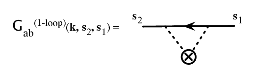
where $G_{ab}^{\rm{1loop}}(k,s_{f},s_{i})$ is the first nonlinear correction term, describing the transition into the nonlinear regime. Graphically, this term corresponds to a “one-loop” diagram (i.e. an integral over $P_{0}$), which is shown in Fig. 3.

As nonlinear effects become important $G_{ab}$ is expected to decay to zero since they erase the one-to-one correspondence of modes valid in the linear regime. This introduces a characteristic scale that describes the decay length of the two-point propagator. It was shown in [4] that this decay can be computed exactly in the high-$k$ limit, where a subset of diagrams is expected to provide the dominant contribution. Following a line of calculation that we will use again shortly, it was shown that in the large-$k$ limit,

where the characteristic decay length is determined by the rms velocity fluctuations

In [4], it is shown how to match this result valid for $k\sigma_{v}\gg 1$ to the low-$k$ behavior described by Eq. (24), to obtain a prescription for its full time and $k$ dependence. This prescription was found to be in good agreement with numerical simulations at all scales and different redshifts for density and velocity divergence propagators.

Here, we concentrate on the large-$k$ behavior of the density propagator from growing-mode initial conditions, $\Gamma^{(1)}\equiv\Gamma^{(1)}_{1b}u_{b}=G_{11}+G_{12}$ (we will henceforth use both $G$ and $\Gamma^{(1)}$ to refer to the two-point propagator). We use the algorithm presented in [4] to measure $\Gamma^{(1)}$ based on the cross-correlation property in Eq. (14). We defer a description of the simulations used here until section VI below. Figure 4 shows $\Gamma^{(1)}$ normalized by the linear growth factor $\Gamma^{(1)}_{\rm tree}=g_{11}+g_{12}$, with $g_{ab}$ the linear propagator defined in Eq. (7); the unusual notation for the growth factor is used here to emphasize that it is given by the tree-contributions to the two-point propagator, this will have a natural generalization for multi-point propagators. The figure shows $\log\Gamma^{(1)}$ vs. $\log k^{2}$ to emphasize the Gaussian decay very well predicted by Eq. (25) at all redshifts with characteristic scale given by Eq. (26).

In the following sections we investigate similar properties, regimes and measurements to those carried out with $G_{ab}$, to the case of the three-point propagator $\Gamma^{(2)}$ and, when possible, extend this to $\Gamma^{(n)}$.

To study the high-$k$ regime of the propagators, the first step is to identify the set of diagrams that is expected to dominate the large-$k$ behavior. This identification is closely linked to the concept of principal line and its generalization, the principal tree, that all the diagrams for propagators contain. These concepts are illustrated in the diagrams appearing in Fig. 5. For instance, in the top diagram there is a unique way to go from initial time (symbolized by the vertical dotted line) to the final time without crossing a $\otimes$, thus moving always in the direction of increasing time. It’s easy to check that this is true for any diagram contributing to $G_{ab}$. This is what we call its principal line.

Similarly there exists a unique tree, the principal tree, that joins the initial time to the final time in the bottom diagram of Fig. 5. The number of branches of this tree is equal to the number of points minus one for the propagator under consideration (i.e. the number of function derivatives in the definition in Eq. (17)). Again, it’s easy to check that the existence of a principal tree is general and does not depend on the number of loops that are attached to it, although at a given order different diagrams may have different principal trees (see bottom diagrams of Fig. 1). Principal trees appear then as simple generalization of the concept of principal line initially introduced in [4].

We now note that in the expansion series, all diagrams can be seen as a principal tree with loops attached to its branches. Following arguments developed in [4], we claim that the general behavior of the multi-point propagators are dominated in the large-$k$ limit by those diagrams in which every loop is directly connected to the principal tree.

This idea follows from the fact that multi-point propagators are a measure of the correlation between final and initial configurations, see Eqs. (14,22,23). And diagrams that contain only such loops are more effective in the process of correlating the final field with the initial conditions (that is, the modes running along the principal tree always interact with growing modes coming from the initial conditions). In particular, this argument remains valid at large-$k$ where these diagrams can be computed exactly, as we will show in subsequent sections.

As explicit examples, we show in the bottom diagram of Fig. 5 in dashed lines the kind of loops that contribute dominantly to the large-$k$ limit of $\Gamma^{(3)}$ (while the principal tree is represented by solid lines and the sub-dominant loops in dotted lines) . In Fig. 6 we show some of the dominant loop contributions to $\Gamma^{(2)}$, as they are the subject of next section.

These examples can be used to build a simple picture of the different loop contributions. Let us take the case of the two-point propagator. Its one-loop contribution is shown in Fig. 3. As shown in [4], this contribution is dominated by loop momenta of order $q\simeq\sigma_{v}^{-1}$, thus is in the high-$k$ limit ($k\sigma_{v}\gg 1$), most of the momentum is flowing along the principal line of the diagram. Now consider the two and higher loop contributions: the dominant loops, when resummed, give Eq. (25), again saying that all dominant loops have momenta of order $q\simeq\sigma_{v}^{-1}$ flowing in them; this is a consequence of the form of the vertices and the shape of the CDM spectrum.

As far as the subdominant loops are concerned, there are two cases at the two-loop level: with one leg in the principal line (e.g. as the dotted loop in the top half of the $G_{ab}$ diagram in Fig. 5), and with no legs in the principal line (e.g. as the dotted loop in the bottom half of the $G_{ab}$ diagram in Fig. 5). In fact, there are two types of diagrams of the latter type, depending on whether the two legs of the loop land are on the same side of $\otimes$ (as in Fig. 5), or not. The first case corresponds to renormalizing the internal propagator, the second to a renormalization of the initial power spectrum. However, since both renormalizations must be evaluated at large-scales, i.e. $q\mathrel{\mathchoice{\lower 3.6pt\vbox{\halign{$\mathsurround=0pt\displaystyle\hfill#\hfil$\cr<\crcr\sim\crcr}}}{\lower 3.6pt\vbox{\halign{$\mathsurround=0pt\textstyle\hfill#\hfil$\cr<\crcr\sim\crcr}}}{\lower 3.6pt\vbox{\halign{$\mathsurround=0pt\scriptstyle\hfill#\hfil$\cr<\crcr\sim\crcr}}}{\lower 3.6pt\vbox{\halign{$\mathsurround=0pt\scriptscriptstyle\hfill#\hfil$\cr<\crcr\sim\crcr}}}}\sigma_{v}^{-1}$, their effect on the final result must be subdominant. The subdominant loops with one leg in the principal line corresponds to renormalizing the vertex, and the level of agreement seen in Fig. 4 suggests that such vertex renormalizations are small. This corresponds to studying the three-point propagator in the limit where one incoming momentum is “soft” (of order $q\mathrel{\mathchoice{\lower 3.6pt\vbox{\halign{$\mathsurround=0pt\displaystyle\hfill#\hfil$\cr<\crcr\sim\crcr}}}{\lower 3.6pt\vbox{\halign{$\mathsurround=0pt\textstyle\hfill#\hfil$\cr<\crcr\sim\crcr}}}{\lower 3.6pt\vbox{\halign{$\mathsurround=0pt\scriptstyle\hfill#\hfil$\cr<\crcr\sim\crcr}}}{\lower 3.6pt\vbox{\halign{$\mathsurround=0pt\scriptscriptstyle\hfill#\hfil$\cr<\crcr\sim\crcr}}}}\sigma_{v}^{-1}$) while the other is large. While we are not able to resum this case, we shall see that when the whole principal tree is in the high-$k$ limit, the behavior of the three-point propagator can be established.

The aim of this section is to obtain the large-$k$ limit of the three-point propagator $\Gamma^{(2)}$ defined in Eq. (16). To this end we need to sum over the whole set of dominant loop diagrams,

that is, only consider those diagrams with loops directly attached to the principal tree, see Fig. 6. Note that to do the summation in Eq. (27) one needs to take into account the symmetry factors of each contribution ²² 2 An alternative approach has been advocated in [11] based on a Renormalization Group Theory like approach. Such a method aims at transforming discrete sums we have to deal with into a simple first order differential equation, the solution of which can be easily obtained. The two approaches are based on the same basic properties of the loop terms. We comment more on this in the appendices.. Let us start by considering the one-loop case in detail first, since it will allow an easy extrapolation when accounting for arbitrary number of loops in the large-$k$ limit.

Diagrams are computed according to the rules given in section II, but let us be a bit more precise in the notation. In Fig. 6, each of the contributing loops carries a wave vector ${\bf q}$ such that $q\simeq\sigma_{v}^{-1}\ll k_{1}$ and similarly $q\ll k_{2}$. It is connected to two segments (not necessarily distinct) taken in the set of three - denoted $(1)$, $(2)$ and $(3)$ in Fig. 6 - each carrying respectively the wave vectors ${\bf k}_{1}$, ${\bf k}_{2}$ and ${\bf k}_{3}$. In the calculation of those diagrams one has to sum over all indices, describing density and velocity divergence perturbations (we implicitly assume that such indices when repeated are summed over). As an example, we write down the corresponding integral when the loop is connected to branches $3$ and $1$,

where $s_{1},s_{2}$ are the interaction times where the loop legs attach to the principal tree, and $s^{\prime}$ is the interaction time belonging to the principal tree. Furthermore, we assumed growing mode initial conditions, so the initial spectrum $P_{ab}$ reduces to $u_{a}u_{b}P_{0}$, see Eq. (12), and $g_{ab}(s)u_{b}=e^{s}u_{a}$.

It is crucial to note that, as for the calculation of $G_{ab}$, in the high-$k$ limit the vertex matrix takes the form [4],

when contracted with an incident growing mode (such as those coming from the initial conditions). The interaction then leaves the modes along the principal tree lines unchanged and carrying the wave vector ${\bf k}_{i}$ (since ${\bf k}_{i}+{\bf q}\approx{\bf k}_{i}$) all along. As we now show, applying this large-$k$ limit to Eq. (28) simplifies calculations greatly.

Let us be general now and consider a loop that joins the segment $(i)$ and $(j)$. Again, we denote the interaction times for such a loop as $s_{1}$ and $s_{2}$. The loop contribution will eventually be given by the integration of these times over the time range of the corresponding segments. The integral over the segment ($i$) can be defined through the respective characteristic functions ${\cal I}_{i}$, with ${\cal I}_{1}(t)={\cal I}_{2}(t)=\Theta(t)\Theta(s^{\prime}-t)$ for interactions after the initial conditions but before the vertex of the principal tree (at time $s^{\prime}$) and ${\cal I}_{3}(t)=\Theta(t-s^{\prime})\Theta(s-t)$ for interactions after $s^{\prime}$ and before the time of interest $s$ ($s\geq s^{\prime}\geq 0$).

The one-loop contribution is then given by

where $s_{ij}$ is the symmetry factor associated to this contribution. It is 4 if $i\neq j$ (e.g. 2 for each incoming line), and it is only 2 for $i=j$ because the time ordering of $s_{1}$ and $s_{2}$ is ignored in Eq. (30) ³³ 3 We are able to compute time integrations ignoring time-ordering and correcting for this afterwards because the integrand (${\rm e}^{s_{1}+s_{2}}$) is symmetric under exchange of $s_{1},s_{2}$. That is, for such integrands we can take advantage of $\int_{s^{\prime}}^{s}ds_{2}\int_{s^{\prime}}^{s_{2}}ds_{1}={1\over 2}\int_{s^{\prime}}^{s}ds_{2}\int_{s^{\prime}}^{s}ds_{1}$. This symmetry arises as a consequence of the simplification of the vertex function in the high-$k$ limit, plus the linear propagator obeying $g_{ab}(s-s^{\prime})g_{bc}(s^{\prime})=g_{ac}(s)$. We will use this useful property in the summation over loops shortly, as it is more convenient to deal with an arbitrary number of integrals with the same limits.. The integral over the angles $\Omega_{q}$ is straightforward and leads to,

where $\sigma_{v}^{2}$ is defined in Eq. (26). Note that, if we could ignore the last two time integrals, the answer would be proportional to the tree-level amplitude (given by the first integral). The time integration over $s_{1}$ and $s_{2}$ can be done easily for each loop diagram characterized by $\{ij\}=\{11\},\{22\},\{33\},\{12\},\{13\},\{23\}$. When we collect all the one-loop contributions we get,

which when using that ${\bf k}_{3}={\bf k}_{1}+{\bf k}_{2}$ makes the square bracket independent of $s^{\prime}$ and leads to the remarkable result:

We are now ready to consider diagrams with an arbitrary number of loops. As we shall see it amounts to exponentiate the one-loop result above. There are at least two ways to obtain such a result. The most direct method, which we follow here, consists in computing simultaneously an arbitrary number of loops. The cumbersome part in this case is to find out the combinatorial weights for each diagram. Here we follow the one-loop strategy discussed above and ignore time ordering at first and correct for the overcounting afterwards. In Appendix A we provide an alternative derivation of this method that takes into account time ordering explicitly. A second method based on a different resummation scheme is presented in Appendix B.

The lesson we must recall from the one-loop calculation is the following. Every loop must be directly connected to two “principal” segments $(i)$ and $(j)$ of the principal tree ($i$ and $j$ go from 1 to 3, see Fig. 6). Time integration then leads to $(e^{s^{\prime}}-1)$ if $i=1$ or $2$, and $(e^{s}-e^{s^{\prime}})$ if $i=3$, and similarly for $j$. Momentum integration leads to $-\sigma_{v}^{2}\,{\bf k}_{i}\cdot{\bf k}_{j}/4$, and in addition there is an overall symmetry factor $s_{ij}$ (with $s_{ij}=4$ if $j\neq i$ and 2 otherwise).

The loop resummation in Eq. (27) relies on a proper counting of each of the diagrams that contribute in the large-$k$ limit. In turn, each of these diagrams can be defined by a set of parameters, $p_{ij}$, where each counts the number of lines connecting the segments $(i)$ and $(j)$ ($i\leq j$). For instance, the diagram in Fig. 6 corresponds to $p_{11}=1$, $p_{22}=0$, $p_{12}=1$, $p_{13}=1$, $p_{23}=0$ and $p_{33}=1$. Each loop line connects to the principal tree at time $s_{i}$. Dropping the time ordering in $s_{i}$ (within each of the principal lines), the contribution from such an ensemble of loops is given by,

In this expression the coefficient $s_{\left\{p_{ij}\right\}}$ is the symmetry factor associated with each set of $p_{ij}$. For a given ordered topology, each loop introduces a factor 4, so that

The coefficient ${{\cal M}_{\left\{p_{ij}\right\}}}$ on the other hand represents the number of times each given diagram has been computed because the time ordering has been dropped. Changing the time order (within each principal line) allows to automatically scan the different topologies (diagrams sharing the same set of $p_{ij}$) but computing them several times. The symmetry factor $p_{ij}$ in ${{\cal M}_{\left\{p_{ij}\right\}}}$ is precisely here to correct for this multiplicity factor. It is relatively easy to see that its dependence on each $p_{ij}$ factorizes, so that

where ${\cal M}(p_{ii})=2^{p_{ii}}p_{ii}!$, and ${\cal M}(p_{ij})=p_{ij}!$ if $i\neq j$ (there is an extra factor of 2 when $i=j$ to compensate for the absence of time ordering. See Fig. 7 for illustration of these symmetry factor countings). The summation over $p_{ij}$ is then straightforward and leads to exponentiations,

References

- [1] F. Bernardeau, S. Colombi, E. Gaztañaga, and R. Scoccimarro. Large-scale structure of the Universe and cosmological perturbation theory. Phys. Rep. , 367:1–3, September 2002.
- [2] A. Cooray and R. Sheth. Halo models of large scale structure. Phys. Rep. , 372:1–129, December 2002.
- [3] M. Crocce, S. Pueblas, and R. Scoccimarro. Transients from initial conditions in cosmological simulations. Mon. Not. R. Astr. Soc. , 373:369–381, November 2006.
- [4] M. Crocce and R. Scoccimarro. Memory of initial conditions in gravitational clustering. Phys. Rev. D, 73(6):063520–+, March 2006.
- [5] M. Crocce and R. Scoccimarro. Renormalized cosmological perturbation theory. Phys. Rev. D, 73(6):063519–+, March 2006.
- [6] M. Crocce and R. Scoccimarro. Nonlinear evolution of baryon acoustic oscillations. Phys. Rev. D, 77(2):023533–+, January 2008.
- [7] S. Habib, K. Heitmann, D. Higdon, C. Nakhleh, and B. Williams. Cosmic Calibration: Constraints from the Matter Power Spectrum and the Cosmic Microwave Background. ArXiv Astrophysics e-prints, February 2007.
- [8] A. J. S. Hamilton, P. Kumar, E. Lu, and A. Matthews. Reconstructing the primordial spectrum of fluctuations of the universe from the observed nonlinear clustering of galaxies. Astrophys. J. Letter, 374:L1–L4, June 1991.
- [9] Y. H. Hou, Y. P. Jing, D. H. Zhao, and G. Börner. The Nonlinear Evolution of the Bispectrum in Scale-free N-Body Simulations. Astrophys. J. , 619:667–677, 2005.
- [10] D. Huterer and M. Takada. Calibrating the nonlinear matter power spectrum: Requirements for future weak lensing surveys. Astroparticle Physics, 23:369–376, 2005.
- [11] S. Matarrese and M. Pietroni. Resumming cosmic perturbations. Journal of Cosmology and Astro-Particle Physics, 6:26–+, June 2007.
- [12] T. Matsubara. Diagrammatic Methods in Statistics and Biasing in the Large-Scale Structure of the Universe. Astrophys. J. Suppl. Ser. , 101:1–+, November 1995.
- [13] T. Matsubara. Resumming Cosmological Perturbations via the Lagrangian Picture: One-loop Results in Real Space and in Redshift Space. ArXiv e-prints, 711, November 2007.
- [14] P. McDonald. Dark matter clustering: A simple renormalization group approach. Phys. Rev. D, 75(4):043514–+, February 2007.
- [15] J. Pan, P. Coles, and I. Szapudi. Scale Transformations, Tree-level Perturbation Theory, and the Cosmological Matter Bispectrum. ArXiv e-prints, 707, July 2007.
- [16] J. A. Peacock and S. J. Dodds. Non-linear evolution of cosmological power spectra. Mon. Not. R. Astr. Soc. , 280:L19–L26, June 1996.
- [17] P. J. E. Peebles. The large-scale structure of the universe. Research supported by the National Science Foundation. Princeton, N.J., Princeton University Press, 1980. 435 p., 1980.
- [18] O. J. Rosten. A comment on the path integral approach to cosmological perturbation theory. Journal of Cosmology and Astro-Particle Physics, 1:29–+, January 2008.
- [19] R. Scoccimarro. Transients from initial conditions: a perturbative analysis. Mon. Not. R. Astr. Soc. , 299:1097–1118, October 1998.
- [20] R. Scoccimarro. A New Angle on Gravitational Clustering. In J. N. Fry, J. R. Buchler, and H. Kandrup, editors, The Onset of Nonlinearity in Cosmology, volume 927 of New York Academy Sciences Annals, pages 13–+, 2001.
- [21] R. Scoccimarro, S. Colombi, J.N. Fry, J.A. Frieman, E. Hivon, and A. Melott. Nonlinear Evolution of the Bispectrum of Cosmological Perturbations. Astrophys. J. , 496:586–604, 1998.
- [22] R. Scoccimarro and H. M. P. Couchman. A fitting formula for the non-linear evolution of the bispectrum. Mon. Not. R. Astr. Soc. , 325:1312–1316, August 2001.
- [23] R. E. Smith, J. A. Peacock, A. Jenkins, S. D. M. White, C. S. Frenk, F. R. Pearce, P. A. Thomas, G. Efstathiou, and H. M. P. Couchman. Stable clustering, the halo model and non-linear cosmological power spectra. Mon. Not. R. Astr. Soc. , 341:1311–1332, June 2003.
- [24] V. Springel. The cosmological simulation code GADGET-2. Mon. Not. R. Astr. Soc. , 364:1105–1134, December 2005.
- [25] A. Taruya and T. Hiramatsu. A Closure Theory for Nonlinear Evolution of Cosmological Power Spectra. Astrophys. J. , 674:617–635, February 2008.
- [26] P. Valageas. Large-N expansions applied to gravitational clustering. Astr. & Astrophys. , 465:725–747, April 2007.