Loss of molecules in magneto-electrostatic traps due to nonadiabatic transitions
Abstract
We analyze the dynamics of a paramagnetic, dipolar molecule in a generic “magneto-electrostatic” trap where both magnetic and electric fields may be present. The potential energy that governs the dynamics of the molecules is found using a reduced molecular model that incorporates the main features of the system. We discuss the shape of the trapping potentials for different field geometries, as well as the possibility of nonadiabatic transitions to untrapped states, i.e., the analog of Majorana transitions in a quadrupole magnetic atomic trap. Maximizing the lifetime of molecules in a trap is of great concern in current experiments, and we assess the effect of nonadiabatic transitions on obtainable trap lifetimes.
I Introduction
A primary tool for the study of ultracold matter is the magnetic trap, which can confine paramagnetic atoms on time scales of seconds. Using the techniques of laser cooling, atoms can be loaded into magnetic traps—such as the quadrupole trap created with anti-Helmholtz coils—at cold enough temperatures so that only modest magnetic field gradients are required to confine the atoms. Once loaded, the lifetime in a quadrupole trap is typically limited by collisions, thermal background radiation, or Majorana transitions [1], wherein atomic spins passing near the zero in the field minimum are not able to adiabatically follow the field direction. To such an atom, the quantization axis is lost and it may emerge from the trap zero “spin-flipped” to an untrapped state [2].
The Majorana spin-flip loss mechanism can be severe enough to quench trap lifetime before forced evaporative cooling can bring the atomic system to quantum degeneracy. Such cooling is thought to be a necessary requirement to reach the strongly correlated regimes that hold much promise for investigating novel ultracold collisions, chemistry, connections to condensed matter, and quantum information processing with particles beyond presently studied atoms, e.g., polar molecules [3]. To prevent such loss in atomic systems, evaporative cooling is instead performed in a secondary magnetic trap of the Ioffe-Pritchard or “baseball” [4, 2] configuration which does not possess a vanishing field magnitude near the trap minimum, and thereby preserves a quantization axis for all particles confined in the trap. Additional techniques to minimize Majorana loss include moving trap minima in time so that the atoms experience a non-zero field on average [5], and confining in storage rings wherein the centrifugal barrier shifts the trap center away from field minima [6]).
Large samples of molecules in their absolute rovibronic ground state have yet to be produced at temperatures below 10 mK [3]. Sample confinement therefore requires very large magnetic fields, even for the case of a quadrupole trap [7]. Electrostatic [8, 9] and magnetostatic [10, 11] traps have successfully been demonstrated for molecules, and inhomogeneous static electric and magnetic fields have been combined to increase trap depth [7]. Lifetimes have so far been limited by collisions or blackbody radiation, but once evaporative or other cooling schemes [3, 12] are employed, Majorana transitions will be a dominant cause of loss in all the currently employed traps for ground state molecules. Since the large fields necessary to create, e.g., Ioffe-Pritchard traps, are generally unobtainable, we must carefully investigate the lifetime limits imposed by Majorana transitions in the currently realizable quadrupole traps and explore possible schemes to avoid such loss mechanisms for real molecular systems.
For cold molecules that possess both magnetic and electric dipole moments, novel traps formed from both inhomogeneous magnetic and electric fields may be utilized to confine molecules in ways that mitigate the unwanted Majorana transitions. In this paper we explore the basic physics of traps for molecules in which both magnetic and electric fields are present, which we show can mitigate Majorana loss even for simple field configurations consisting of superimposed quadrupole and homogenous fields. Using a reduced, but analytically solvable, model of a molecule in both electric and magnetic fields, we explore various trap geometries that can be generated from common coil and electrode configurations. We identify the zone in the trapping potential where nonadiabatic, Majorana-like transitions can occur and we introduce approximate expressions to assess such loss. More broadly, we note that these results are of interest to the design of Stark decelerators [13], where slowed molecules experience rapidly changing field configurations. Our main focus will be on diatomic molecules governed by Hund’s coupling case (a), since in this case the electric and magnetic dipole moments are nontrivially related. In particular, we use the OH molecule as a representative molecular system, but we briefly address case (b) molecules as well.
II Molecular structure in the presence of crossed fields
Before discussing the Majorana spin-flip problem for representative traps and molecules, we first examine perturbations to the molecular structure in crossed electric and magnetic fields. We consider a diatomic, heteronuclear molecule that has a permanent electric dipole moment lying along its molecular axis. The molecule is moreover assumed to be paramagnetic, with magnetic dipole moment . In the presence of spatially varying magnetic () and electric () fields, the molecule is governed by the Hamiltonian
| (1) |
where describes the internal workings of the molecule, including lambda doubling, fine structure, and hyperfine structure, if applicable. The eigenenergies of will vary in space according the spatial variation of the fields, and these varying energies define the trap potentials.
Eigenvalues of can be constructed to any desired degree of accuracy, generating realistic trap potentials for any desired molecule. Such potentials were generated for OH in Ref. [7] according to this procedure. Presently, however, we are interested in the general features of the traps, and so will opt for a simplified molecular structure, albeit one which encapsulates all the relevant physics. We will explicitly consider Hund’s case (a) molecules with electronic symmetry (as in OH) as well as Hund’s case (b) molecules with symmetry. These electronic structures are the most commonly encountered examples of open-shell diatomics, and throughout we will neglect hyperfine structure.
II.1 Hund’s case (a) molecule
Case (a) molecules are characterized by a strong spin-orbit interaction that couples the electronic spin to the electronic orbital angular momentum, and thus also to the molecular axis. The relevant quantum numbers for a case (a) molecule are , where and are the projections of the orbital and spin angular momenta of the electrons on the molecular axis, respectively; is the total angular momentum of the molecule, resulting from the addition of the orbital and spin angular momentum of the electrons, and the rotation of the nuclei; is the projection of on the laboratory axis; and its projection on the molecular axis. We will suppress and quantum numbers which take assumed values hereafter.
In the absence of an external electric field, the molecule is also an eigenstate of parity, characterized by another quantum number, , which is conventionally denoted by and , respectively:
where is defined to be positive and the parity of the state is given by . The energy gap between these two states due to -doubling [14] is denoted by (which equals GHz for OH). OH molecules in their ground state are easily polarizable due to their relatively small -doubling and large electric dipole moment ( D). In an electric field, the superposition of opposite parity states gives rise to an effective polarization.
For simplicity, we will assume that and thus (we will suppress them also in the notation), and will consider only the four states , , and . We will further assert that the fields applied are small enough that remains approximately conserved. Unfortunately, there exists an almost complete cancelation of orbital and spin magnetic dipole moment for a molecule, leading to a nearly vanishing Zeeman interation. This deficiency in our model could be easily eliminated by considering a state, but at the expense of introducing additional levels. To maintain analytical simplicity, we will formally use a molecule, but ascribe to it a molecular g-factor of 4/5 which is the value corresponding to OH’s ground state. This ad hoc parameter adjustment will not change the qualitative conclusions of the model, as we have checked by comparison with the results for a more complicated model.
Using this molecular basis and without losing generality, we begin by assuming there is a magnetic field along the -axis at all points in space and an electric field in the -plane which makes an angle with respect to the magnetic field. The matrix elements of are easily calculated (see Appendix A):
where
| (7) |
are characteristic electric and magnetic energies and is the Bohr magneton. Geometric factors and any dependence on the particular quantum numbers of the state have been gathered into a global g-factor which can interpreted as the effective coupling with the field. Explicit expressions are given in Appendix A. This matrix can be diagonalized analytically at every point in space, yielding the following energy eigenvalues:
| (8) |
where we have assumed the existence of four different nondegenerate eigenvalues, and labeled them in increasing order of energy (i.e., “” labels the lowest energy eigenvalue). The associated eigenvectors will be denoted and . In the limit where one field vanishes, this expression reduces to the familiar Stark and Zeeman effects (see Fig. 1).


If the electric and magnetic fields are everywhere parallel, then the total energy is simply the sum of the independent Stark and Zeeman energies. In general, however, we must account for the angle between these fields. The eigenenergies are plotted versus in Figure 2 for the four states. We assume and values that correspond to our model OH molecule in fields of V/cm and G. This figure illustrates that the states experience avoided crossings in the presence of non-zero -doubling for . As we will see in further examples, such competition between electric and magnetic effects enrich the trap potentials. A semi-classical treatment of this situation is given in Appendix B.


As an aside, we note interesting features of the energies in crossed fields which may be useful in contexts beyond trapping. Applying a constant magnetic field of magnitude such that (see Fig. 1) causes two opposite parity states to be degenerate [15], as can be seen by taking the zero-electric-field limit in Eq. (8)). Because of this degeneracy, the Stark effect is immediately linear in a nonzero electric field, regardless of the angle between fields. The slope of this linear dependence, however, may depend on . This may be useful for increasing the efficiency of Stark decelerators [16].
Conversely, a Zeeman effect that is quadratic in can be obtained by applying a constant perpendicular electric field which induces an avoided crossing between two states. Rearranging terms in Eq. (8) and substituting into the eigenvalues, one can obtain . The constant electric field has induced a quadratic Zeeman effect in the vicinity of . This effect could be used to guide molecules moving in two dimensions: in a region where a linearly varying magnetic field exists, a constant perpendicular electric field, for instance, induces minima at points where the magnetic field has the value (1.5 kG for our model OH).
II.2 Hund’s case (b) molecules
Molecules like CaH, the first molecular system trapped by the buffer gas cooling method [10], or YbF, whose trapping could be useful to measure the electric dipole moment of the electron [17], belong to the category of molecules known as Hund’s case (b) [14]. We consider here a pure case (b) molecule of symmetry , in which case the electronic spin, hence the magnetic dipole moment, is completely decoupled from the molecular axis. Thus, the electric and magnetic dipoles can independently follow the external electric and magnetic fields and the net energy is the sum of the two energies. The behavior of such a molecule in a magneto-electrostatic trap does not require special attention and will not exhibit the richness of behavior enjoyed by case (a) molecules.
For real molecules, the dipoles are only approximately independent. The spin and rotational degrees of freedom are coupled by a Hamiltonian of the form , where the electronic orbital angular momentum and the rotational angular momentum of the nuclei couple to form , with projection on the internuclear axis ( in this case). couples to the electronic spin to give total angular momentum . In order to estimate its effect we can introduce the spin-rotation interaction as a perturbation. We have again built a simple analytical model including only two rotational states . In this case, the electric field is the one which lies along the axis, and we can restrict ourselves to the subset. We assume that , , and are all much smaller than the rotational spacing . With this perturbation, the energy of the ground weak field-seeking state varies as with the angle .
III Conditions for nonadiabatic transitions to untrapped states
We turn now to the nonadiabatic changes of internal state that lead to trap loss as a molecule moves through a trap minimum. Assuming an adiabatic separation in the spirit of the Born-Oppenheimer approximation, we can distinguish the “slow” center of mass coordinates of the molecule, , from the “fast” internal coordinates (denoted collectively as ). The center-of-mass coordinates can be treated classically, since typical translational energies are much bigger than the trap energy level spacing. Thus, the molecules are described by position and momentum coordinates . Adiabatic energy states are then defined parametrically at each :
where are the local energies and the corresponding eigenstates.
More generally, the internal state of the molecule is a superposition of these adiabatic states:
with . By substituting the expansion of into the time-dependent Schrödinger equation and solving for the coefficients, we find a system of coupled differential equations for the coefficients ,
| (9) |
From normalization constraints, , is the Kronecker delta function, and is Planck’s constant.
We are concerned with transitions from “trapped” states , which possess potential minima in the center of the trap, to “untrapped” states , with maxima that push the molecules far away from the trap center. The probability of undergoing a nonadiabatic transition during a process can be found to be at most the order of [18]
| (10) |
and accordingly, adiabaticity requires
| (11) |
To avoid calculating time derivatives of the states—usually a difficult task—we can recast the matrix elements using the Hellmann-Feynman theorem [19, 20],
Furthermore, the time derivative can be re-expressed in a more intuitive way using the velocity of the molecule and . The adiabaticity criterion then becomes
| (12) |
Evaluating is relatively simple once the distribution of fields is specified. Distinguishing between the different radial, polar, and azimuthal spherical components of the velocity will be useful, and we can use the expansion: , with , , and the unit vectors in radial, polar, and azimuthal directions, respectively.
As initial examples, we first examine the limiting cases of traps with either or to gain intuition before analyzing traps formed from crossed electric and magnetic fields.
III.1 Magnetostatic traps
In the case of the magnetic quadrupole trap, Eq. (12) reduces to the results well-known from previous treatments [2]. We demonstrate this assuming a magnetic field distribution , where is the magnetic field gradient on the plane. We first consider the situation in which particle’s trajectory is restricted to the -plane. Nonadiabatic transitions can connect the weak field-seeking state to the strong field-seeking state with the same parity . (The first quantum number is the parity, and denotes the projection on the local field axis throughout the remainder of this paper.) This transition probability is given by
| (13) |
and the energy gap is . As the magnetic field in this plane is given by , Eq. (11) establishes the adiabaticity criterion
| (14) |
for an azimuthal velocity at a distance from the center.
One can define a “zone of death” within which the molecule will be lost with high probability due to nonadiabatic transitions. We can roughly determine its size using the radius at which Eq. (14) becomes an equality:
| (15) |
The subscript is a reminder that these transitions occur due to the molecules’ motion in the direction, orthogonal to the local magnetic field. Spin-flips to untrapped states (Majorana transitions) are thus expected within a zone close to the center of the quadrupole distribution defined by . In this zone, the change in the orientation of the field (and thus in the adiabatic basis) is rapid when the molecule is on a trajectory close to the field zero, and the energy gap between trapped and untrapped states becomes small. Both circumstances being essential in Eq. (11), a quick change in the internal state may happen. Motion in the radial direction does not cause any transitions because the orientation of the field does not change along this direction 11 1 This does not hold true if the molecule traverses the exact field minimum. In such a case, which is of low probability, a spin-flip relative to the local direction of the magnetic field occurs due to the fast 180∘ inversion of the field direction.. Thus, the size of the zone depends on the azimuthal component of the velocity. The estimate given by Eq. (15) can also be obtained intuitively, by requiring the Larmor precession frequency (proportional to the energy gap) be less than the angular velocity (proportional to the rate of change of field orientation), which ensures that the dipole is able to adapt to the local field [5, 21].
For molecules moving in the - or -planes, the radius of the nonadiabatic zone shows the anisotropy induced by the different gradient along the axis. In general, the dependence on the polar position is given by
| (16) |
Moving across the - and -axes, this reduces to
| (17) |
and
| (18) |
The former differs from Eq. (15) due to the component of the velocity considered. The rate of change of the orientation of the field that the molecule experiences naturally depends on the direction of movement: the change is slower when moving in the azimuthal direction (on the plane, Eq. (15)) than in the polar direction, (on the plane, Eq. (18)). In summary, a different radius for the zone of death can be assigned to every direction, to every nonadiabatic transition from trapped to non-trapped state, and to every component of the velocity. For the sake of making order-of-magnitude estimates of trap loss, however, one may simply use Eq. (15) for every position and direction [5]. Finally, it is worth noting that Brink et al. [22] have recently calculated loss rates for atoms with hyperfine structure trapped in typical magnetic configurations.
III.2 Electrostatic traps
For a quadrupole electric field distribution, , with the field gradient on the plane, nonadiabatic transitions require more elaboration. There exist only two different eigenvalues and given the degeneracy we have to define a particular adiabatic basis. We will use the projection on the local field to label the vectors within each doubly-degenerate subspace, adding a subindex or to distinguish from , respectively. Specifically, the molecules are trapped in the electric weak-field-seeking states and which can make nonadiabatic transitions to the untrapped states and , which are also degenerate. The latter are lower in energy by from the trapped states at zero field (see Fig. 1).
Using the formalism presented above, we identify two types of transitions, spin conserving and spin changing, which turn out to depend on different components of velocity:
| (19) | |||||
| (20) | |||||
Note that they coincide when evaluated at the center of the trap, where the symmetry blurs the difference between radial and azimuthal velocities. Solving for the radius of the zone of nonadiabatic transitions yields for the -changing transitions:
| (21) |
This process is completely analogous to the change of in the magnetic field case, modified to accommodate the -doubling. Indeed, if , then Eq. (21) is identical to that for the magnetic case, with magnetic quantities replaced by electric ones. Motion in the azimuthal direction must be slow enough for the molecule to be able to change its dipole orientation with the local electric field. Otherwise, it will undergo a nonadiabatic transition.
Transitions which change only the parity composition but preserve depend on the radial velocity . This criterion leads to a slightly different radius for nonadiabatic transitions than that for the -changing transitions:
| (22) |
This represents a new kind of transition, foreign to the usual Majorana loss mechanism involving spins in a magnetic field. For motion in the radial direction, must be slow enough for the molecule to change its polarization adiabatically with the local electric field. In other words, the mixing of parity states and that compose the energy eigenstate must evolve because a molecule undergoing radial motion experiences a change in the magnitude of the electric field generating the quadrupole trap.
Notice that the -doubling plays a vital role in the ability of the molecule to undergo a nonadiabatic transition. Without lambda doubling, the eigenstates would be states of good for all field strengths, insuring the preservation of these states as the molecule moves radially. Moreover, nonzero -doubling smoothes the potentials near the avoided crossing, making nonadiabatic transitions less likely. Indeed, for or, equivalently, a value of larger than , nonadiabatic transitions become very unlikely. A similar expression holds for .
To highlight the difference between nonadiabatic transitions in magnetic versus electric quadrupole fields, we consider the OH radical as discussed in Ref. [7]. Using typical field strengths and molecular velocities of 10 m/s, and substituting relevant OH () energies in our model, the radius of the zone of nonadiabaticity would be 1 m for a magnetic quadrupole trap. However, such a zone does not exist at all for the electric quadrupole trap. Although not necessarily the case for all molecules, zones of death for OH in an electrostatic trap seem to be essentially negligible at the slow velocities obtainable at the terminus of a Stark decelerator. The -doubling effect eliminates this loss channel.
Loss from the electrostatic trap can also be discussed for NH in the metastable state . In this case, the -doublet is significantly smaller than in OH, leading to a larger zone of nonadiabatic transitions. We estimate that this zone is on the order of 1 m in diameter for an electric field gradient of V/cm2, which is typical for the types of experiments described in Ref. [23]. The corresponding loss rate can then be estimated as above, yielding a trap lifetime on the order of s at a temperature of 100 mK. This value is much larger than the estimated lifetime corresponding to blackbody radiation [24], and also consistent with the lifetimes found experimentally [23]. However, the lifetime decreases to 1 s when the temperature is 1 mK, and nonadiabatic loss processes will become comparable to others upon cooling to temperatures of interest.
IV Traps with crossed and fields
Upon combining and fields, both the physics of nonadiabatic transitions and its interpretation become more complicated. Because the fields are non-parallel in general, few quantum numbers are conserved, and transitions may occur from the upper trapped state to any of the three others in our model. We examine two easily-realized experimental configurations. Many more are possible, but we start here with the simplest, non-trivial examples. Namely, we will consider the influence of a uniform electric field on a magnetic quadrupole trap as well as the influence of a uniform magnetic field on an electric quadrupole trap. Nonadiabatic transition rates for these situations are found in various limits and loss rates estimated.
IV.1 Magnetic quadrupole field plus constant electric field
We first explore the consequences of crossed fields for a magnetic quadrupole trap with a constant electric field, as was the situation in the recent JILA experiment described in Ref. [7].
IV.1.1 Trap potential
In the case of an azimuthally symmetric quadrupole magnetic trap, the field distribution near the trap’s center is given by . For a simple spin-1/2 particle (i.e., ignoring lambda doubling), this results in two surfaces, one for weak-field-seeking states and one for strong-field-seeking states, which touch only in the center where . It is around this region that Majorana transitions are expected, as discussed in Section III.1. In the case of a molecule with a lambda doublet, however, there are two such sets of surfaces, offset by from one another. They can be visualized by rotating the four energy curves on the lower panel of Fig. 1 about its vertical axis. As can be also concluded from the figure, the high-field-seeking surface of parity and the low-field-seeking surface of parity become degenerate for a particular value of the magnetic field magnitude.

Introducing a constant electric field to the trap shifts the energies away from the simple, purely magnetostatic picture. Figure 3(a) shows the four adiabatic surfaces for our model OH molecule for G/cm and V/cm, with eigenenergies given by Eq. (8). They are denoted by , , , and , using the name of the corresponding eigenvectors. These surfaces are depicted as slices through the center of the trap where . The upper two surfaces and the lower two remain degenerate at , with energies given by the Stark eigenvalues
| (23) |
where (a subindex is added to emphasize that the electric field is constant in space). The electric field breaks the cylindrical symmetry of the pure magnetic quadrupole trap. Thus, the highest energy surface, , possesses roughly elliptical contours of energy (Figure 3(b)). Note that the trap is not harmonic, but linear in the center.
The second-highest energy surface, , which is also able to trap molecules, has a double-well structure due to two conical crossings with the next surface, , and which occur at the coordinates . At these particular points, electric and magnetic fields are collinear and the surfaces can cross. The crossing is avoided for any other angular configuration, which leads to the conical structure. Thus, while an interesting trap geometry may be generated, nonadiabatic transitions may be possible at these type of points. However, we only discuss loss in the central region of the magnetic quadrupole trap.
IV.1.2 Losses

As a result of adding the constant electric field to the magnetic quadrupole field, nonadiabatic transitions may occur between and as in the purely magnetic case, but now transitions from and are possible due to the electric field.
We begin with . Using , the condition for adiabaticity when moving on the -plane (with the electric field along the -axis) is:
| (24) |
This criterion is always satisfied in the limit , which reduces to the pure magnetic quadrupole field case where there is no such transition. To gain insight from this expression, we can assume that the effects from the magnetic field are small near the center of the trap (). This results in the simple expression
| (25) |
The combination can be easily identified as the component () of the velocity that is perpendicular to the electric field, which is along . Thus, Eq. (25) can be re-expressed as
| (26) |
which may be numerically evaluated in a particular trap to check if this transition leads to losses. In fact, the maximum of the left-hand side of the previous expression as a function of is given by , which turns out to be neglectable for realistic traps containing OH.
Analytical expressions analogous to Eq. (24) can be obtained for the other two transitions, but their exact form is complicated and we do not present them here. Instead, since these transitions are expected to occur near the center of the trap, we can assume that the magnetic field interaction there is weaker than the electric field interaction. We thus consider the magnetic field as a perturbation. The degeneracy of the eigenvalues makes it convenient to use Brillouin-Wigner perturbation theory [25, 26] and a zero-order basis which diagonalizes the Zeeman perturbation on each parity subset separately. For example, Eq. (25) coincides with the expression obtained using perturbation theory when keeping only leading terms for each member of Eq. (12). For the perturbative series to converge, the condition has to be fulfilled.
Using the perturbation approach to estimate the transition rate for , which is azimuthal, we find it is less likely to occur than the transitions because the transition probability is of higher order while the energy gap remains nearly the same. Therefore, condition 26 should set a bound on these losses as well.
The remaining transition, , is the only one possible in the absence of an electric field (see Eq. (15)). Perturbation theory shows that the previously circular zone of nonadiablatic transitions now becomes elliptical. The latter is given in polar coordinates by
| (27) |
Note that this reduces to Eq. (15) in the absence of an electric field. Substitution of in the previous expression allows for the calculation of the semi-axes of the ellipse (i.e., along the - and -axes). The circular zone of nonadiabatic transitions shrinks along the external electric field and extends in the perpendicular direction.
Assuming that the -axis (also being perpendicular to the -axis) radius of death is analogous to (except for a scaling factor due to the doubled gradient), we can estimate the scaling of the total losses as a function of the electric field magnitude. From the previous expressions, we see that losses occur within a completely asymmetric ellipsoidal zone. The flux of molecules through this ellipsoid per time unit constitutes an estimate of the loss rate. For low values of the electric field magnitude , the eccentricity of the ellipse in the plane is given by . If we approximate the ellipsoid and the molecular cloud with spheres [5], then losses due to the transition would be of the same order of magnitude as in the pure magnetic quadrupole trap, with corrections on the order of .
In conclusion, for electric field magnitudes satisfying both and Eq. (26), the addition of a constant electric field to the trap does not increase the rate of losses due to nonadiabatic transitions beyond that expected from a magnetic quadrupole trap.
IV.2 Electric quadrupole field plus constant magnetic field
The final crossed-field configuration we will examine is that of a electric quadrupole field combined with a constant magnetic field. We examine the losses in this situation in the same manner described above.
IV.2.1 Trap potential
We again consider an electric quadrupole field configuration with field distribution , where the gradient is constant. In the absence of a magnetic field, there are only two (doubly degenerate) distinct surfaces, one weak-field-seeking and one strong-field-seeking, and the -doublet prevents a connection between the surfaces in the center of the trap. They can be visualized by rotating the two energy curves in Fig. 1(b). The primary effect of adding a small constant magnetic field, , is to break the degeneracy. Higher magnetic fields can modify the connections between different potential energy surfaces. For example, tuning the magnetic field can bring regions of surfaces closer to degeneracy, which can induce linear Stark dependence along the directions perpendicular to , as discussed in Section II.1, or induce conical intersections similar to those in Fig. 3.
The surfaces in Fig. 4 correspond to our model OH molecule and are generated for fields of V/cm2, G. This magnetic field is small enough that no crossings occur between the middle two surfaces, and the two trapping surfaces are harmonic. The upper surface is characterized by the following spring constants: , , and , where (the subindex “0” is added to indicate a constant magnetic field).
IV.2.2 Losses
Exact expressions can be found for the probabilities of nonadiabatic transitions out of the trapping state, . The adiabaticity criterion for transitions is:
| (28) |
For a general , which is the angle that the electric field makes with the constant magnetic field (assumed to lie along the -axis), this relation converges to the analogous expressions for the pure electric trap (see Eq. ( 19) and (20)) when goes to zero (we do not present the details of the necessary transformations here, complicated by a location-dependent change of basis).
In the case of the azimuthal term in Eq. (28) being alone, the ratio of the energy gap to the transition probability, thus the adiabaticity, would increase at every point with the addition of a magnetic field, but the contribution of the radial term seems to depend on the distance. The analysis for points very close to the center of the trap () shows that the ratio between the left- and right-hand sides of Eq. (28) scales as . As a result, the nonadiabatic transition is actually hindered by increasing the magnetic field.
Expressions analogous to Eq. (28) can be obtained for the other two transitions ( and ), but the lengthy analysis will not be presented here. We therefore apply Brillouin-Wigner perturbation theory again to consider the electric quadrupole field as a perturbation to the homogeneous magnetic field near the trap center. This perturbation theory shows that the transition depends on both the radial and azimuthal velocities. Close to the trap center, both the transition probability and the gap between the potential energy surfaces do not change noticeably due to the addition of the constant magnetic field. Dependence with the latter appears only in second-order terms in the perturbation, , far from the center. Thus losses due to this transition are not expected to be very different than the ones in the pure electric quadrupole trap. However, numerical estimates using the exact expressions show that the presence of the magnetic field may inhibit the corresponding spin-flips.
Finally, we consider the transition . The magnetic field breaks the degeneracy in the upper subspace and nonzero transition probabilities due to both radial and azimuthal motion connect both states. Given the confining character of state they do not lead to trap losses. Regardless, while the transition probabilities (which connected already the degenerate states in the pure electric quadrupole for the analogous choice of basis) remains essentially constant, the gap increases linearly with the addition of the magnetic field. Thus these flips are again hindered by the presence of the additional field.
In conclusion, the addition of a constant magnetic field to an electric quadrupole decreases trap losses beyond those found in a pure electric quadrupole trap. In the previous analysis we have assumed tiered surfaces like that shown in Fig. 4, where (magnetic field less than 1.5 kG for our model OH molecule). Degeneracies and crossings between surfaces and that occur at higher magnetic fields might deserve special attention.
V Remarks on Stark deceleration of OH
The Stark deceleration technique, an experimental scheme to obtain samples of cold polar molecules [13], relies also on the absence of significant nonadiabatic transitions when switching from one electric field stage to the next. Molecules transferred to the wrong states would not experience the proper transverse focusing and slowing and the molecular packet would disintegrate. We can apply the formalism above with only minor modifications to analyze the Stark deceleration process, and in particular, its application to OH in the state [27].
As the molecule moves along the decelerator, it experiences brisk changes in the local field. As a result, the field orientation and strength may change, giving rise to non-vanishing derivatives and . Eqs. (19) and (20) can be modified to include them in our model:
| (29) | |||||
| (30) | |||||
The changes in the local field are maximum when the voltage is switched between pairs of electrodes. We estimate these based on the Stark decelerator and electrostatic trap of the Lewandowski group at JILA [28]. During a switching time of 1 s, the modulus of the local field at the midpoint of a pair of electrodes decreases a factor of 30 while rotating by . Assuming that the molecule is essentially motionless during this process, this yields maximum values of rad/s and Vcm-1s-1. Introducing in Eq. (10) the derivatives given by Eq. (29) and (30), we find nonadiabatic probabilities of the order of for OH. For NH in the metastable state, another Stark decelerated molecule of interest [23, 28], the contribution due to the change of modulus (calculated using Eq. (30)) is several orders of magnitude smaller. Thus, nonadiabatic transitions are negligible in the decelerator, a conclusion in agreement with the findings of [23].
VI Conclusions
The presence of both permanent magnetic and electric dipoles in case (a) molecules opens the way to rich trap dynamics, intrinsically different than that more commonly found in atomic systems. The experimental exploration of their behaviour and the potential control of their dynamics, which could be exploited through the use of arbitrary superpositions of electric and magnetic fields, is a question of great importance to current experimental research. In particular, we have shown how the simultaneous presence of both fields can lead to new spatial distributions within the trap. Also, while homogeneous electric fields open new nonadiabatic connections between states in a magnetic quadrupole trap, constant magnetic fields can inhibit losses in an electric quadrupole trap. In summary, for practical design of magneto-electrostatic traps, such as those experimentally explored in Ref. [7], it should be noted that crossed electric and magnetic fields effect can be used to inhibit previously existing nonadiabatic transitions by increasing the energy gaps between surfaces or to enhance those transitions by introducing new depolarization pathways. The suitable design of the field parameters in magneto-electrostatic traps can reduce nonadiabatic transition loss rates below other limiting loss mechanisms, and thereby open new avenues for explorations of ultracold molecular physics without the need for building unwieldy Ioffe-Pritchard traps.
The comparative analysis of nonadiabatic transitions in pure magnetic and electric distributions has also allowed the identification of a new type of nonadiabatic transition in changing electric fields, foreign to the usual Majorana loss mechanism. Namely, nonadiabatic transition due to the change of magnitude of the electric field and not due to its orientation, and this effect is intrinsically linked to the presence of the avoided crossing induced by the -doubling.
We also remark that Hund’s case (b) molecules are unaffected by the new nonadiabatic loss mechanisms that appear in Hund’s case (a) molecules, and therefore may be more attractive for certain applications.
Acknowledgements.
ML and JLB gratefully acknowledge support from the NSF and the W. M. Keck Foundation, and BLL from the NRC. We thank J. Ye, H. Lewandowski, B. Sawyer, E. Hudson, E. Meyer and S. Y. T. van de Meerakker for helpful discussions.Appendix A Stark and Zeeman interactions in crossed fields
When external - and -fields do not form a shared quantization axis, the scalar products which define Zeeman and Stark interaction terms have to be evaluated for general electric and magnetic vectors. We outline how matrix elements of the Hamiltonian in Eq. (1) may be calculated in these cases. Both electric and magnetic dipole moments are naturally expressed in the molecular frame, whose -axis coincides with the molecular axis. The electric dipole moment lies along the molecular axis while the magnetic one is easily calculated using electronic operators that are referenced to the molecular frame. Fields, on the other hand, are best expressed in the laboratory frame. The evaluation of the scalar products which define Stark and Zeeman interaction thus requires the expression of dipoles and fields in the same reference system, which we can choose as the laboratory reference system. Changing the spherical components of the dipole moments from the molecular to the laboratory frame involves the use of Wigner matrix elements ().
Using these notions, the Zeeman and Stark interaction terms can be expressed as:
| (31) |
where and represent the dipole and the field, respectively. As the electric dipole moment lies along the internuclear axis, its spherical coordinates in the molecular frame can be expressed as . If the contributions of the out-of-axis components of the magnetic dipole moment are negligible, as we have assumed in the text, is also obtained. Thus, the interaction term 31 reduces to
| (32) |
Matrix elements for the interaction operators can be evaluated using the following expression, in the basis without parity:
which, after some algebra, allows one to obtain the following elements in the parity defined basis:
and
| (43) |
where the relation allows one to choose the correct signs of and components in the previous expression. The difference in the parity factor in both expressions is related to the magnetic dipole moment not being a constant (as is ), but an operator. The evaluation of the latter——in the parity basis extracts different signs when acting on the different signed components.
Appendix B Semiclassical analog for Hund’s case (a) molecules
The competition between the electric and magnetic effects that determines the potential energy surfaces can be illustrated by a simple analogy that provides useful intuition. The electric dipole moment lies parallel to the molecular axis. For a case (a) molecule, the magnetic dipole is also constrained to lie along this axis, on average, due to strong spin-orbit coupling. Each field will thus try to orient the molecule along itself.
It is reasonable to imagine that the system will essentially align to the stronger field. That being the case, when rotating the smaller field by varying and holding the magnitudes of both fields fixed, the molecular axis will remain anchored to the stronger field while the interaction with the smaller field would vary as the projection of the dipole on the smaller field, . In fact, dependences of the form and can be extracted from Eq. (8) in the limit of very small .
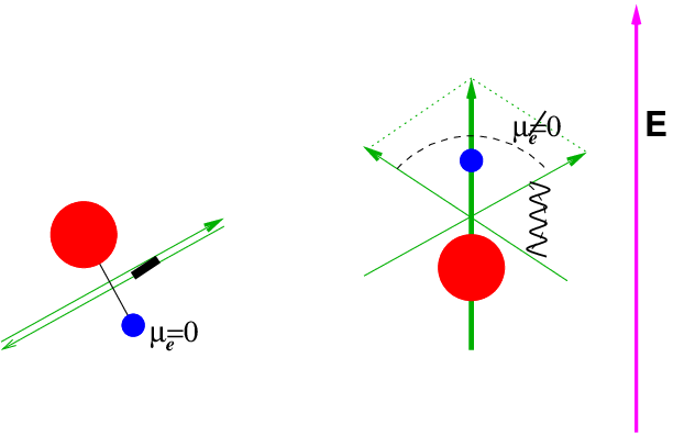
A semiclassical model can also be found for the case in which both fields exert a similar force on the molecule. As illustrated in the righthand drawing of Figure 2, if the molecular axis makes an angle with respect to , then it makes an angle with respect to , and the resulting energy as a function of orientation is
Minimizing (maximizing) this energy with respect to provides the energies given in Eq. (8) in the absence of -doubling. The acounts for the relative orientation of the electric and magnetic dipoles.
To include the effect of -doubling, we imagine that the molecule consists of two, instead of one, antiparallel electric dipoles in zero electric field. This corresponds to the fact that the molecule in zero field experiences no net dipole moment. As the field is turned on, both electric dipoles tend to align with the field, but are counterbalanced by a fictitious spring that acts to keep them antiparallel (see Fig. 5). The spring serves to reproduce the -doublet in this model. If the angle between the two electric dipoles is denoted , then this “scissors” model can be described by a classical energy
| (49) |
where we have introduced particular dependences on of both the molecule electric dipole moment and the energy of the imaginary spring. The extrema of this function constitute a good approximation to the quantum energies except that they cannot reproduce the avoided crossing.
References
- [1] E. Majorana, Il Nuovo Cimento 9, 43 (1932).
- [2] H. J. Metcalf and P. van der Straten, Laser Cooling and Trapping (Springer-Verlag, New York, 1999).
- [3] J. Doyle, B. Friedrich, R. Krems, and F. Masnou-Seeuws, Eur. Phys. J. D 31, 149 (2004).
- [4] T. H. Bergeman, P. McNicholl, J. Kyacia, H. Metcalf, and N. L. Balaz, J. Opt. Soc. Am. B 6, 2249 (1989).
- [5] W. Petrich, M. H. Anderson, J. R. Ensher, and E. A. Cornell, Phys. Rev. Lett. 74, 3352 (1995).
- [6] F. M. H. Crompvoets, H. L. Bethlem, R. T. Jongmaand, and G. Meijer, Nature 411, 174 (2001).
- [7] B. C. Sawyer, B. L. Lev, E. R. Hudson, B. K. Stuhl, M. Lara, J. Bohn, and J. Ye, Phys. Rev. Lett. 98, 253002 (2007a).
- [8] S. van de Meerakker, P. H. Smeets, N. Vanhaecke, R. T. Jongma, and G. Meijer, Phys. Rev. Lett. 94, 023004 (2005).
- [9] T. Rieger, T. Junglen, S. A. Rangwala, P. W. H. Pinkse, and G. Rempe, Phys. Rev. Lett. 95, 173002 (2005).
- [10] J. Weinstein, R. deCarvalho, T. Guillet, B. Friedrich, and J. M. Doyle, Nature (London) 395, 148 (1998).
- [11] W. C. Campbell, E. Tsikata, H. Lu, and J. M. Doyle, Phys. Rev. Lett. 98, 213001 (2007).
- [12] B. L. Lev, A. Vukics, E. Hudson, B. Sawyer, P. Domokos, H. Ritsch, and J. Ye, Phys. Rev. A 77, 023402 (2008).
- [13] H.L. Bethlem, G. Berden, and G. Meijer, Phys. Rev. Lett. 83, 1558 (1999).
- [14] J. Brown and A. Carrington, Rotational Spectroscopy of Diatomic Molecules (Cambridge University Press, 2003).
- [15] A. Boca and B. Friedrich, J. Chem. Phys. 112, 3609 (2000).
- [16] B. C. Sawyer, B. K. Stuhl, B. L. Lev, J. Ye, and E. R. Hudson (2007b), arXiv:0705.3442.
- [17] J. J. Hudson, B. E. Sauer, M. R. Tarbutt, and E. A. Hinds, Phys. Rev. Lett. 89, 023003 (2002).
- [18] A. Messiah, Mechaniqué Quantique (Dunod, Paris, 1984).
- [19] H. Hellmann, Einfuhrung in die Quantenchemie (Deuieke, Leipzig, 1937).
- [20] R. P. Feynman, Phys Rev. 56, 340 (1939).
- [21] W. Ketterle and N. J. van Druten, Adv. At. Mol. Opt. Phys. 37, 181 (1996).
- [22] D. M. Brink and C. V. Sukumar, Phys. Rev. A 74, 035401 (2006a).
- [23] S. Hoekstra, M. Metsala, P. C. Zieger, L. Scharfenberg, J. J. Gilijamse, G. Meijer, and S. Y. T. van de Meerakker, Phys. Rev. A 76, 063408 (2007a).
- [24] S. Hoekstra, J. J. Gilijamse, B. Sartakov, N. Vanhaecke, L. Scharfenberg, S. Y. T. van de Meerakker, and G. Meijer, Phys. Rev. Lett. 98, 133001 (2007b).
- [25] L. Brillouin, J. Phys. Radium. 3, 373 (1932).
- [26] E. P. Wigner, Math. Naturw. Anz. ungar. Akad. Wiss. 53, 475 (1935).
- [27] J. Bochinski, E. R. Hudson, H. J. Lewandowski, and J. Ye, Phys. Rev. Lett. 91, 243001 (2003).
- [28] H. Lewandowski, Private communication. (2007).