Quantavo: a Maple Toolbox for Linear Quantum Optics
Abstract
This manual describes the basic objectives, functionalities and uses of the toolbox for Maple (MaplesoftTM) called Quantavo. It is intended to facilitate calculations both symbolically and numerically related to Quantum Optics. In particular the evolution, measurement and entanglement properties of quantum states in the Fock basis can be simulated with it. It is provided to the community as a free open source module.
1 Objectives
The toolbox is made to be used with the following approach:
Declare an initial state, let it evolve through a quantum optical circuit involving
linear optics (LO) and measurements and finally ask various questions about the structure, entanglement,
and properties of the final state.
The toolbox intends to do so providing:
A) A framework in which to declare, manipulate and characterize quantum states
of light (finite number of modes, and finite dimensional).
B) Procedures that implement linear operations or whole linear optics circuits on our states such as:
- •
Beam Splitters (BS)
- •
Phase Shifters (PS).
- •
arbitrary unitary transformations of the modes.
C) Procedures that implement arbitrary measurements (both projective
or generalized positive operator valued measures (POVM)).
D) Procedures to determine probabilities and expected values for projective measurements
and POVM measurements.
E) Procedures to trace out measured or inaccessible modes.
F) Procedures to calculate different entanglement measures such as:
- •
Entropy of entanglement
- •
partial trace, norm Negativity, Logarithmic Negativity
G) Access to properties such as the mean Energy of given states.
H) Extract and display lists of coefficients along with their indexes like:
H) Tools to easily plot states and density matrices.
2 Getting Started
Some previous knowledge about Maple from MaplesoftTM is required to use this tool. However, the brief “Take a Tour of Maple” should suffice to get started. This toolbox works with Maple 9.5, Maple 10 and Maple 11.
2.1 Definitions and Notation
Procedures: Formally, in Maple, a procedure definition is a valid expression that can be assigned to a name. The procedures we will use can be thought of as a set of “rules” that generally receive one or more inputs and return one or more outputs. We will write them in typewriter face. For example the procedure IsHermitian(M) evaluates if a Matrix M describing a density matrix is hermitian. A dictionary with all the procedures involved in Quantavo can be found in the appendix.
Modules: Modules are repositories of procedures. By loading a module we can use its procedures in the
Maple worksheet. For example Quantavo is the module containing the procedures we will use.
objects: The objects in which we will encode our quantum states will be written in bold
face. These will include vec, mat, matcol and poly and will be introduced later.
d and K: Throughout the manual, ‘’ will stand for the number of modes and ‘’ for the
dimension of each mode. If considering the photon number degree of freedom, then ‘’ will be the maximum number of photons in any mode. It is important to keep track of the value of these two
global variables throughout the worksheet as they play an important role in the labelling of the optical modes and translation procedures. These variables can always be updated and displayed with the procedure: findKnd(State).
2.2 Loading the Modules
All necessary files can be found at,
http://www.imperial.ac.uk/quantuminformation/research/downloads
- 1.
uncompress the file Quantavo.zip.
- 2.
Save the folder QUANTAVO to a given directory. It should contain the files Quantavo.mpl and Quantavo_Example_Worksheet.mw.
- 3.
One can start opening the worksheet Quantavo_Example_Worksheet.mw.
- 4.
To use the module in a new worksheet execute the following commands 11 1 note that if the new file is in a different directory it should be,
read “/path-to-folder/QUANTAVO/Quantavo.mpl”;
or under MS Windows,
read “C:path-to-folderQUANTAVOQuantavo.mpl”; :
- 5.
You are ready to use Quantavo !
Note that You may also save the module to your Maple library. To do so, visit the maple help on module, savelibname and savelib.
3 Toolbox
To run Quantavo one has to load the following modules:
- •
LinearAlgebra (Linear Algebra package from MaplesoftTM built in Maple)
- •
Quantavo (General toolbox)
Additionally, if we want to plot our states we will also need the module
- •
geom3d (geometry package from MaplesoftTM built in Maple)
- •
plots (plotting package from MaplesoftTM built in Maple)
3.1 Objects and Operations
When quantum optical states have a few modes and live in high dimensions, the matrices or vectors describing them very soon become intractable. To mitigate this difficulty, the procedures from Quantavo store and manipulate only the non-zero elements in the description of our states. Our main objects will be 2 column and 3 column matrices.
3.1.1 Pure States
Two column objects will describe vectors in Hilbert space of the form:
Where all indices “” range from . Pure state vectors will be encoded in 2 column matrices that we will call trimmed vectors containing only non-zero entries. They will only contain non-zero entries. These objects will be named as a short vector: “vec” and will have the following appearance:
For each row, the second column will be a list with the number of photons in each mode, This way [0,1,2] stands for . the first column will contain the coefficient associated with this ket. The whole will describe the linear supperposition of all these kets with their coefficients, therefore the above describes the unnormalized quantum state:
3.1.2 Mixed States
Two objects will be used to display density matrices. The first one is a square matrix, with as little zero entries as possible. This matrix will be called “mat” and will have for the above state the following form:
Another object that can also describe a density matrix will be a 3 column matrix, or trimmed density matrix. It will be named as a short column matrix: “matcol”. The second column will be a list with the number of photons in each mode of the ket. This way, [0,1] in the 2nd column describes . The third column will be a list with the number of photons in each mode of the bra; therefore [2,1] in the 3rd column describes . Finally The first column will have the coefficient associated with this ketbra . The whole will describe the non zero elements of the density matrix. As an example consider the above state which will be:
Summarising, we will use mainly 3 objects: vec, mat and matcol.
A fourth object less commonly used is a polynomial representation of the state. It is a polynomial in the mode operators that define the state. A general state would then be:
and its description as a poly object:
(note that the commutation relations are not taken care of in poly objects).
3.2 Declare, Propagate, Measure and Ask
Quantavo contains various procedures that allow problems to be formulated as follows:
- 1.
Declare the initial state.
- 2.
Apply different transformations to it (Beam Splitter, Phase Shifter, Arbitrary Unitary, …).
- 3.
Measure certain modes (and trace out the inaccessible ones), find out probabilities.
- 4.
Ask different questions about the properties of the state: Display, Plot, evaluate certain measures of Entanglement, etc..
Additionally, the order in which we use these procedures can be changed and the questions in item (4) can be formulated at any intermediate time. In addition, more states can be tensored or added at later times. Finally there are procedures to interconvert mat, vec, matcol and poly. Let us then give a more detailed description of these four basic steps.
3.2.1 Declaration
There are different ways to declare a state, all depending on its characteristics.
Pure States
For pure states of known functional form. That is, if we have a state of the form:
| (1) |
and we know explicitly we may use the following structure:
Declare the number of modes “”, the maximum number of photons “”, and make a loop to declare the elements. For example:
In this case it is easy to declare the object vec directly as:
we can use:
Mixed States
The generalized states (either pure or mixed) we are interested in can be written as:
| (2) |
where and stand for and respectively.
The density matrix for these states is dimensional which is in general
too large for the computer to handle. We will therefore describe these states using mat, matcol or poly.
objects.
Two main strategies can be used to declare our states:
- 1.
If our starting state is pure and will become mixed later, we can declare a pure vec object and then convert it into a mat or matcol when needed. All procedures to convert are named in the intuitive way: “object2object”. This way to convert vec into mat we have the procedure vec2mat, to convert mat into matcol, mat2matcol and so on for all objects and conversions. Therefore, once our pure state vector V has been declared we can do the following:
- 2.
if our starting state is mixed to begin with, we can declare our initial state as the object mat or matcol. To do so, if we know the functional form of in eq.(2) then we may directly declare our state. For example to declare the state:
We could use:
or
or yet again, meaning
The basic conclusion is that there is no single way of declaring our state
and that depending on its structure we have to find a clever way of declaring it.
As a general guideline, small states without an obvious functional structure can be declared
giving all elements. Medium sized pure states can be declared using a clever loop, ‘trimmed’
and transformed to vec, mat or matcol.
It is worth noting that when using the built-in declaration procedures such as
SqueezedVac, CoherentState, TensorVac, Vac,
or the inter-converting ones like mat2matcol, mat2poly, vec2mat, etc, the values of and are automatically updated. However, if the states are declared
from scratch, the values of and should be explicitly declared. Applying to our
state the procedure findKnd() can help troubleshoot by reevaluating the value of these global variables.
3.2.2 Evolution
Beam Splitter
We can apply a beam splitter to a vec or matcol state V with the BS procedure:
Where i, j specify which modes the beam splitter acts on. It is therefore essential to carefully label the modes of our quantum optical circuit. This will effectively do the following mode transformation:
| (3) |
Leaving ‘’ and ‘’ as unevaluated variables. If we want to use different reflectivities and transmittivities for our Beam Splitter (variables or numbers) we may use myBS and input ‘’ and ‘’ as follows:
Further details about its use can be found in the example in section (4)
Phase Shifter
The phase shifter procedure (PS) can be used with mixed and pure states:
| (18) | |||
| (19) |
Build Unitary
If we wish to construct a unitary matrix that transforms the modes of light and describes a given linear optics (LO) circuit we may use the procedure BuildUnitary. Together with UnitaryEvolution it will evolve the state through a given LO circuit. To build a unitary consisting of Beam Splitters (BS) and Phase Shifters (PS) we will do the following:
In general, in our list of lists, lists with 4 elements, like [i, j, t, r] build BS transformations between
modes i and j, lists with 3 elements like [i, j, t] build BS transformations for modes and such that , and lists
with two elements like [i, ] build PS transformations on mode i.
UnitaryEvolution
Whether we have just built a unitary matrix with BuildUnitary or we have a arbitrary unitary matrix to
transform our modes , we can use this procedure as follows:
3.2.3 Measurement
The Project Procedure:
If we wish to know the state after a projective measurement we may use the procedure
Project. Depending on the inputs we give to the procedure it will
do a projective measurement and return a density matrix (matcol) or state vector (vec). Below is a
description of its different uses:
- 1.
if given (vec1, list, vec2) and say vec1 and vec2 describe respectively and , Project(vec1, list, vec2) returns the vec (in principle unnormalized) corresponding to the expresion:
As an example consider list=[2,3] meaning that we want to measure modes two an three. The vec object that corresponds to the projector must therefore have kets with 2 modes.
For example, if isand is
Then,
- 2.
if given (matcol 1, list, vec 2) and say matcol 1 and vec 2 describe and then it will return the matcol object:
So for example, taking the same V2 as above and the Kraus Operator (or projector):
Then,
which is the density matrix corresponding to:
- 3.
if given (vec 1, list, matcol 2) and say vec 1, matcol 2 describe and respectively, then it will build and return the matcol object corresponding to:
- 4.
if given (matcol 1, list, matcol 2) and say matcol 1 and matcol 2 describe and respectively, then it will return:
(see further down for POVM measurements)
In a nutshell:
Project(, list, )
Project(, list, )
Project(, list,)
Project(, list,)
If we encounter a destructive measurement, it is possible to trace out the measured modes
with the Traceout procedure (cf. appendix). Also POVMresult traces out
the measured modes (see next section). We may otherwise calculate the full
trace of a mat or matcol object with StateTrace or multiply vec and matcol
in different orders thanks to StateMultiply.
The Probability Procedure:
This procedure will calculate the probability of a measurement result or an expected value.
It considers the same cases and objects as the above Project procedure.
It uses the definition,
and assumes that safisfy and to calculate probabilities.
Therefore, one should verify that these conditions hold for the matrices
describing in order to obtain meaningful probabilities.
Below we show more details for different inputs:
Probability(, list, )
where (, ) are converted to matcol objects in an intermediate
step. One should pay attention to the choice of the projection operator . If it is
not nomalized it can give unphysical values for the probability.
Now for a given POVM or Projector,
Probability(, list, )
Or given a vec and a density operator matcol:
Probability(, list, )
where has been converted to a matcol object.
And finally for a POVM and a density operator:
Probability(, list, )
3.2.4 POVM measurements
Quantavo posesses a procedure to describe POVM measurements. If our state before the measurement is or , and the POVM elements are described by the set , satifying and . Then the state after the measurement will be:
or
assuming or .
This will be implemented by the procedure POVMresult
which will take as inputs,
POVMresult(matcol, , matcol/vec)
and implement the operation,
POVMresult(, , )
=
where ‘’ are all the indexes not included in ‘’.
3.2.5 Declaring POVMs
The matcol objects that represent POVM operators need to be declared.
One option is to declare them as standard states and convert them to matcol.
Since avalanche photo diode detectors (APDs) are a standard tool in quantum optics,
an interactive tool to declare them is also provided. Executing,
and choosing (1, r, 4) will return,
recovering the expected . Note the convention
for the BS in front of the detector for which is a perfect detector and .
These are therefore the main tools to describe and simulate quantum measurements in this framework.
3.2.6 State Properties
Some questions that will interest us will concern hermiticity, normalization and
entanglement measures. So far, Quantavo has the following usefull procedures:
IsHermitian to check for selfadjointness,
IsNormalized to check for normalization,
StateNormalize to normalize mat, matcol or vec
StatePartialTranspose to partial transpose
Negativity to calculate the negativity as the sum of all negative eigenvalues
of the partial transposed density matrix.
LogNegativity to calculate the Logarithmic Negativity.
StateApprox to do symbolic or numeric approximations transforming our matcol or vec state.
For practical examples on how to use them one can refer to the following section. Otherwise, a detailed dictionary of procedures can be found in the appendix.
4 Practical Example
4.1 Squeezed state photon subtraction

Our initial state is a pure two mode squeezed state that
can be described by
.
We would like to declare it and propagate it through the circuit presented in fig. 1.
We observe that our initial state has three modes, one of which is a vacuum mode.
We can work out as an example the state with up to 4 photons:
We then apply the corresponding Beamsplitter transformation (if “” changes from
the BS transformation, it is automatically recalculated after the BS operation and reset
to its new value. In this case it doesn’t change).
Measurements:
First we will consider the case of a perfect photon number resolving detector.
The projector can simply be introduced as:
We may now trace-out the measured mode. Tracing out can
then be done as follows:
We may also simulate a measurement with an avalanche photo-diode described by the Kraus Operator: . That is, if the state “V1” represents the state , we want to find the state resulting from the measurement:
For this simple example we have at most 4 photons so we will approximate .
Therefore to measure mode we construct the associated POVM which can then be expressed as a matcol object:
See the dictionary in the appendix for details on how to use the StateApprox procedure.
Entanglement
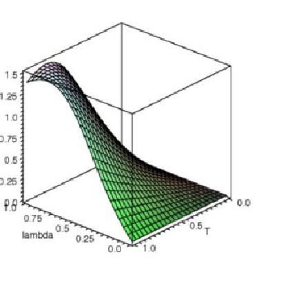
We may now compute different properties of this state as for example the Negativity. We take
the state after the detection of exactly one photon and obtain:
The eigenvalues can be hard to find if our state has symbolic
entries with complex conjugation. A previous simplification (assuming
real variables) can help, but other solutions are possible.
This explicit expression allows us to plot different values of the negativity for
various ranges of parameters:
Further details, examples and documentation can be found on the website of the
Imperial College London quantum information group,
http://www.imperial.ac.uk/quantuminformation/research/downloads
Acknowledgements
This project was supported by EPSRC grant EP/C546237/1 and by the Integrated Project Qubit Applications (QAP) supported by the IST directorate as Contract Number 015848. The author would also like to thank Alain Le Stang and the members of Mapleprimes.com for useful suggestions.
Appendix A Dictionary of procedures:
A quick reference list is provided and an alphabetically ordered
dictionary follows.
Objects
Appearance
Declaration
vec
vec:=CoherentState(K,d,)
vec:=SqueezedVac(K,d,)
vac:=Vac(K);
vec1:=TensorVac(vec,m)
vec1:=TensorProduct(V,[1,2],W,[3,4])
vec:=Trim(V)
mat
mat:=vec2mat(vec)
mat:=matcol2mat(matcol)
or direct declaration of the
Matrix
matcol
matcol:=vec2matcol(vec)
matcol:=mat2matcol(mat)
or direct declaration of the
3 column Matrix
ready made states are:
Common Procedures:
Linear Optics: |
Measurements | |
|---|---|---|
Display |
Algebraic Operations | |
State Properties: |
Entanglement & Energy | |
A
APD(0/1,r,N):
This procedure is interactive and is called by executing,
APD();
It declares the POVM describing a lossy avalanche photo diode
detector (APD).
The input “0” or “1” will select between the no-click or click events
respectively. “” will be the amplitude of the reflectivity of the BS in front of the detector characterizing its loss, and will be the maximum number of photons.
For example choosing the input (0, r, 4) will return,
and choosing (1, r, 4) will return,
recovering the expected .
[ Input: (, r , positive integer), Output: Matrix, Calls: Quantavo, LinearAlgebra]
B
BS(vec/matcol, , ):
This will effectuate the Beam Splitter transformation:
for the chosen modes. That is eq. (8) for objects of type vec and eq. (8) and (9) for objects
of type matcol. The
value of ‘’ and ‘’ are evaluated and reset to the actual value after this operation.
[ Input: (Matrix, integer, integer), Output: Matrix, Calls: Quantavo, LinearAlgebra, poly2matcol, matcol2poly, matcolBS, vecBS]
BuildUnitary(list of lists):
This procedure will build a unitary matrix corresponding
to a linear optics circuit consisting of beam splitters (BS) and phase shifters (PS).
To do so a list of lists must be provided. The lists
inside the list can have 2, 3, or 4 elements, and should be in the same order as we want to apply those
transformations in the circuit. Lists with 2 elements will be considered PS and lists
with 3 or 4 elements as BS:
The list [i, ] will implement a PS on mode .
The list [i,j,t] will implement a BS on modes i and j with transmittivity and reflectivity .
The list [i,j,t,r] will implement a BS on modes i and j with transmittivity and reflectivity .
To implement the transformations one after another we can give for example the input
list = [[, ],[, , t],[, , t, r],[,]].
[ Input: List, Output: Matrix, Calls: Quantavo, LinearAlgebra]
C
CoherentState(m,d,):
This procedure builds an object of type vec that describes the state . It is not normalized
[ Input: (whole number, whole number), Output: Matrix, Calls: Quantavo, LinearAlgebra]
D
DP(Matrix, Matrix):
This procedure makes the Kronecker/Direct/Tensor product between any two matrices.
As long as it is declared as a matrix, it can also make the Kronecker product between vectors and matrices. The vector, however would have to be declared as a Matrix. For example as V := Matrix([[1], [2], [0], [a]]).
[ Input: Matrix, Output: Matrix, Calls: Quantavo, LinearAlgebra]
DeltaK(i, j):
This procedure takes the Kronecker Delta from two inputs.
It works both symbolically and numerically. For example:
deltaK(1,1)=1, deltaK(1,2)=0,
deltaK(,)=1, (even if is not specified).
deltaK(a,b); will return Quantavo:-deltaK(a, b)
However, if we execute “a:=b;” and evaluate it again it will be
[ Input: (string or number,
string or number), Output: 0,1, unevaluated string, Calls: Quantavo]
Dbra(List):
This is a Display procedure. When given
a list which stands for a bra, for example List =[0,1,3] it builds a bra for display and returns
.
[ Input: List, Output: string, Calls: Quantavo].
Dbraket(List, List):
This is a Display procedure. When given
two lists which stand for a ket and a bra it returns a . for example IList=[0,1,1] and JList =[0,1,3] then
Dbraket(IList,JList) =.
[ Input: (List, List), Output: string string, Calls: Quantavo]
Dket(List):
This is a Display procedure: When given
a list which stands for a ket, for example List =[0,1,3] it builds a ket for display and returns
.
[ Input: List, Output: string, Calls: Quantavo]
Dstate(vec/mat/matcol):
This is a Display procedure. When given
either a mat, vec or matcol object it transforms
the lists of modes into bras and kets. For example if it is
given the object mat:
it will display bras and kets in the following way:
[ Input: Matrix, Output: Matrix, Calls: Quantavo, LinearAlgebra]
E
Energy(vec/matcol):
This will output the expected value of the energy of our state defined as,
with
or for multipartite states,
[ Input: Matrix, Output: Number or Analytic Expression, Calls: Quantavo, LinearAlgebra]
Entropy(vec/matcol):
This will output the entropy of our state defined as,
where are the eigenvalues. The procedure transforms the
objects vec or matcol into a mat density matrix
and then finds the eigenvalues.
[ Input: Matrix, Output: Number or Analytic Expression, Calls: Quantavo, LinearAlgebra]
EvalState(vec/matcol):
This simply applies the Maple function
evalf to the first column of our vec or matcol objects.
[ Input: Matrix, Output: Number or Analytic Expression, Calls: Quantavo, LinearAlgebra]
F
findKnd(vec/matcol/mat):
This will search through the given state to find the number of modes and
the dimension of the modes . It updates these global variables
with the and found and displays them as output
[ Input: Matrix, Output: (K,d), Calls: Quantavo, LinearAlgebra]
findKnd
I
IdentityState(Nr of photons, Nr of modes):
This will declare an identity
matrix represented as a matcol object. For example, for (2,2) as input
we will obtain
.
[ Input: (integer,integer), Output: Matrix, Calls: Quantavo, LinearAlgebra]
indexstate(vec/matcol):
This procedure will transform the last two columns of a vec or matcol object. Each list containing the number of photons in each mode will be translated into a natural number with the procedure VectorRow(List,d). This number will indicate the order in which the modes are ordered. In effect it does a number basis change from a -base to a 10-base.
For example,
[ Input: 3 column Matrix, Output: 3 column Matrix, Calls: Quantavo, LinearAlgebra]
IsHermitian(matcol/mat):
This procedure verifies if its input describes a Hermitian state.
Therefore if the density matrix it represents verifies . If
it is Hermitian the value returned will be , otherwise it will be . Maple might
not recognize products of conjugated complex variables as equal, so one has to make
sure they are simplified.
[ Input: Matrix, Output: 0 or 1 and printed answer, Calls: Quantavo, LinearAlgebra]
IsNormalized(vec/matcol/mat):
This procedure checks if the considered object is normalized. Therefore for vec if , for matcol and mat if Tr=1. If the state is not normalized it will return its norm or trace.
[ Input: Matrix, Output: printed answer, Calls: Quantavo, LinearAlgebra]
L
LogNegativity(vec/matcol/mat):
This procedure evaluates the Logarithmic negativity according to:
See Negativity for further details.
[ Input: Matrix, Output: Expression or number, Calls: Quantavo, Negativity]
M
matcol2mat(matcol):
This translation procedure takes an object of type matcol and converts it into an object of type mat. To do so, it sorts the matcol object, counts the number of different bras and kets needed and constructs the hermitian matrix mat with the least number of zeros containing all the elements of
matcol
[ Input: Matrix, Output: Matrix, Calls: Quantavo, LinearAlgebra, StateSort]
matcol2poly(matcol):
This translation procedure takes an object of type matcol and converts it into an object of type poly. To do so it
looks at the and of each row of the Matrix and builds the associated monomial with its corresponding coefficient.
[ Input: Matrix, Output: Polynomial, Calls: Quantavo, LinearAlgebra]
mat2matcol(mat):
This translation procedure takes an object of type mat and converts it into an object of type matcol
[ Input: Matrix, Output: Matrix, Calls: Quantavo, LinearAlgebra, Trim]
mat2poly(mat):
This translation procedure takes an object of type mat and converts it into an object of type poly
[ Input: Matrix, Output: polynomial, Calls: Quantavo, LinearAlgebra]
modesmatcol(matcol with numbers):
This procedure is the inverse of the procedure indexmatcol. It will transform a 3 column matrix, that has numbers in the 2nd and 3rd column to one that has the equivalent modes (lists with the number of photons)
[ Input: 3 column Matrix, Output: 3 column Matrix, Calls: Quantavo, LinearAlgebra]
myBS(matcol/vec, , , t, r):
This procedure is the same as BS, but it gives the user the option to choose the transmittivity and reflectivity of the beam splitter.
[ Input: Matrix, Output: Matrix, Calls: Quantavo, LinearAlgebra, poly2matcol, matcol2poly, mymatcolBS, myvecBS]
N
Negativity(vec/matcol/mat):
This procedure finds the eigenvalues of the partial transposed density matrix, and calculates the sum of all the corresponding non-negative eigenvalues (it also divides by the Trace of the state in case it is not normalized):
where are the eigenvalues of the partially transposed density matrix
[ Input: Matrix, Output: Expression or number, Calls: Quantavo, LinearAlgebra, StatePartialTranspose]
P
PlotState(vec/matcol/mat, w, h):
The coefficients of our states need to be real numbers before we can plot the
state vector or density operator.
The procedure will plot a vec object as a bar diagram. In the
abscissa, all possible kets between and are labeled from 1 to .
For example,
with K=2 and d=3, will be displayed as shown in Fig. 3:

To plot a matcol object, the width and height of the bars in the bar diagram must be given as
inputs (w=0.5 is the maximum width for the columns not to overlap). A 3D plot will be the output. Bras and kets will also be labeled from 1 to . The density matrix for the above state (w=0.5, h=10) is shown in Fig. 4:

[ Input: (Matrix, width, height), Output: ×, Calls: plots, geom3d, Quantavo, LinearAlgebra]
poly2matcol(poly):
This procedure transforms a polynomial of the modes
into an object of type matcol
[ Input: polynomial, Output: Matrix, Calls: Quantavo, LinearAlgebra]
poly2vec(poly):
This procedure transforms a polynomial of the modes
into an object of type vec
[ Input: polynomial, Output: Matrix, Calls: Quantavo, LinearAlgebra]
POVMresult(matcol, List, vec/matcol):
If our state before the measurement
is or , and the POVM elements are described by the set
then the unnormalized state after the measurement will be:
POVMresult(, , )
=
where ‘’ are all the indexes not included in ‘’.
[ Input: Matrix, List, Matrix, Output: Matrix, Calls: Quantavo, LinearAlgebra]
Probability(vec/matcol, List, vec/matcol):
This procedure will calculate the probability of a measurement result or an expected value.
It considers the same cases and objects as the Project procedure.
It uses the definition,
and assumes and to calculate probabilities.
Therefore, one should verify that these conditions hold for the matrices
describing in order to obtain meaningful probabilities.
Below we show more details for different inputs.
Probability(, list, )
where (, ) are converted to matcol objects in an intermediate
step. One should pay attention to the choice of the projection operator . If it is
not nomalized it can give unphysical values for the probability.
Now for a given POVM or Projector,
Probability(, list, )
where is assumed to be a matcol object.
Or given a vec and a density operator matcol:
Probability(, list, )
where has been converted to a matcol object.
And finally for a POVM and a density operator:
Probability(, list, )
[ Input: (Matrix, list, Matrix), Output: Expression or number, Calls: Quantavo, LinearAlgebra, StateTrace, StateNormalize, vec2matcol]
Project(vec/matcol, list, vec/matcol):
This procedure returns the state after a measurement in the following cases:
- 1.
if given (vec1, list, vec2) and say vec1 and vec2 describe respectively and , Project(vec1, list, vec2) returns the vec (in principle unnormalized) corresponding to the expresion:
Note that if for example list=[1,2,3] it means that we want to measure modes one, two an three. The vec object that corresponds to must therefore have kets with 3 modes.
For example, if is
and is
Then,
- 2.
if given (matcol 1, list, vec 2) and say matcol 1 and vec 2 describe and then it will return the matcol object:
So for example, taking the same V2 as above and the POVM:
Then,
which is the mixed state that corresponds to:
- 3.
if given (vec 1, list, matcol 2) and say vec 1, matcol 2 describe and respectively, then it will build and return the matcol object corresponding to:
- 4.
if given (matcol 1, list, matcol 2) and say matcol 1 and matcol 2 describe and respectively, then it will return:
In a nutshell:
Project(, list, )
Project(, list, )
Project(, list,)
Project(, list,)
[ Input: (Matrix, list Matrix), Output: Matrix, Calls: Quantavo, StateComplexConjugate, LinearAlgebra, vec2matcol]
PS(vec/matcol, j, ):
PHASE SHIFTER:
This procedure makes a phase shifter transformation to our state. It is implemented
making the following mode transformation to the specified mode :
| (36) | |||
| (37) |
(that is transformation (36) for a vec and transformation (36) and (37) for
matcol and mat.)
[ Input: (Matrix, whole number, symbol or number), Output: Matrix, Calls: Quantavo, LinearAlgebra]
S
SqueezedVac(m,d,):
This procedure builds a vec describing the state
where can be .
The state is not normalized.
[ Input: (whole number, whole number, string or number), Output: 2 column Matrix, Calls: Quantavo, LinearAlgebra]
StateApprox(vec/matcol, list, n):
This procedure is used to reduce the size and complexity of the vec or matcol objects with an approximation.
Numerical Approximation: If the coefficients of our state are numbers then use as follows:
StateApprox(vec/matcol, [], n). All Rows for which the coefficient will be deleted.
Symbolic Approximation: If the coefficients are symbolic polynomials (or monomials) and some
variables are small, we may choose to delete all terms with a certain power in those variables. If we execute
S := StateApprox(M,[,],10), then all terms containing such that will
be deleted. For example if we have a state of the form:
then,
and
[ Input: (Matrix, list, integer), Output: Matrix, Calls: Quantavo, LinearAlgebra]
StateComplexConjugate(matcol/mat):
It will complex conjugate all the coefficients of an object of type mat or matcol.
[ Input: Matrix, Output: Matrix, Calls: Quantavo, LinearAlgebra]
StateMultiply(number/matcol, matcol/vec):
This procedure multiplies following the matrix multiplication rules the following objects:
k matcol,
k vec,
matcol matcol
matcol vec
where k is a number, a variable, a function or a string
[ Input: (string/Matrix, Matrix), Output: Matrix, Calls: Quantavo, LinearAlgebra]
StateSort(vec/matcol):
This procedure sorts by rows the objects vec or matcol. The order is determined
in the following way. The modes are converted from the numeral base to the numeral base 10 and are
then sorted by increasing order. For matcol they are sorted first according to the order of the “kets” and inside the same “ket” number, by the order of the “bras”. For example, with
and ,
. The output is the ordered state.
[ Input: Matrix, Output: Matrix, Calls: Quantavo, LinearAlgebra, Tribullesmatcol, Tribullesvec]
StateTrace(mat/matcol):
This procedure performs the trace on mat or matcol states. It simply
adds all diagonal elements.
[ Input: Matrix, Output: Real Number or symbolic expression, Calls: Quantavo, LinearAlgebra]
StateNorm(vec):
It evaluates the norm of the state associated with the object vec
[ Input: Matrix, Output: number or expression, Calls: Quantavo, LinearAlgebra]
StateNormalize(vec/matcol/mat):
This procedure returns a normalized state such that
for vec and Tr=1 for matcol or mat.
If the state was not normalized to begin with it will print: “the state is not normalized” and
then return the normalized state.
[ Input: Matrix, Output: Matrix and printed answer, Calls: Quantavo, LinearAlgebra, IsNormalized, LittleTrace]
StatePartialTranspose(vec/matcol/mat,s):
This procedure works only for bipartite states (two modes only). If your state is not bipartite use Traceout to trace out the other modes. The parameter ‘s’
specifies if the partial transposition must be made with respect to the first or to the second mode. The output is
the partially transposed matcol or mat.
[ Input: (Matrix, 1 or 2), Output: Matrix, Calls: Quantavo, LinearAlgebra]
T
TensorProduct(vec/matcol, List, vec/matcol, List):
This will return the tensor product between modes [] of state A and modes [] of state B.
It therefore implements the operation,
(,listA,, listB) . Note
that the dimension of each state and its corresponding list must be equal.
So for example we can declare two states,
[ Input: Matrix,List,Matrix,List, Output: Matrix, Calls: Quantavo, LinearAlgebra]
TensorVac(vec/matcol/mat, m):
This procedure tensors ‘m’ vacuum modes with an existing state. The new modes are in a product state with the original state. If it is a vec object it will therefore do the transformation and
for mat and matcol. The procedure will also transform the global variable .
[ Input: (Matrix, whole number), Output: Matrix, Calls: Quantavo, LinearAlgebra]
Traceout(matcol,i):
This procedure takes the partial trace of a sparse density matrix with respect to mode . Its input is an object of type matcol
[ Input: (Matrix, whole number), Output: Matrix, Calls: Quantavo, LinearAlgebra]
Trim(Vector/vec/matcol):
This procedure eliminates all the non zero entries of a vector of dimension and converts it into an object of type vec. It also deletes all non-zero entries in
objects of type vec and matcol
[ Input: Vector/Matrix, Output: Matrix, Calls: Quantavo, LinearAlgebra]
U
UnitaryEvolution(Unitary Matrix, vec/matcol):
Whether we have just built a unitary matrix with BuildUnitary or we have an arbitrary unitary matrix, we can use this procedure as follows:
and return the vec or matcol after the transformation. (Note that for matcol
it also does )
[ Input: (Matrix, Matrix), Output: Matrix, Calls: Quantavo, LinearAlgebra]
V
Vac(Nr. of modes):
This procedure returns a vacuum vec with the number of specified modes.
For example Vac(3) will return
[ Input: positive natural number, Output: Matrix, Calls: Quantavo, LinearAlgebra]
vec2mat(vec):
It converts a vec object into a mat object.
The procedures is independent of and .
[ Input: 2 column Matrix, Output: Matrix, Calls: Quantavo, LinearAlgebra]
vec2matcol(vec):
It converts a vec object into a matcol object effectively
doing
Note that no normalization is implemented. The procedure is independent of and .
[ Input: 2 column Matrix, Output: 3 Column Matrix, Calls: Quantavo, LinearAlgebra]
vec2poly(vec):
It converts a vec object into a poly object
[ Input: 2 column Matrix, Output: Polynomial, Calls: LinearAlgebra, Quantavo]
VectorModes(i):
this procedure takes as input an integer between 1 and and outputs a list with the equivalent number of photons in each mode. This way, VectorModes(1) = [0,0,0] if it is a 3 mode state and VectorModes(2)=[1,0,0] if and for example. (Note that and need to be defined)
[ Input: integer, Output: List, Calls: Quantavo]
VectorRow(Indi, d):
(maximum number of photons) and (number of modes) need to be specified. This is the inverse procedure of VectorModes. When a list with the
number of photons in each mode (for instance Indi = [0,1,0]) and the value of are given, it outputs the row number that corresponds to it in a vector type object). This way, for , VectorRow([0,1,0],2)=3.
[ Input: (List,d), Output: whole number, Calls: Quantavo]
Quantavo also uses the local procedures:
multiplymatcol, multiplymatcolvec, Tribullesmatcol, Tribullesvec, VectorModes, VectorRow, indexvec,
modesvec, vecBS, myvecBS, matcolBS, mymatcolBS, Projectvecvec, Projectmatcol, Dvec, Dmat, Dmatcol,
barra,histo;
Appendix B Copyright and Disclaimer
Copyright (c) 2008 Alvaro Feito Boirac.
This is the Module QUANTAVO, a toolbox for Quantum Optics calculations
that can be used in MapleTM (Waterloo Maple Inc.)
It is released under the GNU General Public License v3 which can be obtained at
http://www.gnu.org/licenses/gpl.html .
Please acknowledge its use if used to establish results for a published work. If you make any improvements or find any bugs the author will be thankful if you can let him know.
DISCLAIMER: This Module is distributed in the hope that it will be useful, but WITHOUT ANY WARRANTY, without even the implied warranty of MERCHANTABILITY or FITNESS FOR A PARTICULAR PURPOSE.
The author can be contacted at ab1805@imperial.ac.uk