跳到论文正文
W Papers独立论文阅读器 arXiv:0806.2143 论文正文 计算阅读时间 · 0%
引用这篇论文根据当前论文元数据生成,正式投稿前建议核对。


License: arXiv.org perpetual non-exclusive license
arXiv:0806.2143v3 [hep-ph] 11 Sep 2008

Two-gluon Production and Longitudinal Correlations in the Color Glass Condensate

Journal: Nuclear Physics A
Kenji Fukushima Address: Yukawa Institute for Theoretical Physics, Kyoto University, Oiwake-cho, Kitashirakawa, Sakyo-ku, Kyoto 606-8502, Japan    Yoshimasa Hidaka Address: RIKEN BNL Research Center, Brookhaven National Laboratory,
Upton, New York 11973, USA
Abstract

We derive an analytical expression for the two-gluon production in the pA (light-heavy) collisions, and focus specifically on the rapidity dependent part. We approximate the gauge field from the heavy target as the Color Glass Condensate which interacts with the light projectile whose source density allows for a perturbative expansion. We discuss the longitudinal correlations of produced particles. Our calculation goes in part beyond the eikonal limit for the emitted gluons so that we can retain the exponential terms with respect to the rapidity difference. Our expression can thus describe the short-range correlations as well as the long-range ones for which our formula is reduced to the known expression. In a special case of two high-ptp_{t} gluons in the back-to-back kinematics we find that dependence on the rapidity separation is only moderate even in the diagrammatically connected part.

YITP-08-47, RBRC-741

1 Introduction

The gluon distribution function in hadrons grows up at high collision energy and thus small Bjorken’s xx, which makes it indispensable to elaborate a resummation over the multiple scattering to abundant soft gluons. When the transverse distribution of partons is saturated eventually at small xx and small Q2Q^{2} [1], the classical approximation is to be a good description of the hadron wave-function dominated by coherent small-xx partons. In fact, a shift in the perturbative QCD (Quantum Chromodynamics) vacuum by such a classical field is an efficient prescription to take account of dense gluons within the eikonal approximation. This resummation scheme has been well founded in the non-linear but still perturbative regime embodied by the notion of the Color Glass Condensate (CGC) [2, 3].

In this paper we are interested in the inclusive one- and two-gluon production cross section in the CGC formalism. It is not quite viable to solve the non-linear problem fully in the case that the target and the projectile both have dense gluon contents. In contrast, the analytical calculation is feasible if we deal with the asymmetric case of a light projectile scattering off a heavy target [4], as is the case in the pA collision or in the forward and backward rapidity regions in the AA collision. We remark that the inclusive multi-particle production has been discussed in several different frameworks [5, 6, 7, 8, 9, 10, 11, 12, 13, 14, 15, 16]. The present work aims to elucidate the production rate of two gluons having two distinct rapidities y1y_{1} and y2y_{2} in the asymmetric collisions. We have to limit the separation |y1−y2||y_{1}-y_{2}| parametrically less than 1/αs1/\alpha_{\text{s}} since we do not take account of quantum evolution which is incorporated by the radiative corrections between two separate gluons. It is maybe worth noting that, nevertheless, we can describe another aspect of quantum evolution through the hadron wave-function, that is, the evolution of the saturation scale [17], though it is non-trivial whether and how these quantum corrections are to be factorized [16].

We shall accomplish the whole calculation of the two-gluon production along the line of Refs. [9, 18, 19] and thus our results should be an extension of that given in Ref. [8] where y1≫y2y_{1}\gg y_{2} is assumed for simplicity. Our results are in fact consistent with Ref. [10] in the eikonal limit that emitted gluons are energetic enough to overwhelm the transverse recoil, while they possess intricate extra contributions depending on Δ​y=y1−y2\Delta y=y_{1}-y_{2} with the eikonal limit relaxed. We will later discuss what the missing part was that causes the discrepancy.

It should be an important problem to clarify the particle correlation reflecting the parton saturation effect. This is because the CGC configuration naturally leads to strong chromo-electric and chromo-magnetic fields which extend between the target and the projectile [20, 21]. It would be conceivable that the longitudinal correlation provides us with information on the initial dense state to be regarded as CGC matter.

Moreover, in Ref. [22], the jet azimuthal back-to-back correlation has been considered, which is also discussed in Refs. [10, 14]. Also, from different interest, the recent experimental data at RHIC (Relativistic Heavy-Ion Collider) exhibits the wide rapidity correlation in the near side of the trigger and associated jets [23, 24, 25, 26], which could have an influential remnant from the initial state and the strong color field in it [27, 28, 29]. In a slightly different context, in Refs. [30, 31], the forward-backward correlation has been discussed which seems to have a direct link to the longitudinal field presumably existing in CGC matter. Such a long-range rapidity correlations have been found in the recent experiment at RHIC [32, 33]. All these preceding efforts are decent to motivate us to carry out the analytical QCD evaluation in the same procedure as Ref. [9] where only minimal assumptions under theoretical control hide behind modeling.

In the subsequent sections we shall elucidate the two-gluon correlation starting with the established computation for the inclusive one-gluon cross section for self-contained discussions.

2 Gluon Production

We here make a quick review on the formulation to evaluate the gluon production amplitude, which should be useful for clarity of our convention adopted in the present paper.

2.1 One-gluon production

The production amplitude of one on-shell gluon with three-momentum 𝒑\boldsymbol{p}, helicity λ\lambda, and color aa is expressed as the amplitude from the initial state |Ωin⟩|\Omega_{\text{in}}\rangle to the one-gluon asymptotic state |𝒑,λ,a⟩|\boldsymbol{p},\lambda,a\rangle. Using the Lehmann-Symanzik-Zimmermann (LSZ) reduction formula [34], we can generally write this amplitude in a form of

⟨𝒑;λ,a|Ωin⟩=iϵμ(λ)(𝒑)∫d4xei​p⋅x□x⟨Ωout|Aaμ(x)|Ωin⟩,\langle\boldsymbol{p};\lambda,a|\Omega_{\text{in}}\rangle=\mathrm{i}\,\epsilon^{(\lambda)}_{\mu}(\boldsymbol{p})\,\int\mathrm{d}^{4}x\,\mathrm{e}^{\mathrm{i}p\cdot x}\,\square_{x}\,\langle\Omega_{\text{out}}|A^{\mu}_{a}(x)|\Omega_{\text{in}}\rangle\,, (1)

where Aaμ​(x)A^{\mu}_{a}(x) denotes the gluon field operator. We note that we should take the on-shell limit p0→Ep=|𝒑|p_{0}\to E_{p}=|\boldsymbol{p}| in the right-hand side because the emitted gluon is real hence on-shell. The phase space integral and the summation over physical degrees of freedom lead us to the following expression for the multiplicity of emitted gluons per rapidity 11 1 Precisely speaking this expression is not the multiplicity but the probability for the one-particle emission. Nevertheless, this simply coincides with the multiplicity in the leading order of gg in the present pA problem. We do not distinguish the multiplicity and the one-particle emission probability here for this reason. In the case of the AA collision, however, all multiple-scattering processes contribute to the multiplicity [35].;

⟨d​Ngd​y⟩=14​π∫d2​𝒑⟂(2​π)2∑λ,a⟨|⟨𝒑;λ,a|Ωin⟩|2⟩.\left\langle\frac{\mathrm{d}N_{\text{g}}}{\mathrm{d}y}\right\rangle=\frac{1}{4\pi}\int\frac{\mathrm{d}^{2}\boldsymbol{p}_{\perp}}{(2\pi)^{2}}\sum_{\lambda,a}\bigl\langle\bigl|\langle\boldsymbol{p};\lambda,a|\Omega_{\text{in}}\rangle\bigr|^{2}\bigr\rangle\,. (2)

Here we have introduced the momentum rapidity variable as y≡12​ln⁡[p+/p−]y\equiv{\textstyle\frac{1}{2}}\ln[p^{+}/p^{-}] where p±≡(p0±pz)/2p^{\pm}\equiv(p^{0}\pm p^{z})/\sqrt{2} which can be expressed as |𝒑⟂|​e±y/2|\boldsymbol{p}_{\perp}|\,\mathrm{e}^{\pm y}/\sqrt{2} by using the on-shell condition, i.e. 2​p+​p−=|𝒑⟂|22p^{+}p^{-}\!=|\boldsymbol{p}_{\perp}|^{2}. It is then straightforward to confirm that the phase space integral is rewritten as d3​𝒑/[(2​π)3​2​Ep]=d​y​d2​𝒑⟂/[2​(2​π)3]\mathrm{d}^{3}\boldsymbol{p}/[(2\pi)^{3}2E_{p}]=\mathrm{d}y\mathrm{d}^{2}\boldsymbol{p}_{\perp}/[2(2\pi)^{3}]. In Eq. (2) the summation with respect to λ\lambda should run over only the transverse components corresponding to physical degrees of freedom, and ⟨⋯⟩\langle\cdots\rangle denotes an average over the color configuration of sources.

It is convenient to adopt the following convention to define the physical polarization in the light-cone coordinates [36]. Let us particularly consider the light-cone gauge defined by

nμ​Aμ=A+=0,n_{\mu}A^{\mu}=A^{+}=0\,, (3)

where nμ≡δμ+n_{\mu}\equiv\delta^{+}_{\;\mu}. Then, as beautifully demonstrated in Refs. [18, 37], we can take advantage of this gauge choice to reduce computational cost significantly. The light-cone gauge condition leads to ϵ(λ)+=0\epsilon^{(\lambda)+}=0 and there are not four but three independent polarization vectors, two of whose linear combinations are physical. The following projection operator enables us to identify the transverse parts simply with λ=1,2\lambda=1,2, that is,

ϵμ(λ)​(p)≡−Dμ​λ​(p),\epsilon^{(\lambda)}_{\mu}(p)\equiv-D_{\mu\lambda}(p)\,, (4)

where

Dμ​ν​(p)≡−gμ​ν+nμ​pν+nν​pμn⋅p−p2(n⋅p)2​nμ​nν.D_{\mu\nu}(p)\equiv-g_{\mu\nu}+\frac{n_{\mu}p_{\nu}+n_{\nu}p_{\mu}}{n\cdot p}-\frac{p^{2}}{(n\cdot p)^{2}}n_{\mu}n_{\nu}\,. (5)

The above tensor structure appears also in the gluon propagator in the light-cone gauge. It is important to note that these polarization vectors are doubly transverse to both the momentum and gauge directions, i.e.

pμ​ϵμ(λ)​(p)=0,nμ​ϵμ(λ)​(p)=0.p^{\mu}\epsilon_{\mu}^{(\lambda)}(p)=0\,,\qquad n^{\mu}\epsilon_{\mu}^{(\lambda)}(p)=0\,. (6)

Moreover, using the explicit form of Eqs. (4) and (5), we can show that the sum over physical polarization amounts to

∑λ=1,2ϵμ(λ)​(p)​ϵν(λ)​(p)=Dμ​ν​(p).\sum_{\lambda=1,2}\epsilon^{(\lambda)}_{\mu}(p)\epsilon^{(\lambda)}_{\nu}(p)=D_{\mu\nu}(p)\,. (7)

Since the above is multiplied by AμA^{\mu} and AνA^{\nu} after all (see Eq. (1)), only a quantity of Aμ​Dμ​ν​AνA^{\mu}D_{\mu\nu}A^{\nu} is necessary to reach the final expression. This quantity is reduced to as simple as Ai​AiA^{i}A^{i} owing to the gauge condition (3). Therefore, we only have to retain a δi​j\delta_{ij} term out of Dμ​ν​(p)D_{\mu\nu}(p) in the polarization summation to estimate the one-gluon production. Consequently the gluon multiplicity is expressed as [9, 18, 38, 39, 40, 41]

⟨d​Ngd​y⟩=14​π∫d2​𝒑⟂(2​π)2(p2)2⟨𝒜ai∗(p)𝒜ai(p)⟩,\left\langle\frac{\mathrm{d}N_{\text{g}}}{\mathrm{d}y}\right\rangle=\frac{1}{4\pi}\int\frac{\mathrm{d}^{2}\boldsymbol{p}_{\perp}}{(2\pi)^{2}}\;(p^{2})^{2}\left\langle\mathcal{A}_{a}^{i\ast}(p)\,\mathcal{A}_{a}^{i}(p)\right\rangle\,, (8)

where we have denoted the vacuum expectation value of the gauge field, i.e. background gauge field, as 𝒜aμ​(x)≡⟨Ω|Aaμ​(x)|Ω⟩\mathcal{A}^{\mu}_{a}(x)\equiv\langle\Omega|A^{\mu}_{a}(x)|\Omega\rangle. Because p2p^{2} in Eq. (8) is a four-momentum squared, only the singular contribution proportional to 1/p21/p^{2} in 𝒜ai​(p)\mathcal{A}^{i}_{a}(p) remains non-vanishing in the on-shell limit that we should take in the end. We note that we define the Fourier transformation in our convention as

𝒜ai​(p)≡∫d4​x​ei​p⋅x​𝒜ai​(x).\mathcal{A}_{a}^{i}(p)\equiv\int\mathrm{d}^{4}x\,\mathrm{e}^{\mathrm{i}p\cdot x}\mathcal{A}_{a}^{i}(x)\,. (9)

Generally this is a complex-valued function and satisfies 𝒜ai∗(p)=𝒜ai(−p)\mathcal{A}_{a}^{i\ast}(p)=\mathcal{A}_{a}^{i}(-p).

2.2 Two-gluon production

It is a straightforward generalization to continue on considering not only single but also the multiple gluon production in this way. We will focus particularly on the two-gluon case in this work, though it is in principle possible to accommodate more gluons. In the same way as previously explained, we can write down the production amplitude for two gluons with three-momenta 𝒑\boldsymbol{p}, 𝒒\boldsymbol{q}, helicity λ\lambda, σ\sigma, and color aa, bb, respectively. The LSZ reduction formula yields the amplitude as

⟨𝒑,λ,a;𝒒,σ,b|Ωin⟩=i​ϵμ(λ)​(𝒑)​∫d4​x​ei​p⋅x​□x​i​ϵν(σ)​(𝒒)​∫d4​y​ei​q⋅y​□y​⟨Ωout|T⁡[Aaμ​(x)​Abν​(y)]|Ωin⟩.\begin{split}&\langle\boldsymbol{p},\lambda,a;\boldsymbol{q},\sigma,b|\Omega_{\text{in}}\rangle\\ &=\mathrm{i}\,\epsilon^{(\lambda)}_{\mu}(\boldsymbol{p})\int\mathrm{d}^{4}x\,\mathrm{e}^{\mathrm{i}p\cdot x}\,\square_{x}\;\mathrm{i}\,\epsilon^{(\sigma)}_{\nu}(\boldsymbol{q})\int\mathrm{d}^{4}y\,\mathrm{e}^{\mathrm{i}q\cdot y}\,\square_{y}\;\langle\Omega_{\text{out}}|\mathrm{T}[A^{\mu}_{a}(x)A^{\nu}_{b}(y)]|\Omega_{\text{in}}\rangle\,.\end{split} (10)

Here T\mathrm{T} represents the time ordering as usual. From this amplitude we can reach an expression for the two-gluon correlation in the leading order of gg for one emitted with rapidity y1y_{1} and the other emitted with rapidity y2y_{2};

⟨d​Ngd​y1​d​y2⟩=116​π2∫d2​𝒑⟂(2​π)2d2​𝒒⟂(2​π)2∑λ,σ,a,b⟨|⟨𝒑,λ,a;𝒒,σ,b|Ωin⟩|2⟩\displaystyle\left\langle\frac{\mathrm{d}N_{\text{g}}}{\mathrm{d}y_{1}\mathrm{d}y_{2}}\right\rangle=\frac{1}{16\pi^{2}}\int\frac{\mathrm{d}^{2}\boldsymbol{p}_{\perp}}{(2\pi)^{2}}\frac{\mathrm{d}^{2}\boldsymbol{q}_{\perp}}{(2\pi)^{2}}\sum_{\lambda,\sigma,a,b}\bigl\langle\bigl|\langle\boldsymbol{p},\lambda,a;\boldsymbol{q},\sigma,b|\Omega_{\text{in}}\rangle\bigr|^{2}\bigr\rangle
=⟨d​Ngd​y1​d​Ngd​y2⟩+116​π2​∫d2​𝒑⟂(2​π)2​d2​𝒒⟂(2​π)2​(p2)2​(q2)2​⟨2​Re​[𝒜a∗i​(p)​𝒢a​bi​j​(p,q)​𝒜b∗j​(q)]⟩\displaystyle=\left\langle\frac{\mathrm{d}N_{\text{g}}}{\mathrm{d}y_{1}}\frac{\mathrm{d}N_{\text{g}}}{\mathrm{d}y_{2}}\right\rangle+\frac{1}{16\pi^{2}}\int\frac{\mathrm{d}^{2}\boldsymbol{p}_{\perp}}{(2\pi)^{2}}\frac{\mathrm{d}^{2}\boldsymbol{q}_{\perp}}{(2\pi)^{2}}\,(p^{2})^{2}\,(q^{2})^{2}\,\left\langle 2\text{Re}\bigl[\mathcal{A}^{\ast i}_{a}(p)\,\mathcal{G}_{ab}^{ij}(p,q)\,\mathcal{A}^{\ast j}_{b}(q)\bigr]\right\rangle
+116​π2∫d2​𝒑⟂(2​π)2d2​𝒒⟂(2​π)2(p2)2(q2)2⟨𝒢b​a†j​i(q,p)𝒢a​bi​j(p,q)⟩.\displaystyle\quad+\frac{1}{16\pi^{2}}\int\frac{\mathrm{d}^{2}\boldsymbol{p}_{\perp}}{(2\pi)^{2}}\frac{\mathrm{d}^{2}\boldsymbol{q}_{\perp}}{(2\pi)^{2}}\,(p^{2})^{2}\,(q^{2})^{2}\,\left\langle\mathcal{G}_{ba}^{\dagger\,ji}(q,p)\,\mathcal{G}_{ab}^{ij}(p,q)\right\rangle\,. (11)

The first term corresponds to a long-range correlation part which is not suppressed for large |y1−y2||y_{1}-y_{2}|. This term is important to consider the azimuthal angle correlation, which arises through the average over the CGC configurations [28]. The second is an interference term, and the third is a short-range correlation part which depends on Δ​y\Delta y as diminishing as |Δ​y||\Delta y| goes large. To extract the connected contribution henceforth, we have defined the propagator and its Fourier transform as follows;

𝒢a​bμ​ν​(x,y)\displaystyle\mathcal{G}^{\mu\nu}_{ab}(x,y) ≡⟨Ωout|T⁡[Aaμ​(x)​Abν​(y)]|Ωin⟩−𝒜aμ​(x)​𝒜bν​(y),\displaystyle\equiv\langle\Omega_{\text{out}}|\mathrm{T}[A^{\mu}_{a}(x)A^{\nu}_{b}(y)]|\Omega_{\text{in}}\rangle-\mathcal{A}^{\mu}_{a}(x)\mathcal{A}^{\nu}_{b}(y)\,, (12)
𝒢a​bμ​ν​(p,q)\displaystyle\mathcal{G}^{\mu\nu}_{ab}(p,q) ≡∫d4​x​d4​y​ei​p⋅x+i​q⋅y​𝒢a​bμ​ν​(x,y).\displaystyle\equiv\int\mathrm{d}^{4}x\,\mathrm{d}^{4}y\;\mathrm{e}^{\mathrm{i}p\cdot x+\mathrm{i}q\cdot y}\;\mathcal{G}^{\mu\nu}_{ab}(x,y)\,. (13)

Just for clarity we remark that 𝒢b​a†j​i​(q,p)\mathcal{G}_{ba}^{\dagger\,ji}(q,p) literally means 𝒢a​b∗i​j​(p,q)\mathcal{G}_{ab}^{\ast\,ij}(p,q). The central discussion in what follows lies in analytical evaluation of the background gauge field in the CGC formalism and the associated propagator on top of the background.

Refer to caption
Figure 1: Diagrammatic representation of three distinct contributions to the two-gluon production: (A) the disconnected 𝒪⁡(ρp4)\mathcal{O}(\rho_{\text{p}}^{4}) diagram, (B) the interference g​𝒪​(ρp3)g\mathcal{O}(\rho_{\text{p}}^{3}) one, and (C) the connected g2​𝒪​(ρp2)g^{2}\mathcal{O}(\rho_{\text{p}}^{2}) one.

We can pictorially visualize these three terms enumerated in Eq. (11) in a way as sketched in Fig. 1. The first (disconnected), the second (interference), and the third (connected) terms of Eq. (11) correspond to Figs. 1 (A), (B), and (C), respectively. The cross represents the interaction with the light projectile whose intrinsic color distribution is regarded as small perturbation, i.e. ρp=𝒪⁡(g)\rho_{\text{p}}=\mathcal{O}(g). As a result of this setting (A), (B), and (C) have the same order; (A)=𝒪⁡(ρp4)=\mathcal{O}(\rho_{\text{p}}^{4}), (B)=g​𝒪​(ρp3)=g\mathcal{O}(\rho_{\text{p}}^{3}), (C)=g2​𝒪​(ρp2)=g^{2}\mathcal{O}(\rho_{\text{p}}^{2}), and they are all 𝒪⁡(g4)\mathcal{O}(g^{4}). We can drop (B) under an assumption of the Gaussian average over ρp\rho_{\text{p}}. Although the long-range correlation stemming from (A), which is predominant in the AA collision, is physically interesting [28, 30, 35], we will not consider (A) and concentrate in (C) only that is the contribution carrying the short-range correlations like e±Δ​y\mathrm{e}^{\pm\Delta y}. In fact, what we will pursue in this work is to retrieve the neglected rapidity dependence in the two-gluon production with emphasis on the analytical formulation. We will report the full correlation including (A) and phenomenological implication in a separate publication [42].

We shall comment that the leading-order piece with the rapidity dependence is identified differently according to whether it is the pA or the AA collision. The rapidity dependence in the pA case comes from the connected diagram in the leading order, while the AA collision has no rapidity dependence because the leading-order diagram is not the connected but the boost-invariant disconnected one. Hence, the rapidity dependence in the AA collision starts from the next-leading order where the logarithmic terms in rapidity appear. It is possible to resum all the leading-logarithmic terms only to renormalize the weight function of the color source distribution, resulting in the evolution by means of the JIMWLK equation [16]. The same treatment for the leading-logarithmic terms could be applicable to the disconnected diagram in the pA case.

3 Background Gauge Field with Dense-Dilute Sources

We shall adopt the CGC picture to proceed to concrete calculations. The background field originates from the dense color distribution inside a fast-moving hadron. In a classical approximation in which quantum corrections (i.e. the wave-function renormalization to the field expectation value) are neglected, 𝒜μ​(x)\mathcal{A}^{\mu}(x) is simply a solution to the classical Yang-Mills equations of motion with color source ρA​(𝒙⟂)\rho_{\text{A}}(\boldsymbol{x}_{\perp}). This type of the one-source problem is solvable and the explicit form of 𝒜μ​(x)\mathcal{A}^{\mu}(x) as a function of ρA​(𝒙⟂)\rho_{\text{A}}(\boldsymbol{x}_{\perp}) is known [43].

In this paper, as we mentioned in Introduction, we shall consider a situation with two color sources corresponding to asymmetric collisions; one source distribution is dense from a heavy nuclei which gives the color current J−=δ⁡(x+)​ρA​(𝒙⟂)J^{-}=\delta(x^{+})\rho_{\text{A}}(\boldsymbol{x}_{\perp}) and the other is dilute from a proton for instance, which gives J+=δ⁡(x−)​ρp​(𝒙⟂)J^{+}=\delta(x^{-})\rho_{\text{p}}(\boldsymbol{x}_{\perp}). We treat ρp​(𝒙⟂)\rho_{\text{p}}(\boldsymbol{x}_{\perp}) as small perturbation, where we should note that the classical approximation still works because of the presence of large ρA​(𝒙⟂)\rho_{\text{A}}(\boldsymbol{x}_{\perp}).

Here, these naive color currents do not satisfy the covariant conservation. We thus need to augment these definitions with appropriate gauge rotations as

Ja−=δ⁡(x+)​Va​b​(x)​ρAb​(𝒙⟂),Ja+=δ⁡(x−)​Ua​b​(x)​ρpb​(𝒙⟂),J_{a}^{-}=\delta(x^{+})V_{ab}(x){\rho_{\text{A}}}_{b}(\boldsymbol{x}_{\perp})\,,\qquad J_{a}^{+}=\delta(x^{-})U_{ab}(x){\rho_{\text{p}}}_{b}(\boldsymbol{x}_{\perp})\,, (14)

where V⁡(x)=𝒫x−​exp⁡[i​g​∫x−d​z−​A+]V(x)=\mathcal{P}_{x^{-}}\exp[\,\mathrm{i}g\int^{x^{-}}\mathrm{d}z^{-}A^{+}] and U⁡(x)=𝒫x+​exp⁡[i​g​∫x+d​z+​A−]U(x)=\mathcal{P}_{x^{+}}\exp[\,\mathrm{i}g\int^{x^{+}}\mathrm{d}z^{+}A^{-}] with 𝒫x±\mathcal{P}_{x^{\pm}} being the path-ordering with respect to x±x^{\pm}. The color matrices A±A^{\pm} are the full gauge fields (including both classical and quantum parts) in the color adjoint representation. The covariant conservation is then manifest because D+​V​(x)=0D^{+}V(x)=0 and D−​U​(x)=0D^{-}U(x)=0.

The analytical calculation makes sense when either ρA​(𝒙⟂)\rho_{\text{A}}(\boldsymbol{x}_{\perp}) or ρp​(𝒙⟂)\rho_{\text{p}}(\boldsymbol{x}_{\perp}) is small compared to the gluon transverse momentum (i.e. saturation scale). We can then perform the perturbative expansion in terms of small ρp​(𝒙⟂)\rho_{\text{p}}(\boldsymbol{x}_{\perp}). The gauge field associated with such an asymmetric collision can have an expansion like

𝒜μ=𝒜(0)μ+𝒜(1)μ+⋯,\mathcal{A}^{\mu}=\mathcal{A}_{(0)}^{\mu}+\mathcal{A}_{(1)}^{\mu}+\cdots\,, (15)

where 𝒜(0)μ\mathcal{A}_{(0)}^{\mu} and 𝒜(1)μ\mathcal{A}_{(1)}^{\mu} are the zeroth and first order terms with respect to ρp​(𝒙⟂)\rho_{\text{p}}(\boldsymbol{x}_{\perp}), respectively. One can in principle continue the expansion up to arbitrary order, but what we need to retain in this work is only up to the first order. In this formalism of the pA problem the gauge fields become time independent after interaction at the collision point, as we will see shortly. The LSZ formula means that the residue of the massless pole corresponds to the probability of the gluon associated with the gauge fields in the asymptotic state. This makes a contrast to the approximate prescription often used in the AA case; the field amplitude for each momentum mode translates into the particle number, which could depend on time [44]. It is not easy how the LSZ formula works for the AA case [35], in particular in the expanding geometry, while there is no ambiguity in the pA collision.

3.1 Gauge choice

It is practically crucial to take an appropriate gauge choice to make the whole computational procedure transparent. In what follows, we will make use of the light-cone (LC) gauge A+=0A^{+}=0 with the background field 𝒜(0)μ\mathcal{A}_{(0)}^{\mu} which is usually referred to as a solution in the covariant (COV) gauge,

𝒜(0)+=0,𝒜(0)−=−1∂⟂2​δ​(x+)​ρA​(𝒙⟂),𝒜(0)i=0.\mathcal{A}_{(0)}^{+}=0\,,\quad\mathcal{A}_{(0)}^{-}=-\frac{1}{\boldsymbol{\partial}_{\perp}^{2}}\delta(x^{+})\rho_{\text{A}}(\boldsymbol{x}_{\perp})\,,\quad\mathcal{A}_{(0)}^{i}=0\,. (16)

It should be mentioned that V⁡(x)=1V(x)=1 in this A+=0A^{+}=0 gauge so that no complication enters involving ρA​(𝒙⟂)\rho_{\text{A}}(\boldsymbol{x}_{\perp}), which is a great advantage in this technique. In contrast to that, even in the leading order in ρp​(𝒙⟂)\rho_{\text{p}}(\boldsymbol{x}_{\perp}) at the classical level, we have to keep U⁡(x)U(x) which stems from nonzero 𝒜(0)−\mathcal{A}_{(0)}^{-}. Because 𝒜(0)−\mathcal{A}_{(0)}^{-} has δ⁡(x+)\delta(x^{+}) in it, the x+x^{+} dependence of U⁡(x)U(x) is given as

U⁡(x)={1for ​x+<0,U⁡(𝒙⟂)≡𝒫x+​exp⁡[i​g​∫0−0+d​x+​𝒜(0)−]for ​x+≥0+.U(x)=\left\{\begin{array}[]{p{1mm}l}&1\quad\text{for }x^{+}<0\,,\\ &\displaystyle U(\boldsymbol{x}_{\perp})\equiv\mathcal{P}_{x^{+}}\exp\biggl[\,\mathrm{i}g\int_{0^{-}}^{0^{+}}\!\mathrm{d}x^{+}\mathcal{A}_{(0)}^{-}\biggr]\quad\text{for }x^{+}\geq 0^{+}\,.\end{array}\right. (17)

We will use the same notation for U⁡(x)U(x) and U⁡(𝒙⟂)U(\boldsymbol{x}_{\perp}) hoping that no confusion would arise from this. We remark that the integration with respect to x+x^{+} in the exponential needs a careful treatment with appropriate regularization [9, 45, 46].

To reiterate explicitly, our choice (that was first adopted in Ref. [18]) is

𝒜μ=𝒜(0)μ⏟COV for A+𝒜(1)μ⏞LC for p.\mathcal{A}^{\mu}=\overbrace{\underbrace{\mathcal{A}_{(0)}^{\mu}}_{\text{COV for A}}+\mathcal{A}_{(1)}^{\mu}}^{\text{LC for p}}. (18)

The essential point in this trick invented in Ref. [18] is that the classical solution in the COV gauge for left-moving ρA​(𝒙⟂)\rho_{\text{A}}(\boldsymbol{x}_{\perp}) is consistent with the LC gauge for right-moving ρp​(𝒙⟂)\rho_{\text{p}}(\boldsymbol{x}_{\perp}). Actually, since 𝒜(0)+=0\mathcal{A}_{(0)}^{+}=0, the solution (16) obtained in the COV gauge for ρA​(𝒙⟂)\rho_{\text{A}}(\boldsymbol{x}_{\perp}) may well be regarded as a solution in the LC gauge for ρp​(𝒙⟂)\rho_{\text{p}}(\boldsymbol{x}_{\perp}). [Usually 𝒜(0)+=0\mathcal{A}_{(0)}^{+}=0 is assumed in addition to the gauge fixing condition.]

The benefits from the choice (18) are twofold: One is understood from Eq. (7), that is, the light-cone gauge significantly simplifies the summation over physical degrees of freedom. The other is the fact that only one component of the background field (16) is non-vanishing and the remaining 𝒜(0)−\mathcal{A}_{(0)}^{-} takes a finite value at x+=0x^{+}=0 only. Therefore the gluon propagation receives no effect from the background field except at x+=0x^{+}=0 where the eikonal phase and color rotation are induced. This nice feature tremendously reduces the computational labor.

3.2 Classical solution

We are evaluating 𝒜(1)μ\mathcal{A}_{(1)}^{\mu} that is necessary not only for the one-gluon production but also for the two-gluon production. From the equations of motion, Dμ​Fμ​ν=JνD_{\mu}F^{\mu\nu}=J^{\nu}, in the light-cone gauge we have a set of equations to determine 𝒜(1)μ\mathcal{A}_{(1)}^{\mu}, that is,

−∂+2𝒜(1)−+∂+∂i𝒜(1)i=J+,\displaystyle-\partial^{+2}\mathcal{A}_{(1)}^{-}+\partial^{+}\partial^{i}\mathcal{A}_{(1)}^{i}=J^{+}\,, (19)
∂+D(0)−​𝒜(1)−−∂⟂2𝒜(1)−+D(0)−​∂i𝒜(1)i−2​i​g​[∂i𝒜(0)−,𝒜(1)i]=0,\displaystyle\partial^{+}D_{(0)}^{-}\mathcal{A}_{(1)}^{-}-\boldsymbol{\partial}_{\perp}^{2}\mathcal{A}_{(1)}^{-}+D_{(0)}^{-}\partial^{i}\mathcal{A}_{(1)}^{i}-2\mathrm{i}g[\partial^{i}\mathcal{A}_{(0)}^{-},\mathcal{A}_{(1)}^{i}]=0\,, (20)
2​∂+D(0)−​𝒜(1)i−∂+∂i𝒜(1)−−∂⟂2𝒜(1)i+∂i∂j𝒜(1)j=0,\displaystyle 2\partial^{+}D_{(0)}^{-}\mathcal{A}_{(1)}^{i}-\partial^{+}\partial^{i}\mathcal{A}_{(1)}^{-}-\boldsymbol{\partial}_{\perp}^{2}\mathcal{A}_{(1)}^{i}+\partial^{i}\partial^{j}\mathcal{A}_{(1)}^{j}=0\,, (21)

for ν=+,−,i\nu=+,-,i, respectively. It is notable that J−J^{-} disappears in the second equation. Using Eq. (19) we can simplify Eq. (20) into

□​𝒜(1)−−2​i​g​[𝒜(0)−,∂+𝒜(1)−]−2​i​g​[∂i𝒜(0)−,𝒜(1)i]=0.\square\mathcal{A}_{(1)}^{-}-2\mathrm{i}g\bigl[\mathcal{A}_{(0)}^{-},\partial^{+}\mathcal{A}_{(1)}^{-}\bigr]-2\mathrm{i}g\bigl[\partial^{i}\mathcal{A}_{(0)}^{-},\mathcal{A}_{(1)}^{i}\bigr]=0\,. (22)

Here we used D(0)−​J+=0D_{(0)}^{-}J^{+}=0. In the same way Eq. (21) becomes as simple as

□​𝒜(1)i−2​i​g​[𝒜(0)−,∂+𝒜(1)i]=−∂i∂+​J+.\square\mathcal{A}_{(1)}^{i}-2\mathrm{i}g\bigl[\mathcal{A}_{(0)}^{-},\partial^{+}\mathcal{A}_{(1)}^{i}\bigr]=-\frac{\partial^{i}}{\partial^{+}}J^{+}\,. (23)

It is not difficult to solve Eq. (23) for 𝒜(1)i\mathcal{A}_{(1)}^{i} with the initial boundary condition,

𝒜(1)i​(x+<0,x−,𝒙⟂)=θ⁡(x−)​∂i∂⟂2​ρp​(𝒙⟂),\mathcal{A}_{(1)}^{i}(x^{+}<0,x^{-},\boldsymbol{x}_{\perp})=\theta(x^{-})\frac{\partial^{i}}{\boldsymbol{\partial}_{\perp}^{2}}\rho_{\text{p}}(\boldsymbol{x}_{\perp})\,, (24)

which is nothing but a retarded solution in the presence of one right-moving source before the collision.

Let us then examine the connection condition across the singularity located at x+=0x^{+}=0. By integrating Eq. (23) with respect to x+x^{+} from 0−0^{-} to 0+0^{+}, and picking up a singularity contained in 𝒜(0)−\mathcal{A}_{(0)}^{-} (see Eq. (16)), we can acquire the boundary condition,

∫0−0+d​x+​D(0)−​𝒜(1)i=0.\int_{0^{-}}^{0^{+}}\mathrm{d}x^{+}\,D_{(0)}^{-}\mathcal{A}_{(1)}^{i}=0\,. (25)

Here we have dropped the overall ∂+\partial^{+} which is irrelevant. We immediately see the solution to the above equation to be

𝒜(1)i​(x+=0+,x−,𝒙⟂)=U⁡(𝒙⟂)​𝒜(1)i​(x+=0−,x−,𝒙⟂),\mathcal{A}_{(1)}^{i}(x^{+}=0^{+},x^{-},\boldsymbol{x}_{\perp})=U(\boldsymbol{x}_{\perp})\mathcal{A}_{(1)}^{i}(x^{+}=0^{-},x^{-},\boldsymbol{x}_{\perp})\,, (26)

remembering that D−​U​(x)=0D^{-}U(x)=0. In the forward light-cone region, i.e. x+>0x^{+}>0, there is no background field and thus the gluon propagation is expressed by the retarded free propagator ΔR\Delta_{\text{R}} defined by □x​ΔR​(x)=i​δ(4)​(x)\square_{x}\Delta_{\text{R}}(x)=\mathrm{i}\delta^{(4)}(x) leading to

ΔR(x)=∫d4​p(2​π)4−ip2+i​p+​ϵe−ip⋅x.\Delta_{\text{R}}(x)=\int\frac{\mathrm{d}^{4}p}{(2\pi)^{4}}\,\frac{-\mathrm{i}}{p^{2}+\mathrm{i}p^{+}\epsilon}\,\mathrm{e}^{-\mathrm{i}p\cdot x}\,. (27)

Here ϵ→0+\epsilon\to 0^{+} is understood as usual. It is easy to make sure that ΔR\Delta_{\text{R}} is nonzero only for x+>0x^{+}>0. It is straightforward to confirm from the above definition a useful relation,

∂+ΔR​(x)|x+=0+=i2​δ​(x−)​δ(2)​(𝒙⟂).\partial^{+}\Delta_{\text{R}}(x)\bigr|_{x^{+}=0^{+}}=\frac{\mathrm{i}}{2}\delta(x^{-})\delta^{(2)}(\boldsymbol{x}_{\perp})\,. (28)

Then the solution to Eq. (23) at nonzero x+x^{+} is generally to be expressed as

𝒜(1)i=𝒜(1<)i+𝒜(1>)i\mathcal{A}_{(1)}^{i}=\mathcal{A}_{(1<)}^{i}+\mathcal{A}_{(1>)}^{i} (29)

with

𝒜(1<)i​(x)\displaystyle\mathcal{A}_{(1<)}^{i}(x) =θ⁡(−x+)​θ​(x−)​∂i∂⟂2​ρp​(𝒙⟂),\displaystyle=\theta(-x^{+})\theta(x^{-})\frac{\partial^{i}}{\boldsymbol{\partial}_{\perp}^{2}}\rho_{\text{p}}(\boldsymbol{x}_{\perp})\,, (30)
𝒜(1>)i​(x)\displaystyle\mathcal{A}_{(1>)}^{i}(x) =∫y+>0d4​y​[−i​ΔR​(x−y)]​[−∂yi∂y+​J+​(y)]\displaystyle=\int_{y^{+}>0}\mathrm{d}^{4}y\,\bigl[-\mathrm{i}\,\Delta_{\text{R}}(x-y)\bigr]\biggl[-\frac{\partial^{i}_{y}}{\partial^{+}_{y}}J^{+}(y)\biggr]
+∫dy−d2𝒚⟂[−2i∂x+ΔR(x−y)]𝒜(1)i(y)|y+=0+.\displaystyle\qquad+\int\mathrm{d}y^{-}\mathrm{d}^{2}\boldsymbol{y}_{\perp}\,\bigl[-2\mathrm{i}\partial^{+}_{x}\Delta_{\text{R}}(x-y)\bigr]\mathcal{A}_{(1)}^{i}(y)\Bigr|_{y^{+}=0^{+}}\,. (31)

Here 𝒜(1<)i\mathcal{A}_{(1<)}^{i} is the past solution coming from the source for x+<0x^{+}<0. The first term in 𝒜(1>)i\mathcal{A}_{(1>)}^{i} has the same origin but it involves a color rotation by U⁡(𝒙⟂)U(\boldsymbol{x}_{\perp}) additionally for x+>0x^{+}>0. In the presence of the second term 𝒜(1>)i\mathcal{A}_{(1>)}^{i} satisfies the correct boundary condition (26) in the x+→0+x^{+}\to 0^{+} limit, which is obvious from Eq. (28). Also we can readily find that this second term produces no contribution for x+>0x^{+}>0 when acted by the d’Alembertian □\square. From these expressions we can operate the d’Alembertian to find

□​𝒜(1<)i\displaystyle\square\mathcal{A}_{(1<)}^{i} =−2​δ​(x+)​δ​(x−)​∂i∂⟂2​ρp​(𝒙⟂)−θ⁡(−x+)​θ​(x−)​∂iρp​(𝒙⟂),\displaystyle=-2\delta(x^{+})\delta(x^{-})\frac{\partial^{i}}{\boldsymbol{\partial}_{\perp}^{2}}\rho_{\text{p}}(\boldsymbol{x}_{\perp})-\theta(-x^{+})\theta(x^{-})\partial^{i}\rho_{\text{p}}(\boldsymbol{x}_{\perp})\,, (32)
□​𝒜(1>)i\displaystyle\square\mathcal{A}_{(1>)}^{i} =2​δ​(x+)​δ​(x−)​U​(𝒙⟂)​∂i∂⟂2​ρp​(𝒙⟂)−θ⁡(x+)​θ​(x−)​∂i[U⁡(𝒙⟂)​ρp​(𝒙⟂)].\displaystyle=2\delta(x^{+})\delta(x^{-})U(\boldsymbol{x}_{\perp})\frac{\partial^{i}}{\boldsymbol{\partial}_{\perp}^{2}}\rho_{\text{p}}(\boldsymbol{x}_{\perp})-\theta(x^{+})\theta(x^{-})\partial^{i}\bigl[U(\boldsymbol{x}_{\perp})\rho_{\text{p}}(\boldsymbol{x}_{\perp})\bigr]\,. (33)

We can take the Fourier transform and reach

−p2​𝒜(1<)i​(p)\displaystyle-p^{2}\mathcal{A}_{(1<)}^{i}(p) =−i​pi​[p2(p++i​ϵ)​(p−−i​ϵ)]​ρp​(𝒑⟂)𝒑⟂2,\displaystyle=-\mathrm{i}p^{i}\biggl[\frac{p^{2}}{(p^{+}+\mathrm{i}\epsilon)(p^{-}-\mathrm{i}\epsilon)}\biggr]\frac{\rho_{\text{p}}(\boldsymbol{p}_{\perp})}{\boldsymbol{p}_{\perp}^{2}}\,, (34)
−p2​𝒜(1>)i​(p)\displaystyle-p^{2}\mathcal{A}_{(1>)}^{i}(p) =−i∫d2​𝒌1⟂(2​π)2[pi​𝒌1⟂2(p++i​ϵ)​(p−+i​ϵ)−2k1i]U(𝒌2⟂)ρp​(𝒌1⟂)𝒌1⟂2,\displaystyle=-\mathrm{i}\int\frac{\mathrm{d}^{2}\boldsymbol{k}_{1\perp}}{(2\pi)^{2}}\biggl[\frac{p^{i}\boldsymbol{k}_{1\perp}^{2}}{(p^{+}+\mathrm{i}\epsilon)(p^{-}+\mathrm{i}\epsilon)}-2k_{1}^{i}\biggr]U(\boldsymbol{k}_{2\perp})\frac{\rho_{\text{p}}(\boldsymbol{k}_{1\perp})}{\boldsymbol{k}_{1\perp}^{2}}\,, (35)

where 𝒌1⟂+𝒌2⟂=𝒑⟂\boldsymbol{k}_{1\perp}+\boldsymbol{k}_{2\perp}=\boldsymbol{p}_{\perp}. We can compute the gluon multiplicity by substituting the sum of the above expressions into Eq. (8) and taking an ensemble average over the ρp​(𝒙⟂)\rho_{\text{p}}(\boldsymbol{x}_{\perp}) and ρA​(𝒙⟂)\rho_{\text{A}}(\boldsymbol{x}_{\perp}) distributions. We will not do that because the final results are known [9, 39] and the physical quantity of our current interest is the two-gluon correlation.

Although it is not relevant to the one-gluon case, the two-gluon production requires the functional form of 𝒜(1)−\mathcal{A}_{(1)}^{-} for the present purpose. This is actually where our results come to differ from Ref. [10]. There is no source contribution ∝Jμ\propto J^{\mu} in 𝒜(1)−\mathcal{A}_{(1)}^{-}. From Eq. (22) the boundary condition is inferred from

∫0−0+d​x+​(D(0)−​𝒜(1)−−i​g​[∂i𝒜(0)−,1∂+​𝒜(1)i])=0,\int_{0^{-}}^{0^{+}}\mathrm{d}x^{+}\,\Bigl(D_{(0)}^{-}\mathcal{A}_{(1)}^{-}-\mathrm{i}g\Bigl[\partial^{i}\mathcal{A}_{(0)}^{-},\frac{1}{\partial^{+}}\mathcal{A}_{(1)}^{i}\Bigr]\Bigr)=0\,, (36)

where we have dropped the overall ∂+\partial^{+} in the same way as previously. The above leads to the connection condition as

𝒜(1)−​(x+=0+,x−,𝒙⟂)=U⁡(𝒙⟂)​𝒜(1)−​(x+=0−,x−,𝒙⟂)+[∂iU⁡(𝒙⟂)]​1∂+​𝒜(1)i​(x+=0−,x−,𝒙⟂).\begin{split}\mathcal{A}_{(1)}^{-}(x^{+}=0^{+},x^{-},\boldsymbol{x}_{\perp})&=U(\boldsymbol{x}_{\perp})\mathcal{A}_{(1)}^{-}(x^{+}=0^{-},x^{-},\boldsymbol{x}_{\perp})\\ &\qquad+\bigl[\partial^{i}U(\boldsymbol{x}_{\perp})\bigr]\frac{1}{\partial^{+}}\mathcal{A}_{(1)}^{i}(x^{+}=0^{-},x^{-},\boldsymbol{x}_{\perp})\,.\end{split} (37)

The first term in the right-hand side is zero in fact because 𝒜(1)−​(x+=0−)=0\mathcal{A}_{(1)}^{-}(x^{+}=0^{-})=0. Nevertheless, we write it to avoid confusion in order to define a convenient notation MνμM^{\mu}_{\;\nu} in later discussions. The solution for arbitrary x+x^{+} is, therefore, given as

𝒜(1<)−​(x)\displaystyle\mathcal{A}_{(1<)}^{-}(x) =0,\displaystyle=0\,, (38)
𝒜(1>)−​(x)\displaystyle\mathcal{A}_{(1>)}^{-}(x) =∫dy−d2𝒚⟂[−2i∂x+ΔR(x−y)]𝒜(1)−(y)|y+=0+.\displaystyle=\int\mathrm{d}y^{-}\mathrm{d}^{2}\boldsymbol{y}_{\perp}\bigl[-2\mathrm{i}\partial_{x}^{+}\Delta_{\text{R}}(x-y)\bigr]\mathcal{A}_{(1)}^{-}(y)\Bigr|_{y^{+}=0^{+}}\,. (39)

The representation in momentum space is thus 𝒜(1<)−​(p)=0\mathcal{A}_{(1<)}^{-}(p)=0 and

−p2𝒜(1>)−(p)=−i∫d2​𝒌1⟂(2​π)2−2𝒌1⟂⋅𝒌2⟂p++i​ϵU(𝒌2⟂)ρp​(𝒌1⟂)𝒌1⟂2,-p^{2}\mathcal{A}_{(1>)}^{-}(p)=-\mathrm{i}\int\frac{\mathrm{d}^{2}\boldsymbol{k}_{1\perp}}{(2\pi)^{2}}\,\frac{-2\boldsymbol{k}_{1\perp}\cdot\boldsymbol{k}_{2\perp}}{p^{+}+\mathrm{i}\epsilon}\,U(\boldsymbol{k}_{2\perp})\frac{\rho_{\text{p}}(\boldsymbol{k}_{1\perp})}{\boldsymbol{k}_{1\perp}^{2}}\,, (40)

where 𝒌1⟂+𝒌2⟂=𝒑⟂\boldsymbol{k}_{1\perp}+\boldsymbol{k}_{2\perp}=\boldsymbol{p}_{\perp} again. We note that the right-hand side has no dependence on p−p^{-} because □​𝒜(1>)−\square\mathcal{A}_{(1>)}^{-} is proportional to δ⁡(x+)\delta(x^{+}). For consistency check one can readily see that 𝒜(1>)i\mathcal{A}_{(1>)}^{i} and 𝒜(1>)−\mathcal{A}_{(1>)}^{-} obtained above certainly satisfy the rest of the equations of motion, namely, Eq. (19) as they should.

Later on, for notational simplicity, we will introduce MνμM^{\mu}_{\;\nu} and CμC^{\mu} to express the connection condition and the solution, respectively.

4 Propagator with the Background Gauge Field

It is the background propagator that is necessary for the two-gluon correlation. We will calculate it here by means of the expansion in terms of small 𝒜(1)μ∝ρp\mathcal{A}_{(1)}^{\mu}\propto\rho_{\text{p}}. The full background propagator without expansion is defined by

−i​[Dλ​Dλ​gμ​ν−Dμ​Dν−2​i​g​Fμ​ν]x​𝒢ν​σ​(x,y)=gμσ​δ(4)​(x−y),-\mathrm{i}\bigl[D^{\lambda}D_{\lambda}\,g_{\mu\nu}-D_{\mu}D_{\nu}-2\mathrm{i}gF_{\mu\nu}\bigr]_{x}\mathcal{G}^{\nu\sigma}(x,y)=g_{\mu}^{\;\sigma}\delta^{(4)}(x-y)\,, (41)

where both 𝒜(0)−\mathcal{A}_{(0)}^{-} and 𝒜(1)μ\mathcal{A}_{(1)}^{\mu} enter the background field. We will use the adjoint matrix notation from now on, namely, a color matrix is understood as

(𝒜μ)a​b=(TAc​𝒜cμ)a​b≡i​fa​c​b​𝒜cμ,(\mathcal{A}^{\mu})_{ab}=(T_{\text{A}}^{c}\mathcal{A}^{\mu}_{c})_{ab}\equiv\mathrm{i}f^{acb}\mathcal{A}^{\mu}_{c}\,, (42)

in the color adjoint representation. Then, the quantity in the square brackets is decomposed into the zeroth-order and first-order parts with respect to 𝒜(1)μ\mathcal{A}_{(1)}^{\mu}. It follows that we have

Dλ​Dλ​gμ​ν−Dμ​Dν−2​i​g​Fμ​ν=D(0)λ​D(0)​λ​gμ​ν−D(0)​μ​D(0)​ν−2​i​g​F(0)​μ​ν+i​δ​Γμ​ν+𝒪⁡(ρp2),\begin{split}&D^{\lambda}D_{\lambda}g_{\mu\nu}-D_{\mu}D_{\nu}-2\mathrm{i}gF_{\mu\nu}\\ &\qquad=D_{(0)}^{\lambda}D_{(0)\lambda}g_{\mu\nu}-D_{(0)\mu}D_{(0)\nu}-2\mathrm{i}gF_{(0)\mu\nu}+\mathrm{i}\delta\Gamma_{\mu\nu}+\mathcal{O}(\rho_{\text{p}}^{2})\,,\end{split} (43)

where we have defined the vertex matrix of order 𝒪⁡(ρp)\mathcal{O}(\rho_{\text{p}}) as follows;

iδΓμ​ν≡−ig{[(∂λ𝒜(1)λ)+2𝒜(1)λ∂λ]gμ​ν+2(∂μ𝒜(1)​ν)−2(∂ν𝒜(1)​μ)}.\mathrm{i}\delta\Gamma_{\mu\nu}\equiv-\mathrm{i}g\Bigl\{\bigl[(\partial_{\lambda}\mathcal{A}_{(1)}^{\lambda})+2\mathcal{A}_{(1)}^{\lambda}\partial_{\lambda}\bigr]g_{\mu\nu}+2(\partial_{\mu}\mathcal{A}_{(1)\nu})-2(\partial_{\nu}\mathcal{A}_{(1)\mu})\Bigr\}\,. (44)

We remark that we have dropped terms irrelevant to the gluon propagator, that means, terms which vanish when sandwiched by the zeroth-order propagator with transversality and also with the upper ++ components vanishing due to gauge fixing. We shall define the zeroth-order background propagator as

−i​[D(0)λ​D(0)​λ​gμ​ν−D(0)​μ​D(0)​ν−2​i​g​F(0)​μ​ν]x​𝒢(0)ν​σ​(x,y)=gμσ​δ(4)​(x−y),-\mathrm{i}\bigl[D_{(0)}^{\lambda}D_{(0)\lambda}\,g_{\mu\nu}-D_{(0)\mu}D_{(0)\nu}-2\mathrm{i}gF_{(0)\mu\nu}\bigr]_{x}\mathcal{G}^{\nu\sigma}_{(0)}(x,y)=g_{\mu}^{\;\sigma}\delta^{(4)}(x-y)\,, (45)

and then we can express the full propagator in Eq. (41) in a way as 𝒢=(𝒢(0)−1+δ​Γ)−1\mathcal{G}=(\mathcal{G}_{(0)}^{-1}+\delta\Gamma)^{-1}, that yields an expansion,

𝒢μ​ν​(x,y)=𝒢(0)μ​ν​(x,y)−∫d4​z​𝒢(0)μ​λ​(x,z)​δ​Γλ​σ​(z)​𝒢(0)σ​ν​(z,y)+𝒪⁡(ρp2).\mathcal{G}^{\mu\nu}(x,y)=\mathcal{G}^{\mu\nu}_{(0)}(x,y)-\int d^{4}z\,\mathcal{G}^{\mu\lambda}_{(0)}(x,z)\,\delta\Gamma_{\lambda\sigma}(z)\,\mathcal{G}^{\sigma\nu}_{(0)}(z,y)+\mathcal{O}(\rho_{\text{p}}^{2})\,. (46)

At this stage it is tangible how we dropped terms from Eq. (43) to Eq. (44); irrelevant terms in δ​Γμ​ν\delta\Gamma_{\mu\nu}, in fact, arise from the transverse properties, i.e., nμ​𝒢(0)μ​ν=0n_{\mu}\mathcal{G}_{(0)}^{\mu\nu}=0 and ∂μ𝒢(0)μ​ν=0\partial_{\mu}\mathcal{G}_{(0)}^{\mu\nu}=0 (see also Eq. (6)). In momentum space we can write the vertex as

δ​Γμ​ν​(p,q)=i​g​𝒜(1)λ​(p+q)​Γμ​λ​ν​(p,q)\delta\Gamma_{\mu\nu}(p,q)=\mathrm{i}g\mathcal{A}^{\lambda}_{(1)}(p+q)\Gamma_{\mu\lambda\nu}(p,q) (47)

with

Γμ​λ​ν​(p,q)=(p−q)λ​gμ​ν+2​qμ​gν​λ−2​pν​gλ​μ.\Gamma_{\mu\lambda\nu}(p,q)=(p-q)_{\lambda}\,g_{\mu\nu}+2q_{\mu}g_{\nu\lambda}-2p_{\nu}g_{\lambda\mu}\,. (48)

It should be mentioned that the above vertex is slightly different from a standard QCD three-point vertex. It might seem that the momentum conservation does not hold. This is because qνq_{\nu} out of −2​pν−qν-2p_{\nu}-q_{\nu} vanishes from qν​𝒢(0)ν​ρ​(q)=0q_{\nu}\mathcal{G}_{(0)}^{\nu\rho}(q)=0 and pμp_{\mu} out of 2​qμ+pμ2q_{\mu}+p_{\mu} vanishes from 𝒢(0)ρ​μ​(p)​pμ=0\mathcal{G}_{(0)}^{\rho\mu}(p)p_{\mu}=0. All the terms involving 𝒜(0)−\mathcal{A}_{(0)}^{-} disappear due to gauge fixing. We shall then concretely compute Eq. (46) in the subsequent subsections below.

Refer to caption
Figure 2: Some typical examples for 𝒢(0)μ​ν​(x,y)\mathcal{G}_{(0)}^{\mu\nu}(x,y): (A) The propagation is free from the source singularity in the case for (x+<0x^{+}<0, y+<0y^{+}<0) or (x+>0x^{+}>0, y+>0y^{+}>0). (B) The singularity at x+=0x^{+}=0 affects the propagation which occurs in the case for (x+<0x^{+}<0, y+>0y^{+}>0) or (x+>0x^{+}>0, y+<0y^{+}<0).

4.1 𝒢(0)μ​ν​(x,y)\mathcal{G}_{(0)}^{\mu\nu}(x,y) for (x+>0,y+>0)(x^{+}>0,\;y^{+}>0) or (x+<0,y+<0)(x^{+}<0,\;y^{+}<0)

Now let us calculate the propagator in the region without crossing the source singularity, that is, the region with x+>0x^{+}>0 and y+>0y^{+}>0 or the region with x+<0x^{+}<0 and y+<0y^{+}<0 as depicted in Fig. 2 (A). There, the background propagator is just the free one which is unity in color space given by

−i[(∂λ∂λ)gμ​ν−(∂μ∂ν)]xΔν​σ(x,y)=gμσδ(4)(x−y).-\mathrm{i}\bigl[(\partial^{\lambda}\partial_{\lambda})g_{\mu\nu}-(\partial_{\mu}\partial_{\nu})\bigr]_{x}\Delta^{\nu\sigma}(x,y)=g_{\mu}^{\;\sigma}\delta^{(4)}(x-y)\,. (49)

In the momentum representation, we can write the time-ordered propagator in a concise form as

Δμ​ν​(p,q)≡(2​π)4​δ(4)​(p+q)​i​Dμ​ν​(p)p2+i​ϵ,\Delta^{\mu\nu}(p,q)\equiv(2\pi)^{4}\delta^{(4)}(p+q)\frac{\mathrm{i}D^{\mu\nu}(p)}{p^{2}+\mathrm{i}\epsilon}\,, (50)

using Dμ​ν​(p)D^{\mu\nu}(p) defined in Eq. (5). The standard ϵ\epsilon prescription enables us to define the retarded (x+>y+x^{+}\!>\!y^{+}) and advanced (x+<y+x^{+}\!<\!y^{+}) propagators, i.e., ΔRμ​ν​(p,q)\Delta_{\text{R}}^{\mu\nu}(p,q) and ΔAμ​ν​(p,q)\Delta_{\text{A}}^{\mu\nu}(p,q) by replacement of the denominator by p2+i​ϵ​p+p^{2}+\mathrm{i}\epsilon p^{+} and p2−i​ϵ​p+p^{2}-\mathrm{i}\epsilon p^{+}, respectively.

4.2 𝒢(0)μ​ν​(x,y)\mathcal{G}_{(0)}^{\mu\nu}(x,y) for (x+<0<y+)(x^{+}<0<y^{+}) or (y+<0<x+)(y^{+}<0<x^{+})

As a preparation to proceed to the case with a singularity at x+=0x^{+}=0 on the propagating path, we shall introduce the following notation. We will express the boundary conditions, Eq. (26) and Eq. (37), into a single form of

Aμ​(x+=0+)=Mνμ​Aν​(x+=0−),A^{\mu}(x^{+}=0^{+})=M^{\mu}_{\;\;\nu}A^{\nu}(x^{+}=0^{-})\,, (51)

where the gauge rotation associated with the singularity is

Mij=δijU(𝒙⟂),M−−=U(𝒙⟂),M−i=∂iU(𝒙⟂)1∂+,Mi−=Mi+=0,M−+=0,M+μ=0.\begin{split}&M^{i}_{\;j}=\delta^{i}_{\;j}U(\boldsymbol{x}_{\perp})\,,\quad M^{-}_{\;-}=U(\boldsymbol{x}_{\perp})\,,\quad M^{-}_{\;i}=\partial^{i}U(\boldsymbol{x}_{\perp})\frac{1}{\partial^{+}}\,,\\ &M^{i}_{\;-}=M^{i}_{\;+}=0\,,\quad M^{-}_{\;+}=0\,,\quad M^{+}_{\;\mu}=0\,.\end{split} (52)

This representation is useful in the following formulation.

If x+<0<y+x^{+}<0<y^{+} or y+<0<x+y^{+}<0<x^{+} then the propagator passes over the source singularity. We show an example in Fig. 2 (B). We will derive the appropriate boundary condition at the singularity here. To do so, we shall pick up only ∂−\partial^{-} and δ⁡(x+)\delta(x^{+}) terms from the equations of motion. Then we consider the connection condition for each polarization component μ\mu for the case of y+<0<x+y^{+}<0<x^{+} first. From the boundary condition for the gauge field (51) it is straightforward to write the boundary condition down for the propagator as well in a similar form as

𝒢(0)μ​ν​(x,y)|x+=0+=Mσμ​Δσ​ν​(x,y)|x+=0−.\mathcal{G}_{(0)}^{\mu\nu}(x,y)\Bigr|_{x^{+}=0^{+}}=M^{\mu}_{\;\sigma}\,\Delta^{\sigma\nu}(x,y)\Bigr|_{x^{+}=0^{-}}\,. (53)

We note that the free propagator appears in the right-hand side for x+=0−x^{+}=0^{-} and y+<0y^{+}<0. Using the same technique as in the previous section where we calculated the gauge field, we can express the propagator for y+<0<x+y^{+}<0<x^{+} with satisfying the above boundary condition as

𝒢(>)μ​ν​(x,y)\displaystyle\mathcal{G}_{(>)}^{\mu\nu}(x,y) =∫dz−d2𝒛⟂[−2i∂x+ΔRμ​λ(x,z)]gλ​σ𝒢(0)σ​ν(z,y)|z+=0+\displaystyle=\int\mathrm{d}z^{-}\mathrm{d}^{2}\boldsymbol{z}_{\perp}\,\bigl[-2\mathrm{i}\partial_{x}^{+}\Delta_{\text{R}}^{\mu\lambda}(x,z)\bigr]\,g_{\lambda\sigma}\,\mathcal{G}_{(0)}^{\sigma\nu}(z,y)\Bigr|_{z^{+}=0^{+}}
=−∫dz−d2𝒛⟂[−2i∂x+ΔRμ​i(x,z)]U(𝒛⟂)Δi​ν(z,y)|z+=0.\displaystyle=-\int\mathrm{d}z^{-}\mathrm{d}^{2}\boldsymbol{z}_{\perp}\,\bigl[-2\mathrm{i}\partial_{x}^{+}\Delta_{\text{R}}^{\mu i}(x,z)\bigr]U(\boldsymbol{z}_{\perp})\,\Delta^{i\nu}(z,y)\Bigr|_{z^{+}=0}\,. (54)

In the momentum representation the above translates into

𝒢(>)μ​ν​(p,q)\displaystyle\mathcal{G}_{(>)}^{\mu\nu}(p,q) =∫d4​x​d4​y​ei​p⋅x+i​q⋅y​𝒢(>)μ​ν​(x,y)​θ​(−y+)\displaystyle=\int\mathrm{d}^{4}x\mathrm{d}^{4}y\,\mathrm{e}^{\mathrm{i}p\cdot x+\mathrm{i}q\cdot y}\,\mathcal{G}_{(>)}^{\mu\nu}(x,y)\,\theta(-y^{+})
=(2​π)​δ​(p++q+)​θ​(p+)​2​p+​Dμ​λ​(p)​Dλν​(q)(p2+i​ϵ​p+)​(q2−i​ϵ​q+)​U​(𝒑⟂+𝒒⟂).\displaystyle=(2\pi)\delta(p^{+}\!+q^{+})\,\theta(p^{+})\frac{2p^{+}D^{\mu\lambda}(p)D_{\lambda}^{\;\nu}(q)}{(p^{2}+\mathrm{i}\epsilon p^{+})(q^{2}-\mathrm{i}\epsilon q^{+})}U(\boldsymbol{p}_{\perp}\!+\boldsymbol{q}_{\perp})\,. (55)

Here we note that the propagator poles are located only on the lower (or upper) half plane in terms of the complex p−p^{-} (or q−q^{-} respectively) variable, which reflects the boundary condition, y+<0<x+y^{+}<0<x^{+}.

Similarly, the propagator for x+<0<y+x^{+}<0<y^{+} is to be written as

𝒢(<)μ​ν​(p,q)=(2​π)​δ​(p++q+)​θ​(q+)​2​q+​Dμ​λ​(p)​Dλν​(q)(p2−i​ϵ​p+)​(q2+i​ϵ​q+)​U†​(−𝒑⟂−𝒒⟂),\mathcal{G}_{(<)}^{\mu\nu}(p,q)=(2\pi)\delta(p^{+}\!+q^{+})\,\theta(q^{+})\frac{2q^{+}D^{\mu\lambda}(p)D_{\lambda}^{\;\nu}(q)}{(p^{2}-\mathrm{i}\epsilon p^{+})(q^{2}+\mathrm{i}\epsilon q^{+})}U^{\dagger}(-\boldsymbol{p}_{\perp}\!-\boldsymbol{q}_{\perp})\,, (56)

in momentum space. We note that the color rotation takes place in the opposite orientation (i.e. U−1=U†U^{-1}=U^{\dagger}) to the previous case because the gluon propagation penetrates into the source from the opposite side.

4.3 Propagator and amplitude

We now get ready to proceed to evaluating the expanded propagator (46). The most general form is, however, not necessary for the two-gluon production amplitude. In coordinate space only the late time behavior at x+≫0x^{+}\gg 0 and y+≫0y^{+}\gg 0 is relevant to the production process. We can actually confirm that the production amplitude does not have any contribution from the region where x+x^{+} and y+y^{+} are negative. In the following argument, thus, we shall restrict the time arguments as positive x+x^{+} and y+y^{+} only.

Refer to caption
Figure 3: Typical diagrams representing the first-order propagator which contributes to the two-gluon production amplitude: (A) One gluon splits into two after interaction with the target. (B) Two gluons receive interaction with the target.

The production process can be separated into two distinct types according to the location of the three-point vertex. Figure 3 is the diagrammatic representation for them. We can distinguish (A) and (B) out of Eq. (46) by the sign of z+z^{+} so that we can decompose it into

𝒢μ​ν​(x,y)−𝒢(0)μ​ν​(x,y)=−∫d4zΔμ​λ(x,z)δΓ(>)​λ​σ(z)Δσ​ν(z,y)−∫d4z𝒢(>)μ​λ(x,z)δΓ(<)​λ​σ(z)𝒢(<)σ​ν(z,y),\begin{split}\mathcal{G}^{\mu\nu}(x,y)-\mathcal{G}_{(0)}^{\mu\nu}(x,y)=&-\int\mathrm{d}^{4}z\,\Delta^{\mu\lambda}(x,z)\,\delta\Gamma_{(>)\lambda\sigma}(z)\,\Delta^{\sigma\nu}(z,y)\\ &-\int\mathrm{d}^{4}z\,\mathcal{G}_{(>)}^{\mu\lambda}(x,z)\,\delta\Gamma_{(<)\lambda\sigma}(z)\,\mathcal{G}_{(<)}^{\sigma\nu}(z,y)\,,\end{split} (57)

where we can forget about 𝒢(0)μ​ν​(x,y)\mathcal{G}_{(0)}^{\mu\nu}(x,y) for our purpose. In the above we have defined,

δ​Γ(>)​λ​σ​(z)≡δ​Γλ​σ​(z)​θ​(z+),δ​Γ(<)​λ​σ​(z)≡δ​Γλ​σ​(z)​θ​(−z+).\delta\Gamma_{(>)\lambda\sigma}(z)\equiv\delta\Gamma_{\lambda\sigma}(z)\theta(z^{+})\,,\quad\delta\Gamma_{(<)\lambda\sigma}(z)\equiv\delta\Gamma_{\lambda\sigma}(z)\theta(-z^{+})\,. (58)

This relatively simple form of Eq. (57) is, as we stated above, valid under the condition, x+>0x^{+}>0 and y+>0y^{+}>0. The first and second lines correspond to (A) and (B) of Fig. 3, respectively.

4.4 Evaluating Δμ​λ​δ​Γ(>)​λ​σ​Δσ​ν\Delta^{\mu\lambda}\,\delta\Gamma_{(>)\lambda\sigma}\,\Delta^{\sigma\nu}

First we shall explicitly evaluate the contribution at z+>0z^{+}>0 shown in Fig. 3 (A). Since the expression in momentum space is necessary to acquire the amplitude, let us take the Fourier transform,

∫d4​x​d4​y​ei​p⋅x+i​q⋅y​θ​(x+)​θ​(y+)​∫d4​z​Δμ​λ​(x,z)​δ​Γ(>)​λ​σ​(z)​Δσ​ν​(z,y)=−θ⁡(p+)​θ​(q+)​Dμ​λ​(p)​δ​Γ(>)​λ​σ​(p,q)​Dσ​ν​(q)(p2+i​ϵ)​(q2+i​ϵ),\begin{split}&\int\mathrm{d}^{4}x\,\mathrm{d}^{4}y\,\mathrm{e}^{\mathrm{i}p\cdot x+\mathrm{i}q\cdot y}\,\theta(x^{+})\theta(y^{+})\int\mathrm{d}^{4}z\,\Delta^{\mu\lambda}(x,z)\,\delta\Gamma_{(>)\lambda\sigma}(z)\,\Delta^{\sigma\nu}(z,y)\\ &\qquad\qquad\qquad\qquad=-\theta(p^{+})\,\theta(q^{+})\frac{D^{\mu\lambda}(p)\,\delta\Gamma_{(>)\lambda\sigma}(p,q)\,D^{\sigma\nu}(q)}{(p^{2}+\mathrm{i}\epsilon)(q^{2}+\mathrm{i}\epsilon)}\,,\end{split} (59)

where we have used p+>0p^{+}>0 and q+>0q^{+}>0 in the denominator. From Eq. (10) the matrix element ⟨𝒑,λ,a;𝒒,σ,b|Ωin⟩\langle\boldsymbol{p},\lambda,a;\boldsymbol{q},\sigma,b|\Omega_{\text{in}}\rangle turns out to have a contribution as

⟨𝒑,λ,a;𝒒,σ,b|Ωin⟩(>)=−ϵμ(λ)(𝒑)ϵν(σ)(𝒒)δΓ(>)μ​ν(p,q).\langle\boldsymbol{p},\lambda,a;\boldsymbol{q},\sigma,b|\Omega_{\text{in}}\rangle_{(>)}=-\epsilon^{(\lambda)}_{\mu}(\boldsymbol{p})\,\epsilon^{(\sigma)}_{\nu}(\boldsymbol{q})\,\delta\Gamma_{(>)}^{\mu\nu}(p,q)\,. (60)

Using Eqs. (10), (35), (40), and (47) we can figure its explicit form out as

⟨𝒑,λ,a;𝒒,σ,b|Ωin⟩(>)=g​ϵμ(λ)​(𝒑)​ϵν(σ)​(𝒒)​∫d2​𝒌1⟂(2​π)2​T(>)μ​ν​(p,q,𝒌1⟂,𝒌2⟂)​[U⁡(𝒌2⟂)​ρp​(𝒌1⟂)𝒌1⟂2]a​b,\begin{split}&\langle\boldsymbol{p},\lambda,a;\boldsymbol{q},\sigma,b|\Omega_{\text{in}}\rangle_{(>)}\\ &\quad=g\,\epsilon^{(\lambda)}_{\mu}(\boldsymbol{p})\,\epsilon^{(\sigma)}_{\nu}(\boldsymbol{q})\int\frac{\mathrm{d}^{2}\boldsymbol{k}_{1\perp}}{(2\pi)^{2}}\,T_{(>)}^{\mu\nu}(p,q;\boldsymbol{k}_{1\perp},\boldsymbol{k}_{2\perp})\,\biggl[U(\boldsymbol{k}_{2\perp})\frac{\rho_{\text{p}}(\boldsymbol{k}_{1\perp})}{\boldsymbol{k}_{1\perp}^{2}}\biggr]^{ab}\,,\end{split} (61)

where 𝒌1⟂+𝒌2⟂=𝒑⟂+𝒒⟂\boldsymbol{k}_{1\perp}\!+\boldsymbol{k}_{2\perp}\!=\boldsymbol{p}_{\perp}\!+\boldsymbol{q}_{\perp} and we have used the following function;

T(>)μ​ν​(p,q,𝒌1⟂,𝒌2⟂)≡Dμ​λ′​(p)​Γλ′​δ​σ′​(p,q)​Dσ′​ν​(q)(p+q)2+i⁡(p++q+)​ϵ​Cδ​(p+q,𝒌1⟂,𝒌2⟂).T_{(>)}^{\mu\nu}(p,q;\boldsymbol{k}_{1\perp},\boldsymbol{k}_{2\perp})\equiv\frac{D^{\mu\lambda^{\prime}}(p)\Gamma_{\lambda^{\prime}\delta\sigma^{\prime}}(p,q)D^{\sigma^{\prime}\nu}(q)}{(p+q)^{2}+\mathrm{i}(p^{+}\!+q^{+})\epsilon}\,C^{\delta}(p+q;\boldsymbol{k}_{1\perp},\boldsymbol{k}_{2\perp})\,. (62)

Here, we have defined

C+​(p,𝒌1⟂,𝒌2⟂)=0,C−​(p,𝒌1⟂,𝒌2⟂)=−2𝒌1⟂⋅𝒌2⟂p++i​ϵ,Ci​(p,𝒌1⟂,𝒌2⟂)=pi​𝒌1⟂2(p++i​ϵ)​(p−+i​ϵ)−2​k1i,\begin{split}C^{+}(p,\boldsymbol{k}_{1\perp},\boldsymbol{k}_{2\perp})&=0\,,\\ C^{-}(p,\boldsymbol{k}_{1\perp},\boldsymbol{k}_{2\perp})&=\frac{-2\boldsymbol{k}_{1\perp}\cdot\boldsymbol{k}_{2\perp}}{p^{+}+\mathrm{i}\epsilon}\,,\\ C^{i}(p,\boldsymbol{k}_{1\perp},\boldsymbol{k}_{2\perp})&=\frac{p^{i}\boldsymbol{k}_{1\perp}^{2}}{(p^{+}+\mathrm{i}\epsilon)(p^{-}+\mathrm{i}\epsilon)}-2k_{1}^{i}\,,\end{split} (63)

so that we can express the gauge field after the collision in a concise form as

−p2𝒜(1>)μ(p)=−i∫d2​𝒌1⟂(2​π)2Cμ(p;𝒌1⟂,𝒌2⟂)U(𝒌2⟂)ρp​(𝒌1⟂)𝒌1⟂2.-p^{2}\mathcal{A}^{\mu}_{(1>)}(p)=-\mathrm{i}\int\frac{\mathrm{d}^{2}\boldsymbol{k}_{1\perp}}{(2\pi)^{2}}\,C^{\mu}(p;\boldsymbol{k}_{1\perp},\boldsymbol{k}_{2\perp})U(\boldsymbol{k}_{2\perp})\frac{\rho_{\text{p}}(\boldsymbol{k}_{1\perp})}{\boldsymbol{k}_{1\perp}^{2}}\,. (64)

4.5 Evaluating 𝒢(>)μ​λ​δ​Γ(<)​λ​σ​𝒢(<)σ​ν\mathcal{G}_{(>)}^{\mu\lambda}\,\delta\Gamma_{(<)\lambda\sigma}\,\mathcal{G}_{(<)}^{\sigma\nu}

In the same way we can continue the calculation by taking the Fourier transformation to obtain,

∫d4​x​d4​y​ei​p⋅x+i​q⋅y​θ​(x+)​θ​(y+)​∫d4​z​𝒢(>)μ​λ​(x,z)​δ​Γ(<)​λ​σ​(z)​𝒢(<)σ​ν​(z,y)=∫d4​k1(2​π)4​d4​k2(2​π)4​𝒢(>)μ​λ​(p,−k1)​δ​Γ(<)​λ​σ​(k1,k2)​𝒢(<)λ​ν​(−k2,q).\begin{split}&\int\mathrm{d}^{4}x\,\mathrm{d}^{4}y\,\mathrm{e}^{\mathrm{i}p\cdot x+\mathrm{i}q\cdot y}\,\theta(x^{+})\,\theta(y^{+})\int\mathrm{d}^{4}z\,\mathcal{G}_{(>)}^{\mu\lambda}(x,z)\,\delta\Gamma_{(<)\lambda\sigma}(z)\,\mathcal{G}_{(<)}^{\sigma\nu}(z,y)\\ &\qquad\qquad=\int\frac{\mathrm{d}^{4}k_{1}}{(2\pi)^{4}}\frac{\mathrm{d}^{4}k_{2}}{(2\pi)^{4}}\,\mathcal{G}_{(>)}^{\mu\lambda}(p,-k_{1})\,\delta\Gamma_{(<)\lambda\sigma}(k_{1},k_{2})\,\mathcal{G}_{(<)}^{\lambda\nu}(-k_{2},q)\,.\end{split} (65)

By substituting the explicit forms given by Eqs. (55) and (56) we can write the above down explicitly as

∫d4​k1(2​π)4​d4​k2(2​π)4​𝒢(>)μ​λ​(p,−k1)​δ​Γ(<)​λ​σ​(k1,k2)​𝒢(<)λ​ν​(−k2,q)=θ⁡(p+)p2+i​ϵ​p+⋅θ⁡(q+)q2+i​ϵ​q+∫d4​k1(2​π)4d4​k2(2​π)4(2π)δ(p+−k1+)(2π)δ(−k2++q+)×2​k1+​Dμ​α​(p)​Dαλ​(k1)(k12+i​ϵ)⋅2​k2+​Dσ​β​(k2)​Dβν​(q)(k22+i​ϵ)×U⁡(𝒑⟂−𝒌1⟂)​δ​Γ(<)​λ​σ​(k1,k2)​U†​(𝒒⟂−𝒌2⟂).\begin{split}&\int\frac{\mathrm{d}^{4}k_{1}}{(2\pi)^{4}}\frac{\mathrm{d}^{4}k_{2}}{(2\pi)^{4}}\,\mathcal{G}_{(>)}^{\mu\lambda}(p,-k_{1})\,\delta\Gamma_{(<)\lambda\sigma}(k_{1},k_{2})\,\mathcal{G}_{(<)}^{\lambda\nu}(-k_{2},q)\\ =\;&\frac{\theta(p^{+})}{p^{2}\!+\mathrm{i}\epsilon p^{+}}\cdot\frac{\theta(q^{+})}{q^{2}\!+\mathrm{i}\epsilon q^{+}}\int\frac{\mathrm{d}^{4}k_{1}}{(2\pi)^{4}}\frac{\mathrm{d}^{4}k_{2}}{(2\pi)^{4}}\,(2\pi)\delta(p^{+}-k_{1}^{+})\,(2\pi)\delta(-k_{2}^{+}+q^{+})\\ &\quad\times\frac{2k_{1}^{+}D^{\mu\alpha}(p)D_{\alpha}^{\;\lambda}(k_{1})}{(k_{1}^{2}+\mathrm{i}\epsilon)}\cdot\frac{2k_{2}^{+}D^{\sigma\beta}(k_{2})D_{\beta}^{\;\nu}(q)}{(k_{2}^{2}+\mathrm{i}\epsilon)}\\ &\qquad\times U(\boldsymbol{p}_{\perp}\!-\boldsymbol{k}_{1\perp})\,\delta\Gamma_{(<)\lambda\sigma}(k_{1},k_{2})\,U^{\dagger}(\boldsymbol{q}_{\perp}\!-\boldsymbol{k}_{2\perp})\,.\end{split} (66)

The poles in δ​Γ(<)​λ​σ​(k1,k2)\delta\Gamma_{(<)\lambda\sigma}(k_{1},k_{2}) in the complex k1−k_{1}^{-} and k2−k_{2}^{-} plane are found on the upper half plane. We can then perform the integration with respect to k1−k_{1}^{-} and k2−k_{2}^{-} avoiding the pole in δ​Γ(<)​λ​σ​(k1,k2)\delta\Gamma_{(<)\lambda\sigma}(k_{1},k_{2}), so that we pick up the contributions −(2​π​i)​(2​k1+)−1​δ​(k1−−𝒌1⟂2/(2​k1+))-(2\pi\mathrm{i})\,(2k_{1}^{+})^{-1}\delta(k_{1}^{-}\!-\boldsymbol{k}_{1\perp}^{2}/(2k_{1}^{+})) from 1/k121/k_{1}^{2} and −(2​π​i)​(2​k2+)−1​δ​(k2−−𝒌2⟂2/(2​k2+))-(2\pi\mathrm{i})\,(2k_{2}^{+})^{-1}\delta(k_{2}^{-}\!-\boldsymbol{k}_{2\perp}^{2}/(2k_{2}^{+})) from 1/k221/k_{2}^{2}, which leads to

∫d4​k1(2​π)4​d4​k2(2​π)4​𝒢(>)μ​λ​(p,−k1)​δ​Γ(<)​λ​σ​(k1,k2)​𝒢(<)λ​ν​(−k2,q)=−θ⁡(p+)p2+i​ϵ​p+⋅θ⁡(q+)q2+i​ϵ​q+∫d2​𝒌1⟂(2​π)2d2​𝒌2⟂(2​π)2Dμ​α(p)Dαλ(k1)Dσ​β(k2)Dβν(q)×U⁡(𝒑⟂−𝒌1⟂)​δ​Γ(<)​λ​σ​(k1,k2)​U†​(𝒌2⟂−𝒒⟂),\begin{split}&\int\frac{\mathrm{d}^{4}k_{1}}{(2\pi)^{4}}\frac{\mathrm{d}^{4}k_{2}}{(2\pi)^{4}}\,\mathcal{G}_{(>)}^{\mu\lambda}(p,-k_{1})\,\delta\Gamma_{(<)\lambda\sigma}(k_{1},k_{2})\,\mathcal{G}_{(<)}^{\lambda\nu}(-k_{2},q)\\ =\;&-\frac{\theta(p^{+})}{p^{2}\!+\mathrm{i}\epsilon p^{+}}\cdot\frac{\theta(q^{+})}{q^{2}\!+\mathrm{i}\epsilon q^{+}}\int\frac{\mathrm{d}^{2}\boldsymbol{k}_{1\perp}}{(2\pi)^{2}}\frac{\mathrm{d}^{2}\boldsymbol{k}_{2\perp}}{(2\pi)^{2}}\,D^{\mu\alpha}(p)D_{\alpha}^{\;\lambda}(k_{1})D^{\sigma\beta}(k_{2})D_{\beta}^{\;\nu}(q)\\ &\quad\times U(\boldsymbol{p}_{\perp}\!-\boldsymbol{k}_{1\perp})\,\delta\Gamma_{(<)\lambda\sigma}(k_{1},k_{2})\,U^{\dagger}(\boldsymbol{k}_{2\perp}\!-\boldsymbol{q}_{\perp})\,,\end{split} (67)

after the integration with respect to k1±k_{1}^{\pm} and k2±k_{2}^{\pm}. Here the delta functions impose that k12=k22=0k_{1}^{2}=k_{2}^{2}=0, k1+=p+k_{1}^{+}=p^{+}, and k2+=q+k_{2}^{+}=q^{+}. From Eq. (10) the matrix element from this contribution becomes

⟨𝒑,λ,a;𝒒,σ,b|Ωin⟩(<)\displaystyle\langle\boldsymbol{p},\lambda,a;\boldsymbol{q},\sigma,b|\Omega_{\text{in}}\rangle_{(<)} =−ϵμ(λ)(𝒑)ϵν(σ)(𝒒)∫d2​𝒌1⟂(2​π)2d2​𝒌2⟂(2​π)2Dμ​λ′(k1)Dσ′​ν(k2)\displaystyle=-\epsilon^{(\lambda)}_{\mu}(\boldsymbol{p})\,\epsilon^{(\sigma)}_{\nu}(\boldsymbol{q})\int\frac{\mathrm{d}^{2}\boldsymbol{k}_{1\perp}}{(2\pi)^{2}}\frac{\mathrm{d}^{2}\boldsymbol{k}_{2\perp}}{(2\pi)^{2}}\,D^{\mu\lambda^{\prime}}(k_{1})D^{\sigma^{\prime}\nu}(k_{2})
×U⁡(𝒑⟂−𝒌1⟂)​δ​Γ(<)​λ′​σ′​(k1,k2)​U†​(𝒌2⟂−𝒒⟂),\displaystyle\quad\times U(\boldsymbol{p}_{\perp}\!-\boldsymbol{k}_{1\perp})\,\delta\Gamma_{(<)\lambda^{\prime}\sigma^{\prime}}(k_{1},k_{2})\,U^{\dagger}(\boldsymbol{k}_{2\perp}\!-\boldsymbol{q}_{\perp})\,, (68)

which simplifies further to be

⟨𝒑,λ,a;𝒒,σ,b|Ωin⟩(<)=gϵ(λ)μ(𝒑)ϵ(σ)ν(𝒒)∫d2​𝒌1⟂(2​π)2d2​𝒌2⟂(2​π)2×[U⁡(𝒑⟂−𝒌1⟂)​ρp​(𝒌1⟂+𝒌2⟂)(𝒌1⟂+𝒌2⟂)2​U†​(𝒌2⟂−𝒒⟂)]a​b​T(<)μ​ν​(p,q,𝒌1⟂,𝒌2⟂),\begin{split}&\langle\boldsymbol{p},\lambda,a;\boldsymbol{q},\sigma,b|\Omega_{\text{in}}\rangle_{(<)}=g\,\epsilon^{(\lambda)}_{\mu}(\boldsymbol{p})\,\epsilon^{(\sigma)}_{\nu}(\boldsymbol{q})\,\int\frac{\mathrm{d}^{2}\boldsymbol{k}_{1\perp}}{(2\pi)^{2}}\frac{\mathrm{d}^{2}\boldsymbol{k}_{2\perp}}{(2\pi)^{2}}\\ &\quad\times\biggl[U(\boldsymbol{p}_{\perp}\!-\boldsymbol{k}_{1\perp})\,\frac{\rho_{\text{p}}(\boldsymbol{k}_{1\perp}+\boldsymbol{k}_{2\perp})}{(\boldsymbol{k}_{1\perp}+\boldsymbol{k}_{2\perp})^{2}}\,U^{\dagger}(\boldsymbol{k}_{2\perp}\!-\boldsymbol{q}_{\perp})\biggr]^{ab}\!T_{(<)}^{\mu\nu}(p,q;\boldsymbol{k}_{1\perp},\boldsymbol{k}_{2\perp})\,,\end{split} (69)

where we have defined

T(<)μ​ν​(p,q,𝒌1⟂,𝒌2⟂)≡Dμ​λ′​(k1)​Γλ′​i​σ′​(k1,k2)​Dσ′​ν​(k2)​(k1+k2)i(p++q++i​ϵ)​(k1−+k2−−i​ϵ).T_{(<)}^{\mu\nu}(p,q;\boldsymbol{k}_{1\perp},\boldsymbol{k}_{2\perp})\equiv\frac{D^{\mu\lambda^{\prime}}(k_{1})\Gamma_{\lambda^{\prime}\,i\,\sigma^{\prime}}(k_{1},k_{2})D^{\sigma^{\prime}\nu}(k_{2})\,(k_{1}+k_{2})^{i}}{(p^{+}\!+q^{+}\!+\mathrm{i}\epsilon)(k_{1}^{-}\!+k_{2}^{-}\!-\mathrm{i}\epsilon)}\,. (70)

Here we recall that k1−=𝒌1⟂2/2​p+k_{1}^{-}=\boldsymbol{k}_{1\perp}^{2}/2p^{+} and k2−=𝒌2⟂2/2​q+k_{2}^{-}=\boldsymbol{k}_{2\perp}^{2}/2q^{+} from the on-shell condition.

For later convenience we shall shift the momenta as

𝒌1⟂→𝒌1⟂′=𝒌1⟂+𝒌2⟂,𝒌2⟂→𝒌⟂′=𝒑⟂−𝒌1⟂′+𝒌2⟂,\boldsymbol{k}_{1\perp}\to\boldsymbol{k}_{1\perp}^{\prime}=\boldsymbol{k}_{1\perp}+\boldsymbol{k}_{2\perp}\,,\quad\boldsymbol{k}_{2\perp}\to\boldsymbol{k}_{\perp}^{\prime}=\boldsymbol{p}_{\perp}-\boldsymbol{k}_{1\perp}^{\prime}+\boldsymbol{k}_{2\perp}\,, (71)

and omit the prime on the momenta afterward. Then, the above amplitude is rewritten into

⟨𝒑,λ,a;𝒒,σ,b|Ωin⟩(<)=gϵ(λ)μ(𝒑)ϵ(σ)ν(𝒒)∫d2​𝒌1⟂(2​π)2d2​𝒌⟂(2​π)2×T(<)μ​ν​(p,q,𝒑⟂−𝒌⟂,𝒌1⟂+𝒌⟂−𝒑⟂)​[U⁡(𝒌⟂)​ρp​(𝒌1⟂)𝒌1⟂2​U†​(𝒌⟂−𝒌2⟂)]a​b.\displaystyle\begin{split}&\langle\boldsymbol{p},\lambda,a;\boldsymbol{q},\sigma,b|\Omega_{\text{in}}\rangle_{(<)}=g\,\epsilon^{(\lambda)}_{\mu}(\boldsymbol{p})\,\epsilon^{(\sigma)}_{\nu}(\boldsymbol{q})\int\frac{\mathrm{d}^{2}\boldsymbol{k}_{1\perp}}{(2\pi)^{2}}\frac{\mathrm{d}^{2}\boldsymbol{k}_{\perp}}{(2\pi)^{2}}\\ &\times T^{\mu\nu}_{(<)}(p,q;\boldsymbol{p}_{\perp}\!-\boldsymbol{k}_{\perp},\,\boldsymbol{k}_{1\perp}\!+\boldsymbol{k}_{\perp}\!-\boldsymbol{p}_{\perp})\,\biggl[U(\boldsymbol{k}_{\perp})\,\frac{\rho_{\text{p}}(\boldsymbol{k}_{1\perp})}{\boldsymbol{k}_{1\perp}^{2}}\,U^{\dagger}(\boldsymbol{k}_{\perp}\!-\boldsymbol{k}_{2\perp})\biggr]^{ab}\,.\end{split} (72)

4.6 Total amplitude

Refer to caption
Figure 4: Momentum assignment for (A) ⟨𝒑,𝒒|Ωin⟩(>)\langle\boldsymbol{p},\boldsymbol{q}|\Omega_{\text{in}}\rangle_{(>)} and (B) ⟨𝒑,𝒒|Ωin⟩(<)\langle\boldsymbol{p},\boldsymbol{q}|\Omega_{\text{in}}\rangle_{(<)} respectively.

After all, the sum of Eqs. (61) and (72) amounts to the total amplitude,

⟨𝒑,λ,a;𝒒,σ,b|Ωin⟩=gϵ(λ)μ(𝒑)ϵ(σ)ν(𝒒)∫d2​𝒌1⟂(2​π)2ρpc​(𝒌1⟂)𝒌1⟂2×[T(>)μ​ν(p,q;𝒌1⟂,𝒌2⟂)TAdUd​c(𝒌2⟂)+∫d2​𝒌⟂(2​π)2×T(<)μ​ν(p,q;𝒑⟂−𝒌⟂,𝒌1⟂+𝒌⟂−𝒑⟂)U(𝒌⟂)TAcU†(𝒌⟂−𝒌2⟂)]a​b.\begin{split}&\langle\boldsymbol{p},\lambda,a;\boldsymbol{q},\sigma,b|\Omega_{\text{in}}\rangle=g\,\epsilon^{(\lambda)}_{\mu}(\boldsymbol{p})\,\epsilon^{(\sigma)}_{\nu}(\boldsymbol{q})\int\frac{\mathrm{d}^{2}\boldsymbol{k}_{1\perp}}{(2\pi)^{2}}\,\frac{\rho_{\text{p}}^{c}(\boldsymbol{k}_{1\perp})}{\boldsymbol{k}_{1\perp}^{2}}\\ &\times\biggl[T_{(>)}^{\mu\nu}(p,q;\boldsymbol{k}_{1\perp},\boldsymbol{k}_{2\perp})\,T_{\text{A}}^{d}\,U^{dc}(\boldsymbol{k}_{2\perp})+\int\frac{\mathrm{d}^{2}\boldsymbol{k}_{\perp}}{(2\pi)^{2}}\\ &\qquad\times T_{(<)}^{\mu\nu}(p,q;\boldsymbol{p}_{\perp}\!-\boldsymbol{k}_{\perp},\,\boldsymbol{k}_{1\perp}\!+\boldsymbol{k}_{\perp}\!-\boldsymbol{p}_{\perp})\,U(\boldsymbol{k}_{\perp})T_{\text{A}}^{c}U^{\dagger}(\boldsymbol{k}_{\perp}\!-\boldsymbol{k}_{2\perp})\biggr]^{ab}\,.\end{split} (73)

Figure 4 shows the momentum assignment overlaid on Fig. 3. In the above expression the SU(NcN_{\text{c}}) algebra in the adjoint representation is denoted by TAT_{\text{A}}. Let us now confirm that this results are certainly reduced to zero in the limit of vanishing target source, that is, U⁡(𝒌⟂)→(2​π)2​δ(2)​(𝒌⟂)U(\boldsymbol{k}_{\perp})\to(2\pi)^{2}\delta^{(2)}(\boldsymbol{k}_{\perp}), for consistency check.

Then, the quantity inside the square brackets is

TAc​[T(>)μ​ν​(p,q,𝒑⟂+𝒒⟂,𝟎⟂)+T(<)μ​ν​(p,q,𝒑⟂,𝒒⟂)].T_{\text{A}}^{c}\bigl[T_{(>)}^{\mu\nu}(p,q;\boldsymbol{p}_{\perp}\!+\boldsymbol{q}_{\perp},\boldsymbol{0}_{\perp})+T_{(<)}^{\mu\nu}(p,q;\boldsymbol{p}_{\perp},\boldsymbol{q}_{\perp})\bigr]\,. (74)

After some calculations we can find that

T(>)μ​ν​(p,q,𝒑⟂+𝒒⟂,𝟎⟂)=−T(<)μ​ν​(p,q,𝒑⟂,𝒒⟂)=Dμ​λ​(p)​Γλ​i​σ​(p,q)​Dσ​ν​(q)​(pi+qi)(p++q+)​(p−+q−),\begin{split}T_{(>)}^{\mu\nu}(p,q;\boldsymbol{p}_{\perp}\!+\boldsymbol{q}_{\perp},\boldsymbol{0}_{\perp})&=-T_{(<)}^{\mu\nu}(p,q;\boldsymbol{p}_{\perp},\boldsymbol{q}_{\perp})\\ &=\frac{D^{\mu\lambda}(p)\Gamma_{\lambda i\sigma}(p,q)D^{\sigma\nu}(q)\,(p^{i}\!+q^{i})}{(p^{+}\!+q^{+})(p^{-}\!+q^{-})}\,,\end{split} (75)

which makes Eq. (74) canceled as anticipated.

For later convenience let us write Eq. (73) in a slightly different way. Noting that,

∫d2​𝒌⟂(2​π)2​U​(𝒌⟂)​TAc​U†​(𝒌⟂−𝒌2⟂)=TAd​Ud​c​(𝒌2⟂),\int\frac{\mathrm{d}^{2}\boldsymbol{k}_{\perp}}{(2\pi)^{2}}\,U(\boldsymbol{k}_{\perp})T_{\text{A}}^{c}U^{\dagger}(\boldsymbol{k}_{\perp}\!-\boldsymbol{k}_{2\perp})=T_{\text{A}}^{d}U^{dc}(\boldsymbol{k}_{2\perp})\,, (76)

we can rewrite the first and second terms altogether as

⟨𝒑,λ,a;𝒒,σ,b|Ωin⟩=g​ϵμ(λ)​(𝒑)​ϵν(σ)​(𝒒)​∫d2​𝒌1⟂(2​π)2​ρpc​(𝒌1⟂)𝒌1⟂2​∫d2​𝒌⟂(2​π)2​[U⁡(𝒌⟂)​TAc​U†​(𝒌⟂−𝒌2⟂)]a​b×[T(>)μ​ν​(p,q,𝒌1⟂,𝒌2⟂)+T(<)μ​ν​(p,q,𝒑⟂−𝒌⟂,𝒌1⟂+𝒌⟂−𝒑⟂)].\begin{split}&\langle\boldsymbol{p},\lambda,a;\boldsymbol{q},\sigma,b|\Omega_{\text{in}}\rangle\\ &=g\,\epsilon^{(\lambda)}_{\mu}(\boldsymbol{p})\,\epsilon^{(\sigma)}_{\nu}(\boldsymbol{q})\int\frac{\mathrm{d}^{2}\boldsymbol{k}_{1\perp}}{(2\pi)^{2}}\,\frac{\rho_{\text{p}}^{c}(\boldsymbol{k}_{1\perp})}{\boldsymbol{k}_{1\perp}^{2}}\int\frac{\mathrm{d}^{2}\boldsymbol{k}_{\perp}}{(2\pi)^{2}}\biggl[U(\boldsymbol{k}_{\perp})T_{\text{A}}^{c}U^{\dagger}(\boldsymbol{k}_{\perp}\!-\boldsymbol{k}_{2\perp})\biggr]^{ab}\\ &\qquad\times\biggl[T_{(>)}^{\mu\nu}(p,q;\boldsymbol{k}_{1\perp},\boldsymbol{k}_{2\perp})+T_{(<)}^{\mu\nu}(p,q;\boldsymbol{p}_{\perp}\!-\boldsymbol{k}_{\perp},\,\boldsymbol{k}_{1\perp}\!+\boldsymbol{k}_{\perp}\!-\boldsymbol{p}_{\perp})\biggr]\,.\end{split} (77)

This is a useful form because, as we will face soon below, the sum of two terms in the angle brackets has partial cancellation in some cases.

5 Rapidity Correlation

Now that we have worked out the amplitude, its squared quantity immediately leads us to an expression for the correlation function shown in Fig. 1 (C) (i.e. connected diagram), that is,

⟨d​Ngd​y1​d​y2⟩conn=g216​π2​∫d2​𝒑⟂(2​π)2​d2​𝒒⟂(2​π)2​d2​𝒌1⟂(2​π)2​d2​𝒌1⟂′(2​π)2​⟨ρpa(𝒌1⟂)ρpa′∗(𝒌1⟂′)⟩𝒌1⟂2​𝒌1⟂′2\displaystyle\biggl\langle\frac{\mathrm{d}N_{\text{g}}}{\mathrm{d}y_{1}\mathrm{d}y_{2}}\biggr\rangle_{\text{conn}}\!\!\!\!=\frac{g^{2}}{16\pi^{2}}\int\frac{\mathrm{d}^{2}\boldsymbol{p}_{\perp}}{(2\pi)^{2}}\frac{\mathrm{d}^{2}\boldsymbol{q}_{\perp}}{(2\pi)^{2}}\frac{\mathrm{d}^{2}\boldsymbol{k}_{1\perp}}{(2\pi)^{2}}\frac{\mathrm{d}^{2}\boldsymbol{k}^{\prime}_{1\perp}}{(2\pi)^{2}}\frac{\langle\rho_{\text{p}}^{a}(\boldsymbol{k}_{1\perp})\rho_{\text{p}}^{a^{\prime}\ast}(\boldsymbol{k}_{1\perp}^{\prime})\rangle}{\boldsymbol{k}_{1\perp}^{2}{\boldsymbol{k}_{1\perp}^{\prime}}^{2}}
×{tr[T(>)⋅T(>)†]⟨Ub​a(𝒌2⟂)U†a′​b′(𝒌2⟂′)tr[TAbTAb′]⟩\displaystyle\times\biggl\{\mathrm{tr}[T_{(>)}\cdot T_{(>)}^{\dagger}]\bigl\langle U^{ba}(\boldsymbol{k}_{2\perp})U^{\dagger a^{\prime}b^{\prime}}(\boldsymbol{k}_{2\perp}^{\prime})\mathrm{tr}[T_{\text{A}}^{b}T_{\text{A}}^{b^{\prime}}]\bigr\rangle
+∫d2​𝒌⟂(2​π)2tr[T(<)⋅T(>)†]⟨tr[U(𝒌⟂)TAaU†(𝒌⟂−𝒌2⟂)TAb′]U†a′​b′(𝒌2⟂′)⟩\displaystyle\qquad+\int\frac{\mathrm{d}^{2}\boldsymbol{k}_{\perp}}{(2\pi)^{2}}\,\mathrm{tr}[T_{(<)}\cdot T_{(>)}^{\dagger}]\bigl\langle\mathrm{tr}\bigl[U(\boldsymbol{k}_{\perp})T_{\text{A}}^{a}U^{\dagger}(\boldsymbol{k}_{\perp}\!-\boldsymbol{k}_{2\perp})T_{\text{A}}^{b^{\prime}}\bigr]U^{\dagger a^{\prime}b^{\prime}}(\boldsymbol{k}_{2\perp}^{\prime})\bigr\rangle
+∫d2​𝒌⟂′(2​π)2tr[T(>)⋅T(<)†]⟨Ub​a(𝒌2⟂)tr[TAbU(𝒌⟂′−𝒌2⟂′)TAa′U†(𝒌⟂′)]⟩\displaystyle\qquad+\int\frac{\mathrm{d}^{2}\boldsymbol{k}^{\prime}_{\perp}}{(2\pi)^{2}}\,\mathrm{tr}[T_{(>)}\cdot T_{(<)}^{\dagger}]\bigl\langle U^{ba}(\boldsymbol{k}_{2\perp})\,\mathrm{tr}\bigl[T_{\text{A}}^{b}U(\boldsymbol{k}_{\perp}^{\prime}\!-\boldsymbol{k}_{2\perp}^{\prime})T_{\text{A}}^{a^{\prime}}U^{\dagger}(\boldsymbol{k}_{\perp}^{\prime})\bigr]\bigr\rangle
+∫d2​𝒌⟂(2​π)2d2​𝒌⟂′(2​π)2tr[T(<)⋅T(<)†]\displaystyle\qquad+\int\frac{\mathrm{d}^{2}\boldsymbol{k}_{\perp}}{(2\pi)^{2}}\frac{\mathrm{d}^{2}\boldsymbol{k}^{\prime}_{\perp}}{(2\pi)^{2}}\,\mathrm{tr}[T_{(<)}\cdot T_{(<)}^{\dagger}]
×⟨tr[U(𝒌⟂)TAaU†(𝒌⟂−𝒌2⟂)U(𝒌⟂′−𝒌2⟂′)TAa′U†(𝒌⟂′)]⟩},\displaystyle\qquad\quad\times\bigl\langle\mathrm{tr}\bigl[U(\boldsymbol{k}_{\perp})T_{\text{A}}^{a}U^{\dagger}(\boldsymbol{k}_{\perp}\!-\boldsymbol{k}_{2\perp})\,U(\boldsymbol{k}_{\perp}^{\prime}\!-\boldsymbol{k}_{2\perp}^{\prime})T_{\text{A}}^{a^{\prime}}U^{\dagger}(\boldsymbol{k}_{\perp}^{\prime})\bigr]\bigr\rangle\biggr\}\,, (78)

where we have suppressed the momentum arguments for T(>)μ​ν≡T(>)μ​ν​(p,q,𝒌1⟂,𝒌2⟂)T_{(>)}^{\mu\nu}\equiv T_{(>)}^{\mu\nu}(p,q;\boldsymbol{k}_{1\perp},\boldsymbol{k}_{2\perp}), T(>)†μ​ν≡T(>)†μ​ν​(p,q,𝒌1⟂′,𝒌2⟂′)T_{(>)}^{\dagger\mu\nu}\equiv T_{(>)}^{\dagger\mu\nu}(p,q;\boldsymbol{k}_{1\perp}^{\prime},\boldsymbol{k}_{2\perp}^{\prime}), T(<)μ​ν≡T(<)μ​ν​(p,q,𝒑⟂−𝒌⟂,𝒌1⟂+𝒌⟂−𝒑⟂)T_{(<)}^{\mu\nu}\equiv T_{(<)}^{\mu\nu}(p,q;\boldsymbol{p}_{\perp}\!-\boldsymbol{k}_{\perp},\,\boldsymbol{k}_{1\perp}\!+\boldsymbol{k}_{\perp}\!-\boldsymbol{p}_{\perp}), and T(<)†μ​ν≡T(<)†μ​ν​(p,q,𝒑⟂−𝒌⟂′,𝒌1⟂′+𝒌⟂′−𝒑⟂)T_{(<)}^{\dagger\mu\nu}\equiv T_{(<)}^{\dagger\mu\nu}(p,q;\boldsymbol{p}_{\perp}\!-\boldsymbol{k}_{\perp}^{\prime},\,\boldsymbol{k}_{1\perp}^{\prime}\!+\boldsymbol{k}_{\perp}^{\prime}\!-\boldsymbol{p}_{\perp}). We note that 𝒌2⟂\boldsymbol{k}_{2\perp} and 𝒌2⟂′\boldsymbol{k}_{2\perp}^{\prime} are defined through 𝒌1⟂+𝒌2⟂=𝒌1⟂′+𝒌2⟂′=𝒑⟂+𝒒⟂\boldsymbol{k}_{1\perp}\!+\boldsymbol{k}_{2\perp}\!=\boldsymbol{k}_{1\perp}^{\prime}\!+\boldsymbol{k}_{2\perp}^{\prime}\!=\boldsymbol{p}_{\perp}\!+\boldsymbol{q}_{\perp}. These are our final results. We present the results in a somewhat more intuitive form in terms of the gluon distribution functions in Appendix A. The evaluation for the Wilson line average is supplemented in Appendix B.

In the rest of this section we further explore the rapidity correlation out of Eq. (78) in some special situations. First, let us consider the remaining correlation which is rapidity independent in the long range. We assumed |Δ​y|<1/αs|\Delta y|<1/\alpha_{s} to avoid the quantum evolution effect, as we mentioned in Introduction. Now we shall consider the correlation in the rapidity region satisfying 1≪|Δ​y|<1/αs1\ll|\Delta y|<1/\alpha_{s}, so that the eikonal approximation can work for emitted gluons. Then, we set y2≫1y_{2}\gg 1 and y1≪−1y_{1}\ll-1 and regard q+q^{+} and p−p^{-} as much greater than other scales. Then, q+q^{+} is so large that the gluon with q+q^{+} cannot propagate longitudinally due to suppression by 1/q+1/q^{+} in Eq. (5). As a result, the longitudinal component of the gauge field 𝒜−\mathcal{A}^{-} is to be neglected in the eikonal limit.

In this approximation it is immediate to see;

(p+q)2≈2​q+​p−,C−(p+q,𝒌1⟂,𝒌2⟂)≈0,Ci(p+q,𝒌1⟂,𝒌2⟂)≈−2ki,Γμ​λ​ν​(p,q)≈q+​(−g+λ​gμ​ν+2​g+μ​gν​λ),\begin{split}&(p+q)^{2}\approx 2q^{+}p^{-}\,,\\ &C^{-}(p+q,\boldsymbol{k}_{1\perp},\boldsymbol{k}_{2\perp})\approx 0\,,\quad C^{i}(p+q,\boldsymbol{k}_{1\perp},\boldsymbol{k}_{2\perp})\approx-2k^{i}\,,\\ &\Gamma_{\mu\lambda\nu}(p,q)\approx q^{+}(-g_{+\lambda}g_{\mu\nu}+2g_{+\mu}g_{\nu\lambda})\,,\end{split} (79)

where we have dropped two terms from Γμ​λ​ν​(p,q)\Gamma_{\mu\lambda\nu}(p,q) because no finite contribution arises whenever either of μ\mu, λ\lambda, or ν\nu takes ++. After some calculations with using the on-shell conditions we can find T(>)i​jT_{(>)}^{ij} and T(<)i​jT_{(<)}^{ij} to be rewritten as

T(>)i​j​(p,q,𝒌1⟂,𝒌2⟂)≈4​pi​k1j𝒑⟂2=−4​π​𝒌1⟂2g2​fi​(𝒑⟂)​fj​(𝒌1⟂),\displaystyle T_{(>)}^{ij}(p,q;\boldsymbol{k}_{1\perp},\boldsymbol{k}_{2\perp})\approx\frac{4p^{i}k_{1}^{j}}{\boldsymbol{p}_{\perp}^{2}}=-\frac{4\pi\boldsymbol{k}_{1\perp}^{2}}{g^{2}}f^{i}(\boldsymbol{p}_{\perp})f^{j}(\boldsymbol{k}_{1\perp})\,, (80)
T(<)i​j​(p,q,𝒑⟂−𝒌⟂,𝒌1⟂+𝒌⟂−𝒑⟂)≈−4​(p−k)i​k1j(𝒑⟂−𝒌⟂)2=4​π​𝒌1⟂2g2​fi​(𝒑⟂−𝒌⟂)​fj​(𝒌1⟂),\displaystyle T_{(<)}^{ij}(p,q;\boldsymbol{p}_{\perp}\!\!-\boldsymbol{k}_{\perp},\boldsymbol{k}_{1\perp}\!\!+\boldsymbol{k}_{\perp}\!\!-\boldsymbol{p}_{\perp})\approx\frac{-4(p\!-\!k)^{i}k_{1}^{j}}{(\boldsymbol{p}_{\perp}\!-\boldsymbol{k}_{\perp})^{2}}=\frac{4\pi\boldsymbol{k}_{1\perp}^{2}}{g^{2}}f^{i}(\boldsymbol{p}_{\perp}\!\!-\boldsymbol{k}_{\perp})\,f^{j}(\boldsymbol{k}_{1\perp})\,, (81)

where we define fif^{i} following the notation in Ref. [10] by

fi​(𝒑⟂)=−i​gπ​pi𝒑⟂2.f^{i}(\boldsymbol{p}_{\perp})=\frac{-\mathrm{i}g}{\sqrt{\pi}}\frac{p^{i}}{\boldsymbol{p}_{\perp}^{2}}\,. (82)

We note that fi​(𝒌1⟂)​ρp​(𝒌1⟂)f^{i}(\boldsymbol{k}_{1\perp})\rho_{\text{p}}(\boldsymbol{k}_{1\perp}) is nothing but the perturbative Weizsäcker-Williams gluon field. From a different point of view, the above together with ϵi(λ)​(𝒑)\epsilon_{i}^{(\lambda)}(\boldsymbol{p}) can be interpreted as coming from the amplitude of the soft gluon emission in the color dipole picture.

After all, the total amplitude becomes as simple as

⟨𝒑,i,a;𝒒,j,b|Ωin⟩=−4​πg∫d2​𝒌1⟂(2​π)2fj(𝒌1⟂)ρpc(𝒌1⟂)[fi(𝒑⟂)TAdUd​c(𝒌2⟂)−∫d2​𝒌⟂(2​π)2fi(𝒑⟂−𝒌⟂)U(𝒌⟂)TAcU†(𝒌⟂−𝒌2⟂)].\begin{split}\langle\boldsymbol{p},i,a;\boldsymbol{q},j,b|\Omega_{\text{in}}\rangle&=-\frac{4\pi}{g}\int\frac{\mathrm{d}^{2}\boldsymbol{k}_{1\perp}}{(2\pi)^{2}}\,f^{j}(\boldsymbol{k}_{1\perp})\,\rho_{\text{p}}^{c}(\boldsymbol{k}_{1\perp})\biggl[f^{i}(\boldsymbol{p}_{\perp})T_{\text{A}}^{d}\,U^{dc}(\boldsymbol{k}_{2\perp})\\ &\qquad-\int\frac{\mathrm{d}^{2}\boldsymbol{k}_{\perp}}{(2\pi)^{2}}\,f^{i}(\boldsymbol{p}_{\perp}\!-\boldsymbol{k}_{\perp})U(\boldsymbol{k}_{\perp})T_{\text{A}}^{c}U^{\dagger}(\boldsymbol{k}_{\perp}\!-\boldsymbol{k}_{2\perp})\biggr]\,.\end{split} (83)

This production amplitude given in coordinate space exactly coincides with the third term of Eq. (5.8) in Ref. [10] except for the normalization. We should remark that Eq. (83) is independent of the rapidity difference Δ​y\Delta y as we neglect e−Δ​y\mathrm{e}^{-\Delta y} under the condition that only q+q^{+} and p−p^{-} are dominating.

Next, we will consider a different situation with the rapidity dependence handled easily. Let 𝒑⟂\boldsymbol{p}_{\perp} and 𝒒⟂\boldsymbol{q}_{\perp} be much bigger than 𝒌1⟂\boldsymbol{k}_{1\perp}, 𝒌2⟂\boldsymbol{k}_{2\perp}, and 𝒌⟂\boldsymbol{k}_{\perp}. This means that 𝒑⟂\boldsymbol{p}_{\perp} and 𝒒⟂\boldsymbol{q}_{\perp} belong to the hard scale as compared to the saturation scale which characterizes the gluon distribution inside the target nucleus. We note that this situation is the case if we are interested in the di-jet correlations. We shall further limit our calculation here to the back-to-back kinematics, i.e.

𝒑⟂+𝒒⟂=𝒌1⟂+𝒌2⟂=𝟎⟂,\boldsymbol{p}_{\perp}+\boldsymbol{q}_{\perp}=\boldsymbol{k}_{1\perp}\!+\boldsymbol{k}_{2\perp}=\boldsymbol{0}_{\perp}\,, (84)

for simplicity.

As a matter of fact, the back-to-back kinematics significantly reduces complexity enabling us to perform explicit calculations with a reasonable effort. Without any expansion we can express T(>)T_{(>)} and T(<)T_{(<)} as

T(>)i​j​(p,q,𝒌1⟂,𝒌2⟂)\displaystyle T_{(>)}^{ij}(p,q;\boldsymbol{k}_{1\perp},\boldsymbol{k}_{2\perp})
=[𝒌1⟂2tanh(Δy/2)+2𝒌1⟂⋅𝒑⟂]gi​j+2k1jpi(1+e−Δ​y)+2k1ipj(1+eΔ​y)𝒑⟂2​(1+cosh⁡Δ​y),\displaystyle=\frac{\bigl[\boldsymbol{k}_{1\perp}^{2}\tanh(\Delta y/2)+2\boldsymbol{k}_{1\perp}\!\!\cdot\boldsymbol{p}_{\perp}\bigl]g^{ij}+2k_{1}^{j}p^{i}(1+\mathrm{e}^{-\Delta y})+2k_{1}^{i}p^{j}(1+\mathrm{e}^{\Delta y})}{\boldsymbol{p}_{\perp}^{2}(1+\cosh\Delta y)}\,, (85)
T(<)i​j​(p,q,𝒑⟂−𝒌⟂,𝒌1⟂+𝒌⟂−𝒑⟂)\displaystyle T_{(<)}^{ij}(p,q;\boldsymbol{p}_{\perp}\!-\boldsymbol{k}_{\perp},\boldsymbol{k}_{1\perp}\!+\boldsymbol{k}_{\perp}\!-\boldsymbol{p}_{\perp})
=−𝒌1⟂⋅(2​𝒑⟂−2​𝒌⟂−𝒌1⟂)​gi​j+2​k1j​(pi−ki)​(+e−Δ​y)+2​k1i​(pj−kj−k1j)​(+eΔ​y)(𝒑⟂−𝒌⟂)2​(1+e−Δ​y)/2+(𝒑⟂−𝒌⟂−𝒌1⟂)2​(1+eΔ​y)/2.\displaystyle=-\frac{\boldsymbol{k}_{1\perp}\!\!\cdot\!(2\boldsymbol{p}_{\perp}\!\!\!-2\boldsymbol{k}_{\perp}\!\!\!-\boldsymbol{k}_{1\perp})g^{ij}\!\!+\!2k_{1}^{j}(p^{i}\!\!-\!k^{i})(1\!\!+\!\mathrm{e}^{-\Delta y})\!+\!2k_{1}^{i}(p^{j}\!\!-\!k^{j}\!-\!k_{1}^{j})(1\!\!+\!\mathrm{e}^{\Delta y})}{(\boldsymbol{p}_{\perp}\!-\boldsymbol{k}_{\perp})^{2}(1+\mathrm{e}^{-\Delta y})/2+(\boldsymbol{p}_{\perp}\!-\boldsymbol{k}_{\perp}\!-\boldsymbol{k}_{1\perp})^{2}(1+\mathrm{e}^{\Delta y})/2}. (86)

Here it is easy to make sure that the above two expressions are to be transmuted to Eqs. (80) and (81) in the limit of Δ​y→∞\Delta y\to\infty. It is also manifest that T(>)+T(<)T_{(>)}+T_{(<)} is vanishing up to the first order in terms of 𝒌1⟂\boldsymbol{k}_{1\perp} and 𝒌⟂\boldsymbol{k}_{\perp}. Let us henceforth look more into the rapidity dependence to grasp a feeling from the above results.

We expand Eqs. (85) and (86) in terms of 𝒌1⟂\boldsymbol{k}_{1\perp} and 𝒌⟂\boldsymbol{k}_{\perp} keeping the quadratic order. After tedious but straightforward calculations we can reach;

Ti​j=T(>)i​j+T(<)i​j≈2​𝒌1⟂⋅𝒌¯⟂​gi​j+2​k1j​k¯i​(1+e−Δ​y)+2​k1i​k¯j​(1+eΔ​y)𝒑⟂2​(1+cosh⁡Δ​y),T^{ij}=T_{(>)}^{ij}+T_{(<)}^{ij}\approx\frac{2\boldsymbol{k}_{1\perp}\!\cdot\overline{\boldsymbol{k}}_{\perp}g^{ij}+2k_{1}^{j}\overline{k}^{i}(1+\mathrm{e}^{-\Delta y})+2k_{1}^{i}\overline{k}^{j}(1+\mathrm{e}^{\Delta y})}{\boldsymbol{p}_{\perp}^{2}(1+\cosh\Delta y)}\,, (87)

where we define

𝒌¯⟂=𝒌~⟂−2​(𝒑^⟂⋅𝒌~⟂)​𝒑^⟂,𝒌~⟂=𝒌⟂+11+e−Δ​y​𝒌1⟂,\overline{\boldsymbol{k}}_{\perp}=\widetilde{\boldsymbol{k}}_{\perp}-2(\hat{\boldsymbol{p}}_{\perp}\!\cdot\widetilde{\boldsymbol{k}}_{\perp})\hat{\boldsymbol{p}}_{\perp}\,,\qquad\widetilde{\boldsymbol{k}}_{\perp}=\boldsymbol{k}_{\perp}+\frac{1}{1+\mathrm{e}^{-\Delta y}}\boldsymbol{k}_{1\perp}\,, (88)

and 𝒑^⟂=𝒑⟂/|𝒑⟂|\hat{\boldsymbol{p}}_{\perp}=\boldsymbol{p}_{\perp}/|\boldsymbol{p}_{\perp}|. The system having translational symmetry in the transverse plane constrains as 𝒌1⟂′=𝒌1⟂\boldsymbol{k}_{1\perp}^{\prime}=\boldsymbol{k}_{1\perp}, but not for 𝒌⟂\boldsymbol{k}_{\perp} and 𝒌⟂′\boldsymbol{k}_{\perp}^{\prime}. The squared quantity of the above matrix takes a relatively simple form of

tr⁡[T⋅T†]=8​[(𝒌1⟂⋅𝒌¯⟂)​(𝒌1⟂⋅𝒌¯⟂′)+2​𝒌1⟂2​(𝒌¯⟂⋅𝒌¯⟂′)​cosh⁡Δ​y​(1+cosh⁡Δ​y)](𝒑⟂2)2​(1+cosh⁡Δ​y)2.\mathrm{tr}[T\cdot T^{\dagger}]=\frac{8\bigl[(\boldsymbol{k}_{1\perp}\!\!\cdot\overline{\boldsymbol{k}}_{\perp})(\boldsymbol{k}_{1\perp}\!\!\cdot\overline{\boldsymbol{k}}_{\perp}^{\prime})+2\boldsymbol{k}_{1\perp}^{2}(\overline{\boldsymbol{k}}_{\perp}\!\!\cdot\overline{\boldsymbol{k}}_{\perp}^{\prime})\cosh\Delta y\,(1+\cosh\Delta y)\bigr]}{(\boldsymbol{p}_{\perp}^{2})^{2}(1+\cosh\Delta y)^{2}}\,. (89)

Here the angular average with respect to 𝒑^⟂\hat{\boldsymbol{p}}_{\perp} can take us to make further simplification, so that we finally get

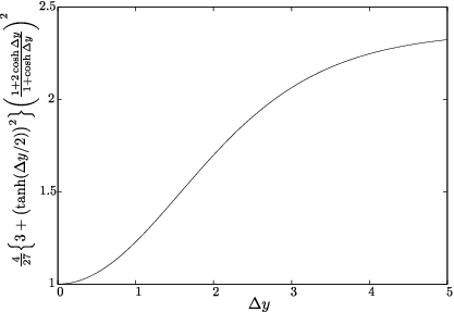
tr⁡[T⋅T†]=4​𝒌1⟂2​(𝒌~⟂⋅𝒌~⟂′)(𝒑⟂2)2⋅(1+2​cosh⁡Δ​y1+cosh⁡Δ​y)2.\mathrm{tr}[T\cdot T^{\dagger}]=\frac{4\boldsymbol{k}_{1\perp}^{2}(\widetilde{\boldsymbol{k}}_{\perp}\!\cdot\widetilde{\boldsymbol{k}}_{\perp}^{\prime})}{(\boldsymbol{p}_{\perp}^{2})^{2}}\cdot\biggl(\frac{1+2\cosh\Delta y}{1+\cosh\Delta y}\biggr)^{2}\,. (90)

Here we should not forget that 𝒌~⟂\widetilde{\boldsymbol{k}}_{\perp} and 𝒌~⟂′\widetilde{\boldsymbol{k}}_{\perp}^{\prime} have the rapidity dependence too. By shifting 𝒌⟂→𝒌⟂−𝒌1⟂/2\boldsymbol{k}_{\perp}\to\boldsymbol{k}_{\perp}-\boldsymbol{k}_{1\perp}/2 and 𝒌⟂′→𝒌⟂′−𝒌1⟂/2\boldsymbol{k}_{\perp}^{\prime}\to\boldsymbol{k}_{\perp}^{\prime}-\boldsymbol{k}_{1\perp}/2, the final expression for the back-to-back two-gluon production from the connected diagram is

⟨d​Ngd​|𝒑⟂|​d​|𝒒⟂|​d​θ​d​y1​d​y2|𝒒⟂=−𝒑⟂⟩conn=1π​Rp2​4​αs(Nc2−1)​(2​π)5​𝒑⟂2​∫d2​𝒌1⟂(2​π)2​φp​(𝒌1⟂)\displaystyle\biggl\langle\frac{\mathrm{d}N_{\text{g}}}{\mathrm{d}|\boldsymbol{p}_{\perp}|\mathrm{d}|\boldsymbol{q}_{\perp}|\mathrm{d}\theta\mathrm{d}y_{1}\mathrm{d}y_{2}}\biggr|_{\boldsymbol{q}_{\perp}=-\boldsymbol{p}_{\perp}}\biggr\rangle_{\text{conn}}\!\!\!=\frac{1}{\pi R_{\text{p}}^{2}}\frac{4\alpha_{\text{s}}}{(N_{\text{c}}^{2}\!-\!1)(2\pi)^{5}\boldsymbol{p}_{\perp}^{2}}\int\frac{\mathrm{d}^{2}\boldsymbol{k}_{1\perp}}{(2\pi)^{2}}\varphi_{\text{p}}(\boldsymbol{k}_{1\perp})
×∫d2​𝒌⟂(2​π)2​d2​𝒌⟂′(2​π)2​[𝒌⟂⋅𝒌⟂′+14​(tanh⁡(Δ​y/2))2​𝒌1⟂2]⋅(1+2​cosh⁡Δ​y1+cosh⁡Δ​y)2\displaystyle\times\int\frac{\mathrm{d}^{2}\boldsymbol{k}_{\perp}}{(2\pi)^{2}}\frac{\mathrm{d}^{2}\boldsymbol{k}^{\prime}_{\perp}}{(2\pi)^{2}}\Bigl[\boldsymbol{k}_{\perp}\!\cdot\boldsymbol{k}_{\perp}^{\prime}+\frac{1}{4}\bigl(\tanh(\Delta y/2)\bigr)^{2}\boldsymbol{k}_{1\perp}^{2}\Bigr]\cdot\biggl(\frac{1+2\cosh\Delta y}{1+\cosh\Delta y}\biggr)^{2} (91)
×⟨tr⁡[U⁡(𝒌⟂−𝒌1⟂/2)​TAa​U†​(𝒌⟂+𝒌1⟂/2)​U​(𝒌⟂′+𝒌1⟂/2)​TAa​U†​(𝒌⟂′−𝒌1⟂/2)]⟩,\displaystyle\times\bigl\langle\mathrm{tr}[U(\boldsymbol{k}_{\perp}\!\!-\!\boldsymbol{k}_{1\perp}\!/2)T_{\text{A}}^{a}U^{\dagger}(\boldsymbol{k}_{\perp}\!\!+\!\boldsymbol{k}_{1\perp}\!/2)\,U(\boldsymbol{k}_{\perp}^{\prime}\!\!+\!\boldsymbol{k}_{1\perp}\!/2)T_{\text{A}}^{a}U^{\dagger}(\boldsymbol{k}_{\perp}^{\prime}\!\!-\!\boldsymbol{k}_{1\perp}\!/2)]\bigr\rangle\,,

where θ\theta is the angle between 𝒒⟂\boldsymbol{q}_{\perp} and 𝒑⟂\boldsymbol{p}_{\perp}, and we have used the gluon distribution function defined in Eq. (95) in Appendix A. The transverse area π​Rp2\pi R_{\text{p}}^{2} originates from our definition of the gluon distribution function.

The expectation value of the Wilson line correlator includes contributions from all twists, which is numerically evaluated. If we make a leading twist approximation, we can analytically evaluate the Wilson line correlation, which is simply obtained as

⟨tr⁡[U⁡(𝒌⟂−𝒌1⟂/2)​TAa​U†​(𝒌⟂+𝒌1⟂/2)​U​(𝒌⟂′+𝒌1⟂/2)​TAa​U†​(𝒌⟂′−𝒌1⟂/2)]⟩\displaystyle\bigl\langle\mathrm{tr}[U(\boldsymbol{k}_{\perp}\!\!-\!\boldsymbol{k}_{1\perp}\!/2)T_{\text{A}}^{a}U^{\dagger}(\boldsymbol{k}_{\perp}\!\!+\!\boldsymbol{k}_{1\perp}\!/2)\,U(\boldsymbol{k}_{\perp}^{\prime}\!\!+\!\boldsymbol{k}_{1\perp}\!/2)T_{\text{A}}^{a}U^{\dagger}(\boldsymbol{k}_{\perp}^{\prime}\!\!-\!\boldsymbol{k}_{1\perp}\!/2)]\bigr\rangle\,
≈4​αs​φA​(𝒌1⟂)𝒌1⟂2​Nc2​(δ(2)​(𝒌⟂+𝒌1⟂2)​δ(2)​(𝒌⟂′+𝒌1⟂2)+δ(2)​(𝒌⟂−𝒌1⟂2)​δ(2)​(𝒌⟂′−𝒌1⟂2)CLOSE\displaystyle\approx\frac{4\alpha_{s}\varphi_{\text{A}}(\boldsymbol{k}_{1\perp})}{\boldsymbol{k}_{1\perp}^{2}}N_{\text{c}}^{2}\bigl(\delta^{(2)}(\boldsymbol{k}_{\perp}\!\!+\!\frac{\boldsymbol{k}_{1\perp}}{2})\delta^{(2)}(\boldsymbol{k}_{\perp}^{\prime}\!\!+\!\frac{\boldsymbol{k}_{1\perp}}{2})+\delta^{(2)}(\boldsymbol{k}_{\perp}\!\!-\!\frac{\boldsymbol{k}_{1\perp}}{2})\delta^{(2)}(\boldsymbol{k}_{\perp}^{\prime}\!\!-\!\frac{\boldsymbol{k}_{1\perp}}{2})
OPEN−12​δ(2)​(𝒌⟂+𝒌1⟂2)​δ(2)​(𝒌⟂′−𝒌1⟂2)−12​δ(2)​(𝒌⟂′+𝒌1⟂2)​δ(2)​(𝒌⟂−𝒌1⟂2)),\displaystyle\;\;\;\;-\frac{1}{2}\delta^{(2)}(\boldsymbol{k}_{\perp}\!\!+\!\frac{\boldsymbol{k}_{1\perp}}{2})\delta^{(2)}(\boldsymbol{k}_{\perp}^{\prime}\!\!-\!\frac{\boldsymbol{k}_{1\perp}}{2})-\frac{1}{2}\delta^{(2)}(\boldsymbol{k}_{\perp}^{\prime}\!\!+\!\frac{\boldsymbol{k}_{1\perp}}{2})\delta^{(2)}(\boldsymbol{k}_{\perp}\!\!-\!\frac{\boldsymbol{k}_{1\perp}}{2})\bigr)\;, (92)

where we have defined φA\varphi_{\text{A}} to mean the gluon distribution function of the nucleus. In this approximation, we obtain the correlation function as

⟨d​Ngd​|𝒑⟂|​d​|𝒒⟂|​d​θ​d​y1​d​y2|𝒒⟂=−𝒑⟂⟩conn=1π​Rp2​4​αs2​Nc2(Nc2−1)​(2​π)5​𝒑⟂2​∫d2​𝒌1⟂(2​π)2\displaystyle\biggl\langle\frac{\mathrm{d}N_{\text{g}}}{\mathrm{d}|\boldsymbol{p}_{\perp}|\mathrm{d}|\boldsymbol{q}_{\perp}|\mathrm{d}\theta\mathrm{d}y_{1}\mathrm{d}y_{2}}\biggr|_{\boldsymbol{q}_{\perp}=-\boldsymbol{p}_{\perp}}\biggr\rangle_{\text{conn}}\!\!\!=\frac{1}{\pi R_{\text{p}}^{2}}\frac{4\alpha_{s}^{2}N_{\text{c}}^{2}}{(N_{\text{c}}^{2}\!-\!1)(2\pi)^{5}\boldsymbol{p}_{\perp}^{2}}\int\frac{\mathrm{d}^{2}\boldsymbol{k}_{1\perp}}{(2\pi)^{2}}
×φp​(𝒌1⟂)​φA​(𝒌1⟂)​{3+(tanh⁡(Δ​y/2))2}​(1+2​cosh⁡Δ​y1+cosh⁡Δ​y)2.\displaystyle\qquad\times\varphi_{\text{p}}(\boldsymbol{k}_{1\perp})\,\varphi_{\text{A}}(\boldsymbol{k}_{1\perp})\Bigl\{3+\bigl(\tanh(\Delta y/2)\bigr)^{2}\Bigr\}\biggl(\frac{1+2\cosh\Delta y}{1+\cosh\Delta y}\biggr)^{2}\;. (93)

Although the expression in Eq. (93) has a k⟂k_{\perp}-factorized form, we cannot write the two-gluon production in general into such a k⟂k_{\perp}-factorized expression even in the pA case [9, 12]. In this back-to-back kinematics, the rapidity dependence is simply factorized as

⟨d​Ngd​|𝒑⟂|​d​|𝒒⟂|​d​θ​d​y1​d​y2|𝒒⟂=−𝒑⟂⟩conn=⟨d​Nggd​|𝒑⟂|​d​|𝒒⟂|​d​θ​d​y1​d​y2|𝒒⟂=−𝒑⟂,Δ​y=0⟩conn\displaystyle\biggl\langle\frac{\mathrm{d}N_{\text{g}}}{\mathrm{d}|\boldsymbol{p}_{\perp}|\mathrm{d}|\boldsymbol{q}_{\perp}|\mathrm{d}\theta\mathrm{d}y_{1}\mathrm{d}y_{2}}\biggr|_{\boldsymbol{q}_{\perp}=-\boldsymbol{p}_{\perp}}\biggr\rangle_{\text{conn}}\!\!\!=\biggl\langle\frac{\mathrm{d}N_{\text{gg}}}{\mathrm{d}|\boldsymbol{p}_{\perp}|\mathrm{d}|\boldsymbol{q}_{\perp}|\mathrm{d}\theta\mathrm{d}y_{1}\mathrm{d}y_{2}}\biggr|_{\boldsymbol{q}_{\perp}=-\boldsymbol{p}_{\perp},\Delta y=0}\biggr\rangle_{\text{conn}}
×427​{3+(tanh⁡(Δ​y/2))2}​(1+2​cosh⁡Δ​y1+cosh⁡Δ​y)2.\displaystyle\qquad\qquad\qquad\times\frac{4}{27}\Bigl\{3+\bigl(\tanh(\Delta y/2)\bigr)^{2}\Bigr\}\biggl(\frac{1+2\cosh\Delta y}{1+\cosh\Delta y}\biggr)^{2}\;. (94)

The correlation function is a monotonously increasing function of Δ​y\Delta y. In Fig. 5, we show the rapidity correlation associated with the two-gluon production in the back-to-back case. It is remarkable that the correlation is enhanced as the rapidity difference increases, which is valid as long as Δ​y<1/αs\Delta y<1/\alpha_{\text{s}}. At asymptotically large rapidity difference with Δ​y→∞\Delta y\to\infty, if the quantum evolution between Δ​y\Delta y is neglected, the correlation function exactly reproduces the result in the eikonal limit, which is in agreement with Ref. [5].

Refer to caption
Figure 5: Dependence on Δ​y\Delta y in the leading-twist approximation.

6 Conclusions

We explicitly calculated the two-gluon correlation in the pA collision using the framework of the Color Glass Condensate and the LSZ reduction formula. We specifically chose a connected diagram, which is the leading order of the coupling gg and the weak color source, and could be the only contribution to produce the intrinsic dependence on the longitudinal or rapidity separation between emitted gluons. To accomplish the calculation we wrote down the classical gluon field associated with the dilute and dense color sources and put it to the background propagator.

Our final results encompass the rapidity dependence that is not taken into account in the eikonal limit, but they are too complicated to perceive the qualitative behavior as a function of the rapidity separation. We have to wait for numerical evaluation, which we plan to do as a natural extension of this work, in order to extract phenomenological physics implication from our analytical expressions.

In this paper we proceeded to analyzing the rapidity dependence in the special cases. First, we confirmed that our expressions are certainly reduced to the known expression given in Ref. [10] in the eikonal limit. Next, we relaxed this limit so as to allow for the rapidity separation under the condition that the momenta carried by emitted gluons are hard as compared to the gluon distribution in the projectile and target hadrons. In this case we found a fairly concise formula for the two-gluon production in the back-to-back kinematics. Our results imply that the dependence on the rapidity separation is only moderate and there arise no exponentially damping correlations.

In fact, our finding is the other way around; the connected diagram enhances the long-range correlations in rapidity. That is, the contribution to the multiplicity from the connected diagram gets larger with increasing rapidity separation. Although this might sound curious at first, this could be possible because we consider two gluons split from one gluon. The long-range correlations in this case simply signifies that more gluons come out with larger longitudinal angle. In fact, the three-point vertex in QCD contains p+/q+=eΔ​yp^{+}/q^{+}=\mathrm{e}^{\Delta y} which surpasses the energy denominator. We remind that our tree-level description breaks down eventually for Δ​y>1/αs\Delta y>1/\alpha_{\text{s}} due to quantum effects.

It is quite interesting to see such long-range correlations in rapidity and this observation seems to be consistent with the ridge phenomenon observed at RHIC [27, 28, 29]. We cannot, of course, make any convincing statement about the near-side jet correlations from our rough analyses limited to the back-to-back kinetics. It is indispensable to perform the numerical integration to quantify the two-gluon production. In the near future we are planning to include the disconnected diagram, which is much simpler than the connected one we manipulated here, to discuss not only the rapidity dependence but also the azimuthal angle dependence and their interplay in this framework [42].

We thank Larry McLerran for encouraging us to initiate this problem. We thank François Gelis and Raju Venugopalan for discussions. We also thank François Fillion-Gourdeau for useful comments. K. F. is supported by Japanese MEXT grant No. 20740134 and also supported in part by Yukawa International Program for Quark Hadron Sciences (YIPQS). This research is supported in part by RIKEN BNL Research Center and the US Department of Energy under cooperative research agreement #DE-AC02-98CH10886.

Appendix A Appendix – Gluon Distributions

To make the final expression (78) more comprehensible in an intuitive way let us make use of the notation by the parton distribution functions along the similar line as Ref. [9]. We first define the proton unintegrated gluon distribution;

⟨ρpa(𝒌1⟂)ρpa′∗(𝒌1⟂′)⟩=δa​a′​𝒌1⟂2π⁡(Nc2−1)​∫d2​𝑿⟂​ei⁡(𝒌1⟂−𝒌1⟂′)⋅𝑿⟂​d​φp​(𝒌1⟂|𝑿⟂)d2​𝑿⟂,\begin{split}&\bigl\langle\rho_{\text{p}}^{a}(\boldsymbol{k}_{1\perp})\rho_{\text{p}}^{a^{\prime}\ast}(\boldsymbol{k}_{1\perp}^{\prime})\bigr\rangle\\ &=\frac{\delta^{aa^{\prime}}\,\boldsymbol{k}_{1\perp}^{2}}{\pi(N_{\text{c}}^{2}-1)}\int\mathrm{d}^{2}\boldsymbol{X}_{\perp}\,\mathrm{e}^{\mathrm{i}(\boldsymbol{k}_{1\perp}\!-\boldsymbol{k}_{1\perp}^{\prime})\cdot\boldsymbol{X}_{\perp}}\frac{\mathrm{d}\varphi_{\text{p}}\bigl(\boldsymbol{k}_{1\perp}\big|\boldsymbol{X}_{\perp}\!\bigr)}{\mathrm{d}^{2}\boldsymbol{X}_{\perp}}\,,\end{split} (95)

where we have assumed 𝒌1⟂≈𝒌1⟂′\boldsymbol{k}_{1\perp}\approx\boldsymbol{k}_{1\perp}^{\prime}. The above equality could be understood as the definition for φp​(𝒌⟂|𝑿⟂)\varphi_{\text{p}}(\boldsymbol{k}_{\perp}|\boldsymbol{X}_{\perp}). It is a straightforward generalization to proceed to the definition for the two-point correlator, that is,

δa​a′​⟨Ub​a​(𝒌2⟂)​U†a′​b′​(𝒌2⟂′)​tr​[TAb​TAb′]⟩=Nc​⟨tr⁡[U⁡(𝒌2⟂)​U†​(𝒌2⟂′)]⟩=g2​Nc2π​𝒌2⟂2​∫d2​𝑿⟂​ei⁡(𝒌2⟂−𝒌2⟂′)⋅𝑿⟂​d​φAg,g​(𝒌2⟂|𝑿⟂−𝒃)d2​𝑿⟂.\begin{split}&\delta^{aa^{\prime}}\bigl\langle U^{ba}(\boldsymbol{k}_{2\perp})\,U^{\dagger a^{\prime}b^{\prime}}(\boldsymbol{k}_{2\perp}^{\prime})\mathrm{tr}[T_{\text{A}}^{b}T_{\text{A}}^{b^{\prime}}]\bigr\rangle=N_{\text{c}}\bigl\langle\mathrm{tr}\bigl[U(\boldsymbol{k}_{2\perp})\,U^{\dagger}(\boldsymbol{k}_{2\perp}^{\prime})\bigr]\bigr\rangle\\ &=\frac{g^{2}N_{\text{c}}^{2}}{\pi\boldsymbol{k}_{2\perp}^{2}}\int\mathrm{d}^{2}\boldsymbol{X}_{\perp}\,\mathrm{e}^{i(\boldsymbol{k}_{2\perp}\!-\boldsymbol{k}_{2\perp}^{\prime})\cdot\boldsymbol{X}_{\perp}}\,\frac{\mathrm{d}\varphi^{g,g}_{A}(\boldsymbol{k}_{2\perp}|\boldsymbol{X}_{\perp}\!-\boldsymbol{b})}{\mathrm{d}^{2}\boldsymbol{X}_{\perp}}\,.\end{split} (96)

We should note that 𝒃\boldsymbol{b} is the impact parameter that specifies the relative separation from the proton gluon distribution in the transverse plane. The three-point correlator goes on to be

δa​a′​⟨tr⁡[U⁡(𝒌⟂)​TAa​U†​(𝒌⟂−𝒌2⟂)​TAb′]​U†a′​b′​(𝒌2⟂′)⟩=g2​Nc2π​𝒌2⟂2​∫d2​𝑿⟂​ei⁡(𝒌2⟂−𝒌2⟂′)⋅𝑿⟂​d​φAg​g,g​(𝒌⟂,𝒌2⟂−𝒌⟂;𝒌2⟂|𝑿⟂−𝒃)d2​𝑿⟂.\begin{split}&\delta^{aa^{\prime}}\bigl\langle\mathrm{tr}\bigl[U(\boldsymbol{k}_{\perp})T_{\text{A}}^{a}U^{\dagger}(\boldsymbol{k}_{\perp}\!-\boldsymbol{k}_{2\perp})T_{\text{A}}^{b^{\prime}}\bigr]U^{\dagger a^{\prime}b^{\prime}}(\boldsymbol{k}_{2\perp}^{\prime})\bigr\rangle\\ &=\frac{g^{2}N_{\text{c}}^{2}}{\pi\boldsymbol{k}_{2\perp}^{2}}\int\mathrm{d}^{2}\boldsymbol{X}_{\perp}\,\mathrm{e}^{i(\boldsymbol{k}_{2\perp}\!-\boldsymbol{k}_{2\perp}^{\prime})\cdot\boldsymbol{X}_{\perp}}\frac{\mathrm{d}\varphi^{gg,g}_{A}(\boldsymbol{k}_{\perp},\boldsymbol{k}_{2\perp}\!-\boldsymbol{k}_{\perp};\boldsymbol{k}_{2\perp}|\boldsymbol{X}_{\perp}\!-\boldsymbol{b})}{\mathrm{d}^{2}\boldsymbol{X}_{\perp}}\,.\end{split} (97)

The four-point correlator is

δa​a′​⟨tr⁡[U⁡(𝒌⟂)​TAa​U†​(𝒌⟂−𝒌2⟂)​U​(𝒌⟂′−𝒌2⟂′)​TAa′​U†​(𝒌⟂′)]⟩=g2​Nc2π​𝒌2⟂2​∫d2​𝑿⟂​ei⁡(𝒌2⟂−𝒌2⟂′)⋅𝑿⟂​d​φAg​g,g​g​(𝒌⟂,𝒌2⟂−𝒌⟂;𝒌⟂′,𝒌2⟂−𝒌⟂′|𝑿⟂−𝒃)d2​𝑿⟂.\begin{split}&\delta^{aa^{\prime}}\bigl\langle\mathrm{tr}\bigl[U(\boldsymbol{k}_{\perp})T_{\text{A}}^{a}U^{\dagger}(\boldsymbol{k}_{\perp}\!-\boldsymbol{k}_{2\perp})U(\boldsymbol{k}_{\perp}^{\prime}\!-\boldsymbol{k}_{2\perp}^{\prime})T_{\text{A}}^{a^{\prime}}U^{\dagger}(\boldsymbol{k}_{\perp}^{\prime})\bigr]\bigr\rangle\\ &=\frac{g^{2}N_{\text{c}}^{2}}{\pi\boldsymbol{k}_{2\perp}^{2}}\int\mathrm{d}^{2}\boldsymbol{X}_{\perp}\,\mathrm{e}^{i(\boldsymbol{k}_{2\perp}\!-\boldsymbol{k}_{2\perp}^{\prime})\cdot\boldsymbol{X}_{\perp}}\frac{\mathrm{d}\varphi^{gg,gg}_{A}(\boldsymbol{k}_{\perp},\boldsymbol{k}_{2\perp}\!-\boldsymbol{k}_{\perp};\boldsymbol{k}_{\perp}^{\prime},\boldsymbol{k}_{2\perp}\!-\boldsymbol{k}_{\perp}^{\prime}|\boldsymbol{X}_{\perp}-\boldsymbol{b})}{\mathrm{d}^{2}\boldsymbol{X}_{\perp}}\,.\end{split} (98)

Here we assume that the distribution functions are approximately homogeneous in transverse space, which is often the case in the McLerran-Venugopalan model treatment based on the Gaussian distribution for the color source. Then, the integration over the transverse plane gives rise to the momentum delta functions, which simplifies the final results to be

⟨d​Ngd​y1​d​y2⟩conn=1π​Rp2​αs2​Nc2(Nc2−1)​π2​∫d2​𝒑⟂(2​π)2​d2​𝒒⟂(2​π)2​d2​𝒌1⟂(2​π)2​φp​(𝒌1⟂)𝒌1⟂2​𝒌2⟂2\displaystyle\biggl\langle\frac{\mathrm{d}N_{\text{g}}}{\mathrm{d}y_{1}\mathrm{d}y_{2}}\biggr\rangle_{\text{conn}}\!\!\!=\frac{1}{\pi R_{\text{p}}^{2}}\frac{\alpha^{2}_{s}N_{\text{c}}^{2}}{(N_{\text{c}}^{2}-1)\pi^{2}}\int\frac{\mathrm{d}^{2}\boldsymbol{p}_{\perp}}{(2\pi)^{2}}\frac{\mathrm{d}^{2}\boldsymbol{q}_{\perp}}{(2\pi)^{2}}\frac{\mathrm{d}^{2}\boldsymbol{k}_{1\perp}}{(2\pi)^{2}}\;\frac{\varphi_{\text{p}}(\boldsymbol{k}_{1\perp})}{\boldsymbol{k}_{1\perp}^{2}\boldsymbol{k}_{2\perp}^{2}}
×{tr[T(>)⋅T(>)†]φAg,g(𝒌2⟂)+∫d2​𝒌⟂(2​π)2tr[T(<)⋅T(>)†]φAg​g,g(𝒌⟂,𝒌2⟂−𝒌⟂;𝒌2⟂)\displaystyle\times\biggl\{\mathrm{tr}[T_{(>)}\cdot T_{(>)}^{\dagger}]\,\varphi^{g,g}_{A}(\boldsymbol{k}_{2\perp})+\int\frac{\mathrm{d}^{2}\boldsymbol{k}_{\perp}}{(2\pi)^{2}}\,\mathrm{tr}[T_{(<)}\cdot T_{(>)}^{\dagger}]\,\varphi^{gg,g}_{A}(\boldsymbol{k}_{\perp},\boldsymbol{k}_{2\perp}\!-\boldsymbol{k}_{\perp};\boldsymbol{k}_{2\perp})
+∫d2​𝒌⟂′(2​π)2tr[T(>)⋅T(<)†]φAg​g,g(𝒌⟂,𝒌2⟂−𝒌⟂;𝒌2⟂)\displaystyle\qquad+\int\frac{\mathrm{d}^{2}\boldsymbol{k}^{\prime}_{\perp}}{(2\pi)^{2}}\,\mathrm{tr}[T_{(>)}\cdot T_{(<)}^{\dagger}]\,\varphi^{gg,g}_{A}(\boldsymbol{k}_{\perp},\boldsymbol{k}_{2\perp}\!-\boldsymbol{k}_{\perp};\boldsymbol{k}_{2\perp}) (99)
+∫d2​𝒌⟂(2​π)2d2​𝒌⟂′(2​π)2tr[T(<)⋅T(<)†]φAg​g,g​g(𝒌⟂,𝒌2⟂−𝒌⟂;𝒌⟂′,𝒌2⟂−𝒌⟂′)},\displaystyle\qquad+\int\frac{\mathrm{d}^{2}\boldsymbol{k}_{\perp}}{(2\pi)^{2}}\frac{\mathrm{d}^{2}\boldsymbol{k}^{\prime}_{\perp}}{(2\pi)^{2}}\,\mathrm{tr}[T_{(<)}\cdot T_{(<)}^{\dagger}]\,\varphi^{gg,gg}_{A}(\boldsymbol{k}_{\perp},\boldsymbol{k}_{2\perp}\!-\boldsymbol{k}_{\perp};\boldsymbol{k}_{\perp}^{\prime},\boldsymbol{k}_{2\perp}\!-\boldsymbol{k}_{\perp}^{\prime})\biggr\}\,,

where RpR_{\text{p}} is the transverse radius of the proton. It is necessary to calculate the gluon distribution functions for numerical evaluation and we can utilize the McLerran-Venugopalan model. Appendix B is devoted to the explanation of how to compute the average of the Wilson lines.

Appendix B Appendix – Average of the Wilson Lines

In this appendix, we evaluate the Gaussian average for the two-, three- and four-point functions in terms of the Wilson line in the adjoint representation. They are all necessary to compute the gluon distribution functions in the McLerran-Venugopalan model. For this purpose it is enough to calculate the four-point function because the two- and three-point functions are readily deduced by the appropriate contraction from the four-point function as

Nc​⟨tr⁡[U⁡(𝒙1⟂)​U†​(𝒙2⟂)]⟩=⟨tr⁡[U⁡(𝒙1⟂)​TAa​U†​(𝒙3⟂)​U​(𝒙3⟂)​TAa​U†​(𝒙2⟂)]⟩,N_{\text{c}}\bigl\langle\mathrm{tr}[U(\boldsymbol{x}_{1\perp})U^{\dagger}(\boldsymbol{x}_{2\perp})]\bigr\rangle=\bigl\langle\mathrm{tr}[U(\boldsymbol{x}_{1\perp})T_{\text{A}}^{a}U^{\dagger}(\boldsymbol{x}_{3\perp})U(\boldsymbol{x}_{3\perp})T_{\text{A}}^{a}U^{\dagger}(\boldsymbol{x}_{2\perp})]\bigr\rangle\,, (100)

and

⟨tr⁡[U⁡(𝒙1⟂)​TAa​U†​(𝒙2⟂)​TAb]​U†a​b​(𝒙3⟂)⟩=⟨tr⁡[U⁡(𝒙1⟂)​TAa​U†​(𝒙2⟂)​U​(𝒙3⟂)​TAa​U†​(𝒙3⟂)]⟩.\begin{split}&\bigl\langle\mathrm{tr}[U(\boldsymbol{x}_{1\perp})T_{\text{A}}^{a}U^{\dagger}(\boldsymbol{x}_{2\perp})T_{\text{A}}^{b}]U^{\dagger ab}(\boldsymbol{x}_{3\perp})\bigr\rangle\\ &\qquad=\bigl\langle\mathrm{tr}[U(\boldsymbol{x}_{1\perp})T_{\text{A}}^{a}U^{\dagger}(\boldsymbol{x}_{2\perp})U(\boldsymbol{x}_{3\perp})T_{\text{A}}^{a}U^{\dagger}(\boldsymbol{x}_{3\perp})]\bigr\rangle\,.\end{split} (101)

Calculating the generic four-point function in the adjoint representation is a tedious task, though it is not impossible. Instead, we thus adopt the large-NcN_{\text{c}} expansion here. We can express the adjoint Wilson line using the fundamental Wilson lines as

U​(𝒙i⟂)β​α=2​tr​[TFβ​UF​(𝒙i⟂)​TFα​UF†​(𝒙i⟂)],U(\boldsymbol{x}_{i\perp})_{\beta\alpha}=2\mathrm{tr}[T_{\text{F}}^{\beta}U_{\text{F}}(\boldsymbol{x}_{i\perp})T_{\text{F}}^{\alpha}U_{\text{F}}^{\dagger}(\boldsymbol{x}_{i\perp})]\,, (102)

where UF​(𝒙i⟂)U_{\text{F}}(\boldsymbol{x}_{i\perp}) is the fundamental Wilson line and TFT_{\text{F}} is the generator in the fundamental representation. Using Eq. (102) we can then rewrite the four-point function in the adjoint representation as follows;

⟨tr⁡[U⁡(𝒙1⟂)​TAa​U†​(𝒙2⟂)​U​(𝒙3⟂)​TAa​U†​(𝒙4⟂)]⟩\displaystyle\bigl\langle\mathrm{tr}[U(\boldsymbol{x}_{1\perp})T_{\text{A}}^{a}U^{\dagger}(\boldsymbol{x}_{2\perp})U(\boldsymbol{x}_{3\perp})T_{\text{A}}^{a}U^{\dagger}(\boldsymbol{x}_{4\perp})]\bigr\rangle
=4​TAaα1​α2​TAaα3​α4​TFα1a1​a¯1​TFα2a2​a¯2​TFα3a3​a¯3​TFα4a4​a¯4\displaystyle=4{T_{\text{A}}^{a}}_{\alpha_{1}\alpha_{2}}{T_{\text{A}}^{a}}_{\alpha_{3}\alpha_{4}}{T_{\text{F}}^{\alpha_{1}}}_{a_{1}\bar{a}_{1}}{T_{\text{F}}^{\alpha_{2}}}_{a_{2}\bar{a}_{2}}{T_{\text{F}}^{\alpha_{3}}}_{a_{3}\bar{a}_{3}}{T_{\text{F}}^{\alpha_{4}}}_{a_{4}\bar{a}_{4}} (103)
×4​δβ1​β4​δβ2​β3​TFβ1b¯1​b1​TFβ2b¯2​b2​TFβ3b¯3​b3​TFβ4b¯4​b4​⟨∏i=14UF​bi​ai​(𝒙i⟂)​UF​b¯i​a¯i∗​(𝒙i⟂)⟩.\displaystyle\quad\times 4\delta_{\beta_{1}\beta_{4}}\delta_{\beta_{2}\beta_{3}}{T_{\text{F}}^{\beta_{1}}}_{\bar{b}_{1}b_{1}}{T_{\text{F}}^{\beta_{2}}}_{\bar{b}_{2}b_{2}}{T_{\text{F}}^{\beta_{3}}}_{\bar{b}_{3}b_{3}}{T_{\text{F}}^{\beta_{4}}}_{\bar{b}_{4}b_{4}}\bigl\langle\prod_{i=1}^{4}U_{\text{F}b_{i}a_{i}}(\boldsymbol{x}_{i\perp})U^{\ast}_{\text{F}\bar{b}_{i}\bar{a}_{i}}(\boldsymbol{x}_{i\perp})\bigr\rangle\,.

In the same way as the present authors did in Ref. [45] we shall introduce the “initial state” and the “finial state” as

⟨a1,a2,a3,a4,a¯1,a¯2,a¯3,a¯4|initial⟩=4TAaα1​α2TAaα3​α4TFα1a1​a¯1TFα2a2​a¯2TFα3a3​a¯3TFα4a4​a¯4\displaystyle\langle a_{1},a_{2},a_{3},a_{4},\bar{a}_{1},\bar{a}_{2},\bar{a}_{3},\bar{a}_{4}|\text{initial}\rangle=4{T_{\text{A}}^{a}}_{\alpha_{1}\alpha_{2}}{T_{\text{A}}^{a}}_{\alpha_{3}\alpha_{4}}{T_{\text{F}}^{\alpha_{1}}}_{a_{1}\bar{a}_{1}}{T_{\text{F}}^{\alpha_{2}}}_{a_{2}\bar{a}_{2}}{T_{\text{F}}^{\alpha_{3}}}_{a_{3}\bar{a}_{3}}{T_{\text{F}}^{\alpha_{4}}}_{a_{4}\bar{a}_{4}}
=12​(δa1​a¯4​δa2​a¯1​δa3​a¯2​δa4​a¯3+δa1​a¯2​δa2​a¯3​δa3​a¯4​δa4​a¯1CLOSE\displaystyle=\frac{1}{2}\bigl(\delta_{a_{1}\bar{a}_{4}}\delta_{a_{2}\bar{a}_{1}}\delta_{a_{3}\bar{a}_{2}}\delta_{a_{4}\bar{a}_{3}}+\delta_{a_{1}\bar{a}_{2}}\delta_{a_{2}\bar{a}_{3}}\delta_{a_{3}\bar{a}_{4}}\delta_{a_{4}\bar{a}_{1}}
OPEN−δa1​a¯3​δa2​a¯1​δa3​a¯4​δa4​a¯2−δa1​a¯2​δa2​a¯4​δa3​a¯1​δa4​a¯3),\displaystyle\qquad\qquad-\delta_{a_{1}\bar{a}_{3}}\delta_{a_{2}\bar{a}_{1}}\delta_{a_{3}\bar{a}_{4}}\delta_{a_{4}\bar{a}_{2}}-\delta_{a_{1}\bar{a}_{2}}\delta_{a_{2}\bar{a}_{4}}\delta_{a_{3}\bar{a}_{1}}\delta_{a_{4}\bar{a}_{3}}\bigr)\,, (104)
⟨final|b1,b2,b3,b4,b¯1,b¯2,b¯3,b¯4⟩=4δβ1​β4δβ2​β3TFβ1b¯1​b1TFβ2b¯2​b2TFβ3b¯3​b3TFβ4b¯4​b4\displaystyle\langle\text{final}|b_{1},b_{2},b_{3},b_{4},\bar{b}_{1},\bar{b}_{2},\bar{b}_{3},\bar{b}_{4}\rangle=4\delta_{\beta_{1}\beta_{4}}\delta_{\beta_{2}\beta_{3}}{T_{\text{F}}^{\beta_{1}}}_{\bar{b}_{1}b_{1}}{T_{\text{F}}^{\beta_{2}}}_{\bar{b}_{2}b_{2}}{T_{\text{F}}^{\beta_{3}}}_{\bar{b}_{3}b_{3}}{T_{\text{F}}^{\beta_{4}}}_{\bar{b}_{4}b_{4}}
=δb1​b¯4​δb2​b¯3​δb3​b¯2​δb4​b¯1+1Nc2​δb1​b¯1​δb2​b¯2​δb3​b¯3​δb4​b¯4\displaystyle=\delta_{b_{1}\bar{b}_{4}}\delta_{b_{2}\bar{b}_{3}}\delta_{b_{3}\bar{b}_{2}}\delta_{b_{4}\bar{b}_{1}}+\frac{1}{N_{\text{c}}^{2}}\delta_{b_{1}\bar{b}_{1}}\delta_{b_{2}\bar{b}_{2}}\delta_{b_{3}\bar{b}_{3}}\delta_{b_{4}\bar{b}_{4}}
−1Nc​(δb1​b¯1​δb2​b¯3​δb3​b¯2​δb4​b¯4+δb1​b¯4​δb2​b¯2​δb3​b¯3​δb4​b¯1),\displaystyle\qquad\qquad-\frac{1}{N_{\text{c}}}\bigl(\delta_{b_{1}\bar{b}_{1}}\delta_{b_{2}\bar{b}_{3}}\delta_{b_{3}\bar{b}_{2}}\delta_{b_{4}\bar{b}_{4}}+\delta_{b_{1}\bar{b}_{4}}\delta_{b_{2}\bar{b}_{2}}\delta_{b_{3}\bar{b}_{3}}\delta_{b_{4}\bar{b}_{1}}\bigr)\,, (105)

and also define the “Hamiltonian” composed of the free part, H0H_{0}, and the interaction VV;

H0\displaystyle H_{0} =Qs′2NcL(0,0)[∑i=14(TFia−TFi¯a∗)]2,\displaystyle=\frac{Q_{\text{s}}^{\prime 2}}{N_{\text{c}}}L(0,0)\biggl[\sum_{i=1}^{4}({T_{\text{F}}}_{i}^{a}-{T_{\text{F}}}_{\bar{i}}^{a\ast})\biggr]^{2}\,, (106)
V\displaystyle V =−Qs′2Nc{∑i>j4[TFiaTFjaΓ(𝒙i⟂,𝒙j⟂)+TFi¯a∗TFj¯a∗Γ(𝒙i⟂,𝒙j⟂)]\displaystyle=-\frac{Q_{\text{s}}^{\prime 2}}{N_{\text{c}}}\biggl\{\sum_{i>j}^{4}\bigl[{T_{\text{F}}}^{a}_{i}\,{T_{\text{F}}}^{a}_{j}\,\varGamma(\boldsymbol{x}_{i\perp},\boldsymbol{x}_{j\perp})+{T_{\text{F}}}^{a\ast}_{\bar{i}}\,{T_{\text{F}}}^{a\ast}_{\bar{j}}\,\varGamma(\boldsymbol{x}_{i\perp},\boldsymbol{x}_{j\perp})\bigr]
−∑i,j=14TFiaTFj¯a∗Γ(𝒙i⟂,𝒙j⟂)},\displaystyle\qquad-\sum_{i,j=1}^{4}{T_{\text{F}}}^{a}_{i}\,{T_{\text{F}}}^{a\ast}_{\bar{j}}\,\varGamma(\boldsymbol{x}_{i\perp},\boldsymbol{x}_{j\perp})\biggr\}\,, (107)

where we use the same notation as in Ref. [45] as

L⁡(𝒙1⟂,𝒙2⟂)=g4​∫d2​𝒛⟂​G0​(𝒙1⟂−𝒛⟂)​G0​(𝒙2⟂−𝒛⟂),Γ⁡(𝒙1⟂,𝒙2⟂)=2​L​(0,0)−2​L​(𝒙1⟂,𝒙2⟂).\begin{split}L(\boldsymbol{x}_{1\perp},\boldsymbol{x}_{2\perp})&=g^{4}\int\mathrm{d}^{2}\boldsymbol{z}_{\perp}\,G_{0}(\boldsymbol{x}_{1\perp}\!-\!\boldsymbol{z}_{\perp})\,G_{0}(\boldsymbol{x}_{2\perp}\!-\!\boldsymbol{z}_{\perp})\,,\\ \varGamma(\boldsymbol{x}_{1\perp},\boldsymbol{x}_{2\perp})&=2L(0,0)-2L(\boldsymbol{x}_{1\perp},\boldsymbol{x}_{2\perp})\,.\end{split} (108)

Here G0​(𝒙⟂−𝒛⟂)G_{0}(\boldsymbol{x}_{\perp}\!-\!\boldsymbol{z}_{\perp}) is the propagator in two dimensions satisfying ∂⟂2G0​(𝒙⟂−𝒛⟂)=δ(2)​(𝒙⟂−𝒛⟂)\partial_{\perp}^{2}G_{0}(\boldsymbol{x}_{\perp}\!-\!\boldsymbol{z}_{\perp})=\delta^{(2)}(\boldsymbol{x}_{\perp}-\boldsymbol{z}_{\perp}). We note that the saturation scale Qs′Q_{\text{s}}^{\prime} has a different normalization from Ref. [45], that is, we have defined Qs′2=2​Nc2/(Nc2−1)​Qs2Q_{\text{s}}^{\prime 2}=2N_{\text{c}}^{2}/(N_{\text{c}}^{2}-1)Q_{\text{s}}^{2}. By means of the bra- and ket-vectors, the initial and final states become

|initial⟩=12​Nc2​(|4123⟩+|2341⟩−|3142⟩−|2413⟩),⟨final|=Nc2​⟨4321|+⟨1234|−Nc​⟨1324|−Nc​⟨4231|,\begin{split}|\text{initial}\rangle&=\frac{1}{2}N_{\text{c}}^{2}\bigl(|4123\rangle+|2341\rangle-|3142\rangle-|2413\rangle\bigr)\,,\\ \langle\text{final}|&=N_{\text{c}}^{2}\langle\text{4321}|+\langle\text{1234}|-N_{\text{c}}\langle\text{1324}|-N_{\text{c}}\langle\text{4231}|\,,\end{split}

where we define

⟨a1,a2,a3,a4,a¯1,a¯2,a¯3,a¯4|ijkl⟩=1Nc2δa1​a¯iδa2​a¯jδa3​a¯kδa4​a¯l,\langle a_{1},a_{2},a_{3},a_{4},\bar{a}_{1},\bar{a}_{2},\bar{a}_{3},\bar{a}_{4}|ijkl\rangle=\frac{1}{N_{\text{c}}^{2}}\delta_{a_{1}\bar{a}_{i}}\delta_{a_{2}\bar{a}_{j}}\delta_{a_{3}\bar{a}_{k}}\delta_{a_{4}\bar{a}_{l}}\,, (109)

whose norm is normalized properly to unity. Here we note that |i​j​k​l⟩|ijkl\rangle’s form a complete set of the singlet states out of Nc⊗Nc∗⊗Nc⊗Nc∗⊗Nc⊗Nc∗⊗Nc⊗Nc∗N_{\text{c}}\otimes N_{\text{c}}^{*}\otimes N_{\text{c}}\otimes N_{\text{c}}^{*}\otimes N_{\text{c}}\otimes N_{\text{c}}^{*}\otimes N_{\text{c}}\otimes N_{\text{c}}^{*}, that is, satisfy H0​|i​j​k​l⟩=0H_{0}|ijkl\rangle=0, though |i​j​k​l⟩|ijkl\rangle is not the orthogonal basis.

Let us consider the large-NcN_{\text{c}} limit and then one might naively think that the leading order of the matrix element would be 𝒪⁡(Nc4)\mathcal{O}(N_{\text{c}}^{4}) since both the initial and final states are 𝒪⁡(Nc2)\mathcal{O}(N_{\text{c}}^{2}). This is, however, not true. In the large-NcN_{\text{c}} limit VV is diagonal and ⟨final|initial⟩=𝒪⁡(Nc3)\langle\text{final}|\text{initial}\rangle=\mathcal{O}(N_{\text{c}}^{3}) [14, 45]. Unfortunately, since the leading-order contribution vanishes, we need to calculate the next-to-leading order in the large NcN_{\text{c}} expansion.

For the purpose of proceeding to the next-to-leading order, we need to know the overlap between different states. These are directly read as

⟨4321|4123⟩=⟨4321|2341⟩=1Nc,⟨4321|3142⟩=⟨4321|2413⟩=1Nc2.\begin{split}\langle 4321|4123\rangle&=\langle 4321|2341\rangle=\frac{1}{N_{\text{c}}}\,,\\ \langle 4321|3142\rangle&=\langle 4321|2413\rangle=\frac{1}{N_{\text{c}}^{2}}\,.\end{split} (110)

As we mentioned above, the matrix elements of e−V\mathrm{e}^{-V} are 𝒪⁡(1)\mathcal{O}(1) for the (vanishing) diagonal components and are 𝒪⁡(1/Nc)\mathcal{O}(1/N_{\text{c}}) for the off-diagonal components. Hence the only first equation in Eq. (110) gives a finite contribution to the next-to-leading order, while the second one is the next-to-next-to-leading order in this counting.

As a result of the truncation up to 𝒪⁡(Nc3)\mathcal{O}(N_{\text{c}}^{3}) the matrix element is expressed as

⟨final|e−V|initial⟩≃Nc42​(⟨4321|e−V|4123⟩+⟨4321​|e−V|​2341⟩).\langle\text{final}|\mathrm{e}^{-V}|\text{initial}\rangle\simeq\frac{N_{\text{c}}^{4}}{2}\bigl(\langle 4321|\mathrm{e}^{-V}|4123\rangle+\langle 4321|\mathrm{e}^{-V}|2341\rangle\bigr)\,. (111)

Henceforth, let us focus on the evaluation of ⟨4321|e−V|4123⟩\langle 4321|\mathrm{e}^{-V}|4123\rangle appearing in Eq. (111). By definition e−V\mathrm{e}^{-V} is expanded as

e−V=∑n=0∞(−1)nn!​Vn.\mathrm{e}^{-V}=\sum_{n=0}^{\infty}\frac{(-1)^{n}}{n!}V^{n}\,. (112)

We shall operate VV onto |4123⟩|4123\rangle and |4321⟩|4321\rangle. Using the diagrammatical technique developed in Ref. [45] we can find,

V​|4123⟩=V11​|4123⟩+1Nc​V21​|4321⟩+⋯,V​|4321⟩=V22​|4321⟩+⋯,\begin{split}V|4123\rangle&=V_{11}|4123\rangle+\frac{1}{N_{\text{c}}}V_{21}|4321\rangle+\cdots\,,\\ V|4321\rangle&=V_{22}|4321\rangle+\cdots\,,\end{split} (113)

where

V11\displaystyle V_{11} =Qs′22​[Γ⁡(𝒙1⟂,𝒙2⟂)+Γ⁡(𝒙2⟂,𝒙3⟂)+Γ⁡(𝒙3⟂,𝒙4⟂)+Γ⁡(𝒙1⟂,𝒙4⟂)],\displaystyle=\frac{Q_{\text{s}}^{\prime 2}}{2}\bigl[\varGamma(\boldsymbol{x}_{1\perp},\boldsymbol{x}_{2\perp})+\varGamma(\boldsymbol{x}_{2\perp},\boldsymbol{x}_{3\perp})+\varGamma(\boldsymbol{x}_{3\perp},\boldsymbol{x}_{4\perp})+\varGamma(\boldsymbol{x}_{1\perp},\boldsymbol{x}_{4\perp})\bigr]\,,
V21\displaystyle V_{21} =Qs′22​[Γ⁡(𝒙1⟂,𝒙4⟂)+Γ⁡(𝒙2⟂,𝒙3⟂)−Γ⁡(𝒙2⟂,𝒙4⟂)−Γ⁡(𝒙1⟂,𝒙3⟂)],\displaystyle=\frac{Q_{\text{s}}^{\prime 2}}{2}\bigl[\varGamma(\boldsymbol{x}_{1\perp},\boldsymbol{x}_{4\perp})+\varGamma(\boldsymbol{x}_{2\perp},\boldsymbol{x}_{3\perp})-\varGamma(\boldsymbol{x}_{2\perp},\boldsymbol{x}_{4\perp})-\varGamma(\boldsymbol{x}_{1\perp},\boldsymbol{x}_{3\perp})\bigr]\,,
V22\displaystyle V_{22} =Qs′22​[2​Γ​(𝒙1⟂,𝒙4⟂)+2​Γ​(𝒙2⟂,𝒙3⟂)].\displaystyle=\frac{Q_{\text{s}}^{\prime 2}}{2}\bigl[2\varGamma(\boldsymbol{x}_{1\perp},\boldsymbol{x}_{4\perp})+2\varGamma(\boldsymbol{x}_{2\perp},\boldsymbol{x}_{3\perp})\bigr]\,. (114)

Here the ellipsis “⋯\cdots” in Eq. (113) represents sub-leading states such as |3142⟩|3142\rangle, |2413⟩|2413\rangle, and so on, which are higher order. We can go on this procedure to make VnV^{n} act onto |4123⟩|4123\rangle, and then we get the following;

Vn​|4123⟩\displaystyle V^{n}|4123\rangle =|4123⟩​V11n+1Nc​|4321⟩​V21​(V11n−1+V22​V11n−2+⋯+V22n−1)+⋯\displaystyle=|4123\rangle V_{11}^{n}+\frac{1}{N_{\text{c}}}|4321\rangle V_{21}(V_{11}^{n-1}+V_{22}V_{11}^{n-2}+\cdots+V_{22}^{n-1})+\cdots
=|4123⟩​V11n+1Nc​|4321⟩​V21​V11n−V22nV11−V22+⋯.\displaystyle=|4123\rangle V_{11}^{n}+\frac{1}{N_{\text{c}}}|4321\rangle V_{21}\frac{V_{11}^{n}-V_{22}^{n}}{V_{11}-V_{22}}+\cdots\,. (115)

Consequently the necessary matrix element is acquired as

⟨4321|e−V|4123⟩=1Nc​e−V11+1Nc​V21V11−V22​(e−V11−e−V22)+𝒪⁡(1Nc2).\langle 4321|\mathrm{e}^{-V}|4123\rangle=\frac{1}{N_{\text{c}}}\mathrm{e}^{-V_{11}}+\frac{1}{N_{\text{c}}}\frac{V_{21}}{V_{11}-V_{22}}(\mathrm{e}^{-V_{11}}-\mathrm{e}^{-V_{22}})+\mathcal{O}\bigl(\frac{1}{N_{\text{c}}^{2}}\bigr)\,. (116)

We take the same path to evaluate ⟨4321|e−V|2341⟩\langle 4321|\mathrm{e}^{-V}|2341\rangle only to find that

⟨4321|e−V|2341⟩=⟨4321|e−V|4123⟩.\langle 4321|\mathrm{e}^{-V}|2341\rangle=\langle 4321|\mathrm{e}^{-V}|4123\rangle\,. (117)

Finally we reach the answer,

⟨tr⁡[U⁡(𝒙1⟂)​TAa​U†​(𝒙2⟂)​U​(𝒙3⟂)​TAa​U†​(𝒙4⟂)]⟩=⟨finial|e−V|initial⟩=Nc3​[e−V11+V21V11−V22​(e−V11−e−V22)].\begin{split}&\bigl\langle\mathrm{tr}[U(\boldsymbol{x}_{1\perp})T_{\text{A}}^{a}U^{\dagger}(\boldsymbol{x}_{2\perp})U(\boldsymbol{x}_{3\perp})T_{\text{A}}^{a}U^{\dagger}(\boldsymbol{x}_{4\perp})]\bigr\rangle\\ &=\langle\text{finial}|\mathrm{e}^{-V}|\text{initial}\rangle=N_{\text{c}}^{3}\Bigl[\mathrm{e}^{-V_{11}}+\frac{V_{21}}{V_{11}-V_{22}}(\mathrm{e}^{-V_{11}}-\mathrm{e}^{-V_{22}})\Bigr]\,.\end{split} (118)

Now that we have the four-point function, it is straightforward to evaluate the two- and three-point functions by substituting (𝒙2⟂→𝒙3⟂,𝒙4⟂→𝒙2⟂)(\boldsymbol{x}_{2\perp}\!\to\boldsymbol{x}_{3\perp},\boldsymbol{x}_{4\perp}\!\to\boldsymbol{x}_{2\perp}) and 𝒙4⟂→𝒙3⟂\boldsymbol{x}_{4\perp}\!\to\boldsymbol{x}_{3\perp}, respectively. That is,

Nc​⟨tr⁡[U⁡(𝒙1⟂)​U†​(𝒙2⟂)]⟩=Nc3​e−V22=Nc3​e−Qs′2​Γ​(𝒙1⟂,𝒙2⟂),N_{\text{c}}\bigl\langle\mathrm{tr}[U(\boldsymbol{x}_{1\perp})U^{\dagger}(\boldsymbol{x}_{2\perp})]\bigr\rangle=N_{\text{c}}^{3}\,\mathrm{e}^{-V_{22}}=N_{\text{c}}^{3}\,\mathrm{e}^{-Q_{\text{s}}^{\prime 2}\varGamma(\boldsymbol{x}_{1\perp},\boldsymbol{x}_{2\perp})}\,, (119)

and

⟨tr⁡[U⁡(𝒙1⟂)​TAa​U†​(𝒙2⟂)​TAb]​U†a​b​(𝒙3⟂)⟩=Nc3​e−V22=Nc3​e−12​Qs′2​[Γ⁡(𝒙1⟂,𝒙2⟂)+Γ⁡(𝒙2⟂,𝒙3⟂)+Γ⁡(𝒙1⟂,𝒙2⟂)].\begin{split}&\bigl\langle\mathrm{tr}[U(\boldsymbol{x}_{1\perp})T_{\text{A}}^{a}U^{\dagger}(\boldsymbol{x}_{2\perp})T_{\text{A}}^{b}]U^{\dagger ab}(\boldsymbol{x}_{3\perp})\bigr\rangle\\ &=N_{\text{c}}^{3}\,\mathrm{e}^{-V_{22}}=N_{\text{c}}^{3}\,\mathrm{e}^{-\frac{1}{2}Q_{\text{s}}^{\prime 2}[\varGamma(\boldsymbol{x}_{1\perp},\boldsymbol{x}_{2\perp})+\varGamma(\boldsymbol{x}_{2\perp},\boldsymbol{x}_{3\perp})+\varGamma(\boldsymbol{x}_{1\perp},\boldsymbol{x}_{2\perp})]}\,.\end{split} (120)

Although these results for the two- and three-point functions are limited to large NcN_{\text{c}}, we can reproduce the correct answer by replacing Nc3N_{\text{c}}^{3} by Nc​(Nc2−1)N_{\text{c}}(N_{\text{c}}^{2}-1) in view of the results available from Refs. [45, 47].

References

  • [1] L. V. Gribov, E. M. Levin and M. G. Ryskin, Phys. Rept. 100, 1 (1983); E. Gotsman, E. M. Levin and U. Maor, Phys. Lett. B 379, 186 (1996) [arXiv:hep-ph/9512316].
  • [2] L. D. McLerran and R. Venugopalan, Phys. Rev. D 49, 2233 (1994) [arXiv:hep-ph/9309289]; ibid. D 49, 3352 (1994) [arXiv:hep-ph/9311205]; ibid. D 50, 2225 (1994) [arXiv:hep-ph/9402335].
  • [3] For reviews for the CGC formalism, see: E. Iancu, A. Leonidov and L. McLerran, arXiv:hep-ph/0202270; E. Iancu and R. Venugopalan, arXiv:hep-ph/0303204; F. Gelis and R. Venugopalan, arXiv:hep-ph/0611157.
  • [4] For reviews for the pA calculations, see: J. Jalilian-Marian and Y. V. Kovchegov, Prog. Part. Nucl. Phys. 56, 104 (2006) [arXiv:hep-ph/0505052]; K. Tuchin, Nucl. Phys. A 783, 173 (2007) [arXiv:hep-ph/0609258].
  • [5] A. Leonidov and D. Ostrovsky, Phys. Rev. D 62, 094009 (2000) [arXiv:hep-ph/9905496].
  • [6] D. Kharzeev and K. Tuchin, Nucl. Phys. A 735, 248 (2004) [arXiv:hep-ph/0310358]; ibid. A 770, 40 (2006) [arXiv:hep-ph/0510358].
  • [7] K. Tuchin, Phys. Lett. B 593, 66 (2004) [arXiv:hep-ph/0401022].
  • [8] J. Jalilian-Marian and Y. V. Kovchegov, Phys. Rev. D 70, 114017 (2004) [Erratum-ibid. D 71, 079901 (2005)] [arXiv:hep-ph/0405266].
  • [9] J. P. Blaizot, F. Gelis and R. Venugopalan, Nucl. Phys. A 743, 13 (2004) [arXiv:hep-ph/0402256]; ibid. A 743, 57 (2004) [arXiv:hep-ph/0402257].
  • [10] R. Baier, A. Kovner, M. Nardi and U. A. Wiedemann, Phys. Rev. D 72, 094013 (2005) [arXiv:hep-ph/0506126].
  • [11] Y. V. Kovchegov and K. Tuchin, Phys. Rev. D 74, 054014 (2006) [arXiv:hep-ph/0603055].
  • [12] H. Fujii, F. Gelis and R. Venugopalan, Nucl. Phys. A 780, 146 (2006) [arXiv:hep-ph/0603099].
  • [13] Y. Li and K. Tuchin, Phys. Rev. D 75, 074022 (2007) [arXiv:hep-ph/0702208].
  • [14] C. Marquet, Nucl. Phys. A 796, 41 (2007) [arXiv:0708.0231 [hep-ph]].
  • [15] M. A. Braun, Eur. Phys. J. C 55, 377 (2008) [arXiv:0801.0493 [hep-ph]].
  • [16] F. Gelis, T. Lappi and R. Venugopalan, arXiv:0804.2630 [hep-ph]; arXiv:0807.1306 [hep-ph].
  • [17] E. Iancu, K. Itakura and L. McLerran, Nucl. Phys. A 724, 181 (2003) [arXiv:hep-ph/0212123].
  • [18] F. Gelis and Y. Mehtar-Tani, Phys. Rev. D 73, 034019 (2006) [arXiv:hep-ph/0512079].
  • [19] J. P. Blaizot and Y. Mehtar-Tani, arXiv:0806.1422 [hep-ph].
  • [20] A. Kovner, L. D. McLerran and H. Weigert, Phys. Rev. D 52, 6231 (1995) [arXiv:hep-ph/9502289].
  • [21] T. Lappi and L. McLerran, Nucl. Phys. A 772, 200 (2006) [arXiv:hep-ph/0602189].
  • [22] D. Kharzeev, E. Levin and L. McLerran, Nucl. Phys. A 748, 627 (2005) [arXiv:hep-ph/0403271].
  • [23] J. Putschke, J. Phys. G 34, S679 (2007) [arXiv:nucl-ex/0701074].
  • [24] J. Adams et al. [STAR Collaboration], J. Phys. G 32, L37 (2006) [arXiv:nucl-ex/0509030]; Phys. Rev. C 73, 064907 (2006) [arXiv:nucl-ex/0411003]; ibid. C 72, 044902 (2005) [arXiv:nucl-ex/0504031].
  • [25] M. Daugherity [STAR Collaboration], PoS C FRNC2006, 005 (2006) [arXiv:nucl-ex/0611032].
  • [26] E. Wenger et al. [PHOBOS Collaboration], arXiv:0804.3038 [nucl-ex].
  • [27] A. Majumder, B. Muller and S. A. Bass, Phys. Rev. Lett. 99, 042301 (2007) [arXiv:hep-ph/0611135].
  • [28] A. Dumitru, F. Gelis, L. McLerran and R. Venugopalan, arXiv:0804.3858 [hep-ph].
  • [29] S. Gavin, L. McLerran and G. Moschelli, arXiv:0806.4718 [nucl-th].
  • [30] N. Armesto, L. McLerran and C. Pajares, Nucl. Phys. A 781, 201 (2007) [arXiv:hep-ph/0607345].
  • [31] N. Armesto, M. A. Braun and C. Pajares, Phys. Rev. C 75, 054902 (2007) [arXiv:hep-ph/0702216].
  • [32] B. K. Srivastava [STAR Collaboration], Int. J. Mod. Phys. E 16, 3371 (2008) [arXiv:nucl-ex/0702054].
  • [33] W. Li [PHOBOS Collaboration], arXiv:0804.2471 [nucl-ex].
  • [34] For a textbook, see; M. E. Peskin and D. V. Schroeder, “An Introduction To Quantum Field Theory,” Chap. 7.2, (USA, Addison-Wesley, 1995, 842 p).
  • [35] F. Gelis and R. Venugopalan, Nucl. Phys. A 776, 135 (2006) [arXiv:hep-ph/0601209]; ibid. A 779, 177 (2006) [arXiv:hep-ph/0605246].
  • [36] P. P. Srivastava and S. J. Brodsky, Phys. Rev. D 64 (2001) 045006 [arXiv:hep-ph/0011372].
  • [37] Y. Hatta, Nucl. Phys. A 781, 104 (2007) [arXiv:hep-ph/0607126].
  • [38] Y. V. Kovchegov and A. H. Mueller, Nucl. Phys. B 529, 451 (1998) [arXiv:hep-ph/9802440].
  • [39] A. Dumitru and L. D. McLerran, Nucl. Phys. A 700, 492 (2002) [arXiv:hep-ph/0105268].
  • [40] Y. V. Kovchegov and K. Tuchin, Phys. Rev. D 65, 074026 (2002) [arXiv:hep-ph/0111362].
  • [41] D. Kharzeev, Y. V. Kovchegov and K. Tuchin, Phys. Rev. D 68, 094013 (2003) [arXiv:hep-ph/0307037].
  • [42] K. Fukushima and Y. Hidaka, manuscript in preparation.
  • [43] Y. V. Kovchegov, Phys. Rev. D 54, 5463 (1996) [arXiv:hep-ph/9605446].
  • [44] T. Lappi, Phys. Rev. C 67, 054903 (2003) [arXiv:hep-ph/0303076].
  • [45] K. Fukushima and Y. Hidaka, JHEP 0706 (2007) 040 [arXiv:0704.2806 [hep-ph]].
  • [46] K. Fukushima, Phys. Rev. D 77, 074005 (2008) [arXiv:0711.2364 [hep-ph]].
  • [47] A. Kovner and U. A. Wiedemann, Phys. Rev. D 64 (2001) 114002 [arXiv:hep-ph/0106240].