Edge states, mass and spin gaps, and quantum Hall effect in graphene

A graphite monolayer, or graphene, has become a new exciting topic in physics of two-dimensional electronic systems.[1, 2, 3] A qualitatively new feature of graphene is that its low-energy quasiparticles are described by a relativistic $2+1$-dimensional Dirac theory.[4, 5, 6] The spinor structure of the corresponding wave functions is a consequence of the honeycomb lattice structure of graphene with two carbon atoms per unit cell. When a magnetic field is applied, noninteracting Dirac quasiparticles occupy the Landau levels (LLs) with the following energies:

with $n=0,1,2,\ldots$. Here $B$ is the value of the magnetic field orthogonal to the graphene’s plane and $v_{F}\approx 10^{6}\mbox{m/s}$ is the Fermi velocity.

Several anomalous properties of graphene are attributed to the presence of the lowest Landau level (LLL), i.e., the $n=0$ state in spectrum (1), whose energy is independent of the field strength. For example, the anomaly manifests itself as the phase shift of $\pi$ in the quantum magnetic oscillations of the diagonal conductivity. This phase shift can be theoretically understood by using either the semiclassical quantization condition for quasiparticles with a linear dispersion,[7] or a microscopic calculation for both massless and massive Dirac fermions.[8, 9] In the Hall conductivity, the anomaly results in an unconventional integer quantum Hall (QH) effect with the plateaus at the filling factors $\nu=\pm 4(n+1/2)$.[10, 11, 12, 13] These and other distinct properties of graphene allow one to unambiguously identify the Dirac nature of quasiparticles in experiments.[14, 15]

While many unusual properties of graphene can be explained by using the framework of a noninteracting Dirac theory, the quasiparticle interactions are not negligible. In fact, they are responsible for the appearance of additional QH plateaus with the filling factors $\nu=0,\,\pm 1,\,\pm 4$ that were first reported in Ref. 16 in the case of sufficiently strong magnetic fields, $B\gtrsim 20\,\mbox{T}$ (see also Refs. 17, 18, 19, 20).

Recently, we proposed a dynamical mechanism,[21] which is based on the phenomenon of the magnetic catalysis,[22] that could explain the $\nu=0$ and $\nu=\pm 1$ plateaus in the Hall conductivity of graphene.[16] The subsequent experiments[17, 18] have revealed several additional features of the $\nu=0$ and $\nu=\pm 1$ plateaus that seem to require modifications of the scenario in Ref. 21. Among them, the most important is a rather peculiar dissipative nature of the diagonal transport at the $\nu=0$ plateau. This seems to suggest that the origin of the $\nu=0$ plateau is associated with a spin gap rather than a mass gap.[17, 23] This conclusion is supported by the fact that the activation energy at the $\nu=0$ plateau is vanishing.[17, 18] Additionally, the diagonal transport is suggested to be dominated by gapless edge states, which should exist when the lowest Landau level is split by a large spin gap.[17, 23]

Concerning the $\nu=\pm 1$ plateaus, the measurements of the thermal activation energy $\Delta E(\nu=\pm 1)$ point to its connection with orbital dynamics. Indeed, the activation energy depends only on the perpendicular component of the magnetic field.[16, 18] The dynamical nature of the $\nu=\pm 1$ plateaus is also suggested by the fact that $\Delta E(\nu=\pm 1)$ is proportional to $\sqrt{B}$.[16, 18]

Note that, in contrast, the $\nu=\pm 4$ plateaus can be consistently associated with the Zeeman splitting of the $n=1$ Landau level. The corresponding activation energy $\Delta E(\nu=\pm 4)$ linearly depends on the total magnetic field and has the same magnitude as the Zeeman energy,[16, 18]

where $\mu_{B}=e\hbar/(2mc)$ is the Bohr magneton and $g_{L}\simeq 2$ is the Lande factor in graphene.

Theoretically, the $\nu=0$ and $\nu=\pm 1$ plateaus come from lifting the approximate degeneracy of the four sublevels at LLL. The degeneracy is a consequence of the “flavor” $U(4)$ symmetry of the low-energy continuum description of graphene in the absence of a Zeeman interaction. This symmetry operates in the space of the sublattice-valley and spin degrees of freedom. If it is accepted that the $\nu=0$ plateau is due to a spin gap, then the $\nu=\pm 1$ plateaus should result from breaking the sublattice-valley symmetry. This seems to be in agreement with the observations in Ref. 18.

There are essentially two approaches that consider various possibilities of breaking the approximate $U(4)$ symmetry of graphene (for a brief review, see Ref. 24).

• (i)

  The quantum Hall ferromagnetism (QHF) scenario[25, 26, 27] which is connected with the theory of exchange-driven spin-splitting of Landau levels in Ref. 28. It exploits an analogy between the four-fold degeneracy of LLs in graphene, which is associated with the $U(4)$ symmetry, and the $SU(4)$ ferromagnetism previously studied in the bilayer quantum Hall systems.[29] In this scenario the QH plateaus with all integer values of the filling factor $\nu$ occur in sufficiently clean samples. The QHF order parameters are described by the densities of conserved charges connected with the diagonal generators of the $SU(4)\subset U(4)$ symmetry group.

• (ii)

  The magnetic catalysis (MC) scenario[21, 31, 30, 32] that uses the idea of a spontaneous symmetry breaking due to the exciton (chiral) condensation.[22, 33, 34, 35] Such a condensation produces a nonzero Dirac mass term in the low-energy theory of graphene. (Note that originally the magnetic catalysis scenario in graphene was motivated by the early experiments in highly oriented pyrolytic graphite.[36])

As emphasized in Ref. 21, the plateau $\nu=0$ could appear due to either an enhanced spin gap or a mass term. An enhanced spin gap breaks the approximate $U(4)$ symmetry down to the $U(2)_{-}\times U(2)_{+}$ subgroup which operates in the sublattice-valley space and does not mix spin-up ($s=+$) and spin-down ($s=-$) states. A nonzero Dirac mass term breaks the symmetry down to another $U(2)\times U(2)^{\prime}$ subgroup, which operates in the spin space. Either of them is sufficient to partially lift the four-fold degeneracy of the LLL that is needed in the $\nu=0$ QH state. The structure of the energy sublevels at LLL in the case of a nonzero spin gap is illustrated in the left panel of Fig. 1.

In order to explain the $\nu=\pm 1$ QH plateaus, two different order parameters are required. (Note that the choice of two order parameters with given symmetry properties is not unique.[37]) This should already be evident from the symmetry arguments alone. For example, the simplest possible structure of the energy sublevels for the $\nu=+1$ state is shown in the right panel of Fig. 1. The corresponding splitting is possible only if the $U(2)_{-}\times U(2)_{+}$ symmetry is further reduced, e.g., at least down to the $U(2)_{-}\times U(1)_{+}\times\tilde{U}(1)_{+}$ subgroup. However, this would not be possible without having an additional order parameter that breaks the sublattice-valley symmetry, which is described by the simple Lie group $SU(2)_{+}\subset U(2)_{+}$.

An approach that combines both QHF and MC mechanisms in a unifying scheme was recently proposed in Ref. 37. By making use of a multi-parameter variational ansatz for the quasiparticle propagator, it was found that QHF ($\mu_{s}$ and $\tilde{\mu}_{s}$) and MC ($\Delta_{s}$ and $\tilde{\Delta}_{s}$) order parameters necessarily coexist. In terms of symmetry, the order parameters of the first type, i.e., $\mu_{s}$ and $\Delta_{s}$ with nonequal values for $s=\pm$, break the $U(4)$ symmetry down to $U(2)_{-}\times U(2)_{+}$ just like the Zeeman term. The order parameters of the other type, $\tilde{\mu}_{s}$ and $\tilde{\Delta}_{s}$, are triplets with respect to the $SU(2)_{s}$ group, which is the largest non-Abelian subgroup of the $U(2)_{s}$. Thus, when either $\tilde{\mu}_{s}$ or $\tilde{\Delta}_{s}$ has a nonzero vacuum expectation value, the symmetry $SU(2)_{s}$ is further broken down to $U(1)_{s}$.

The motivation for the present work is to address the question of compatibility of the microscopic dynamics described in Ref. 37 with the gapless edge states, which are apparently needed in the $\nu=0$ state.[17, 18] Our main results are as follows. In the case of graphene on a half-plane with a zigzag edge, there are gapless edge states in the spectrum only when the spin gap dominates over the mass gap. In the case of an armchair edge, however, the existence of the gapless edge states depends on the specific types of mass gaps. As will be discussed below, these results could have important consequences for understanding dynamics in the QH effect in graphene.

The paper is organized as follows. In Sec. II we present a model Lagrangian that captures the most general dynamical situation with QHF and MC order parameters, as proposed in Ref. 37. The spectrum of the corresponding Dirac equation in an external magnetic field is analyzed in Sec. III. The edge states for zigzag and armchair edges are considered in Secs. IV and V, respectively. The main results of the paper are discussed in Sec. VI.

The low-energy quasiparticle excitations in graphene are described in terms of a four-component Dirac spinor $\Psi_{s}^{T}=\left(\psi_{K_{+}As},\psi_{K_{+}Bs},\psi_{K_{-}Bs},\psi_{K_{-}As}\right)$. The spinor (with a given spin index $s=\pm$) combines the Bloch states on the two different sublattices ($A$ and $B$) of the hexagonal graphene lattice and with the momenta near the two inequivalent Dirac points ($K_{+}$ and $K_{-}$) of the two-dimensional Brillouin zone. The quadratic part of low-energy Lagrangian density for quasiparticles can be written in a relativistic form as

where $\bar{\Psi}_{s}=\Psi_{s}^{\dagger}\gamma^{0}$ is the Dirac conjugated spinor and the operators $\rho_{s}\equiv\bar{\Psi}_{s}\gamma^{0}\Psi_{s}$ and $\tilde{\rho}_{s}\equiv\bar{\Psi}_{s}\gamma^{0}\gamma^{5}\Psi_{s}$ are densities of conserved charges connected with the chemical potentials $\mu_{s}$ and $\tilde{\mu}_{s}$ ($s=\pm$), respectively. Notice that here the Fermi velocity $v_{F}\approx c/300$ plays the role of the speed of light. The orbital effect of a perpendicular magnetic field $\mathbf{B}=\nabla\times\mathbf{A}$ is included via the covariant derivative $D_{i}=\partial_{i}+(ie/\hbar c)A_{i}$, where $i=x,y$ and $-e<0$ is the electron charge. Here, we assume that the vector potential is taken in the Landau gauge: $A_{x}=-By$ and $A_{y}=0$, where $B$ is the magnitude of the magnetic field. The mass term $\mathcal{L}_{\rm mass}$ is defined below.

The $4\times 4$ matrices $\gamma^{\nu}$ furnish a reducible representation of the Dirac algebra. Here, we use the following representation:

where the Pauli matrices $\tilde{\tau}_{i}$ and $\tau_{i}$ (as well as the $2\times 2$ unit matrices $\tilde{\tau}_{0}$ and $\tau_{0}$) act on the valley ($K_{+},\,K_{-}$) and the sublattice ($A,\,B$) indices, respectively. This representation is derived from a tight-binding model for graphene.[38] It is particularly convenient for our purposes in this study because it provides a simple form of the boundary conditions at zigzag and armchair edges. As follows from definition (4), the $\gamma$-matrices satisfy the usual anticommutation relations $\left\{\gamma^{\mu},\gamma^{\nu}\right\}=2g^{\mu\nu}$, where $g^{\mu\nu}=\mbox{diag}(1,-1,-1,-1)$. Since the matrix $\gamma^{5}\equiv i\gamma^{0}\gamma^{1}\gamma^{2}\gamma^{3}$ is diagonal,

this representation is conventionally called chiral. Note that the chirality here is identified with the valley index ($K_{+}$ or $K_{-}$).[38]

The general expression for the mass term $\mathcal{L}_{\rm mass}$ in the Lagrangian density may include singlet ($\Delta_{s}$) as well as triplet ($\tilde{\Delta}_{s}$) contributions with respect to the valley symmetry group $SU(2)_{s}$. The appearance of the mass term can be attributed, for example, to the MC mechanism. In the representation used here, its explicit form reads[39]

Under the time reversal symmetry, the operators associated with the mass parameters $\Delta_{s}$ and $\tilde{\Delta}_{s}$ are odd and even, respectively. Concerning the triplet mass term $\tilde{\Delta}_{s}\bar{\Psi}_{s}\gamma^{3}\Psi_{s}$, it can also be written in other equivalent forms, e.g., as $\tilde{\Delta}_{s}\bar{\Psi}_{s}i\gamma^{5}\Psi_{s}$ or $\tilde{\Delta}_{s}\bar{\Psi}_{s}\Psi_{s}$.[40] The latter, in particular, is the usual Dirac mass term. All of these representations are equivalent because they are related by the transformations of the $SU(2)_{s}$ symmetry group. For our purposes, however, it is most convenient to use the form in Eq. (6) which, as we shall see below, has a simple interpretation in the tight binding model.

In Lagrangian density [Eq. (3)], the chemical potentials $\mu_{s}$ and $\tilde{\mu}_{s}$ allow us to accommodate the QHF order parameters in the dynamical model of Ref. 37. Regarding the transformation properties of $\mu_{s}$ and $\tilde{\mu}_{s}$ under the flavor symmetry, they are similar to those of $\Delta_{s}$ and $\tilde{\Delta}_{s}$, respectively.

Before proceeding with further analysis, it is instructive to address the physics interpretation of the mass parameters and chemical potentials in more detail. To this end, let us write down the explicit expressions for the corresponding operators in the Lagrangian density in terms of separate Bloch components of the spinors as follows:

Here the operators on the right hand side are linear combinations of the electron densities at specified valleys ($K_{+}$ or $K_{-}$) and sublattices ($A$ or $B$). These operators enter into the Lagrangian density together with the parameters $\Delta_{s}$, $\tilde{\Delta}_{s}$, $\mu_{s}$, and $\tilde{\mu}_{s}$, which play the role of Lagrange multipliers. Therefore, the values of the masses and chemical potentials control the relative concentrations of electrons at different valleys and sublattices. They are determined from the gap equations for Dirac quasiparticles.[37]

As seen from Eq. (7), the triplet Dirac mass $\tilde{\Delta}_{s}$ is related to the density imbalance between the $A$ and $B$ sublattices. Its spontaneous generation leads to a state with a charge density wave.[21, 33, 30, 31, 32] If the values of the dynamical masses are nonequal for different spins $s=\pm$, an admixture of an antiferromagnetic wave develops in the ground state.[30] Recent scanning tunneling spectroscopy revealed a mass gap near the Dirac point in a single layer graphene sample suspended above a graphite substrate.[41] The gap could be interpreted as a Dirac mass gap induced by a substrate perturbation that breaks the sublattice symmetry.[42] In the case of epitaxial graphene grown on SiC, the presence of a nonzero Dirac gap is strongly supported by the angle resolved photoemission spectroscopy measurements.[43]

The value of the singlet Dirac mass $\Delta_{s}$ [see Eq. (8)] controls a mixed density imbalance at the two valleys and the two sublattices. Similarly, the chemical potential $\tilde{\mu}_{s}$ is connected with the density imbalance between the two valleys and, at last, $\mu_{s}$ is the usual chemical potential related to the total density of electrons with a given spin.

In general, in a finite geometry sample, the magnitude of the exchange and Hartree interactions, which determine the values of the parameters $\Delta_{s}$, $\tilde{\Delta}_{s}$, $\mu_{s}$, and $\tilde{\mu}_{s}$, is likely to vary with the distance from the edges and should be calculated in a self-consistent way. The present study of the edge states is done by assuming uniform gaps and uniform chemical potentials. We believe, however, that such an idealized treatment should be sufficient to capture the main qualitative (although not quantitative) features of the edge states.

In this section, we study the spectrum of the low-energy quasiparticles in the model of graphene with the most general set of parameters $\Delta_{s}$, $\tilde{\Delta}_{s}$, $\mu_{s}$, and $\tilde{\mu}_{s}$. The corresponding Dirac equation takes the following form:

For brevity of notation, the spin index is omitted here and below. For the energy eigenvalue solutions $\Psi(t,\mathbf{r})=e^{-iEt/\hbar}\Psi(\mathbf{r})$, the equation reduces to

where the $\alpha$-matrices are

By using the representation for the $\gamma$-matrices in Eq. (4), we can rewrite the Dirac equation in the components as follows:

Here, we introduced the shorthand notation: $\mu^{(\pm)}\equiv\mu\pm\tilde{\mu}$ and $\Delta^{(\pm)}\equiv\Delta\pm\tilde{\Delta}$. As we can see, the equations for different valleys decouple. This is a very useful property that considerably simplifies the analysis. In each of the two decoupled sets of equations, we can express the $B$-components in terms of the $A$-components of the spinors,

Then, at $K_{+}$ and $K_{-}$ valleys, the two-component spinors can be written in the following form:

Here, the constants $A_{1,2}$ are determined by the normalization conditions,

where $k,k^{\prime}$ and $n,n^{\prime}$ are the quantum numbers (e.g., the wave vector along the $x$ or $y$ direction and the Landau level index) that characterize the eigenstates of Dirac quasiparticles in the magnetic field.

As follows from Eqs. (III) and (III), the $A$-components of the spinors satisfy the following second order differential equations:

Here we introduced the two dimensionless parameters $\lambda_{\pm}\equiv\left[\left(E+\mu^{(\pm)}\right)^{2}-\left(\Delta^{(\mp)}\right)^{2}\right]/\epsilon_{0}^{2}$, the Landau energy scale $\epsilon_{0}\equiv\sqrt{2\hbar v_{F}^{2}|eB|/c}$, and the magnetic length $l\equiv\sqrt{\hbar c/|eB|}$.

In the Landau gauge $(A_{x},A_{y})=(-By,0)$, the differential equations in Eq. (37) do not explicitly depend on the $x$-coordinate, and therefore, the wave functions are plane waves in the $x$-direction,

where the functions $u_{\pm}(y,k)$ depend only on a single combination of the variables, $\xi=y/l-kl$, and satisfy the following equations:

In accordance with Eq. (III), the eliminated components $v_{\pm}(y,k)\equiv v_{\pm}(\xi)$ are given by

In an infinite system without boundaries, normalizable solutions to Eq. (39) are expressed in terms of the Hermite polynomials, $u(\xi),\,v(\xi)\propto e^{-\xi^{2}/2}H_{n}(\xi)$, provided the parameters $\lambda_{\pm}$ take nonnegative integer values, i.e.,

Note that the value of the energy $E=-\mu^{(+)}+\Delta^{(-)}$ corresponds to a normalizable LLL state in the $K_{+}$ valley. For such a state, the apparent singularity in the $v_{+}(\xi)$ component of the wave function [see Eq. (40)] is removed by a proper redefinition of the normalization constant. The same is not true, however, for the value of the energy $E=-\mu^{(-)}-\Delta^{(+)}$ in the $K_{-}$ valley. In fact, a direct analysis shows that the only $n=0$ state in the $K_{+}$ valley has energy $E=-\mu^{(+)}+\Delta^{(-)}$ and resides solely on the $B$ sublattice, while the only $n=0$ state in the $K_{-}$ valley has energy $E=-\mu^{(-)}+\Delta^{(+)}$ and resides solely on the $A$ sublattice.

There exist many studies of edge states in graphene under various conditions.[13, 17, 23, 39, 44, 45, 46, 47, 48, 49, 50] Here we consider a graphene monolayer on the half-plane $y>0$ with a zigzag edge parallel to $x$, as shown in Fig. 2.

To obtain the energy spectrum we need to supplement the differential equations for the $u_{\pm}(y,k)$ and $v_{\pm}(y,k)$ functions with suitable boundary conditions. Such conditions can be derived from the tight-binding model.[46, 48, 23] For example, for a zigzag edge parallel to the $x$ axis, the wave function on the $A$ atoms should vanish at $y=0$,

The general solution to Eq. (39) is expressed in terms of the parabolic cylinder (Weber) functions $U(a,z)$ and $V(a,z)$,[51]

Here, for convenience of further analysis, the integration constants $C_{1}$ and $C_{4}$ are introduced together with the additional factors $\left(E+\mu^{(+)}-\Delta^{(-)}\right)/\epsilon_{0}$ and $\left(E+\mu^{(-)}+\Delta^{(+)}\right)/\epsilon_{0}$, respectively.

In an infinite system without edges, the normalizable wave functions contain only the parabolic cylinder $U(a,z)$-functions, which are bound at $z\to\pm\infty$, provided $a=-n-1/2$ and $n$ is a nonnegative integer. In this case, the following relation is valid: $U(-n-1/2,z)=2^{-n/2}e^{-z^{2}/4}H_{n}(z/\sqrt{2})$, where $H_{n}(z)$ are the Hermite polynomials. Therefore, as stated in Sec. III, the spectrum is given by $\lambda_{\pm}=n$ where $n=0,1,2,\ldots$. (A special nature of LLL should be kept in mind: at $n=0$ there are only two rather than four possible energy eigenvalues that correspond to normalizable states.)

By using the following recurrent relations for parabolic cylinder functions,[51]

and Eq. (40), we obtain the $v_{\pm}({\xi})$ functions,

On a half-plane, the normalizable wave functions are also given in terms of only $U(a,z)$-function, which falls off exponentially as $z\to+\infty$, while the function $V(a,z)$ is growing exponentially in both directions $z\to\pm\infty$. Therefore, we must take $C_{2}=0$ and $C_{4}=0$. In contrast to the case of an infinite plane, on a half-plane, there is no restriction for the parameter $a$ to be a negative half-integer.

With $C_{2}=C_{4}=0$, the zigzag boundary conditions [(42)] lead to the following system of equations

Here we introduced another parabolic cylinder function, $D_{\nu}(z)$,[51] which is related to function $U(a,z)$ in a simple way,

There are two types of nontrivial solutions that satisfy the boundary conditions [(48)]. First, by taking $C_{1}\neq 0$ and $C_{3}=0$, we find that the equation for the eigenvalues is reduced down to $E=-\mu^{(+)}+\Delta^{(-)}$ or

The solutions of this type have wave functions with a support only in the $K_{+}$ valley,

and $u_{-}(\xi)=v_{-}(\xi)=0$. The other class of solutions is such that $C_{1}=0$ and $C_{3}\neq 0$, and the energy eigenvalues satisfy the following equation:

The wave functions for this type of solutions are nonvanishing only in the $K_{-}$ valley, i.e.,

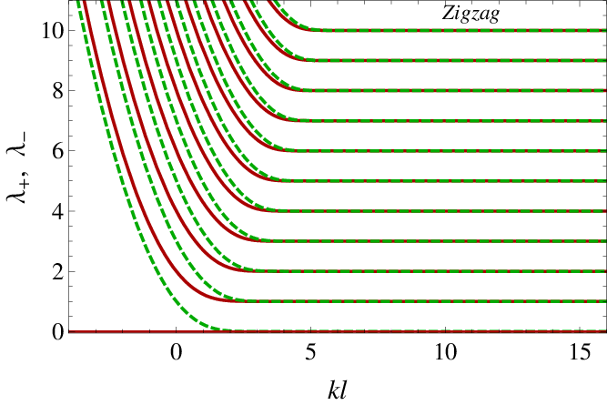
and $u_{+}(\xi)=v_{+}(\xi)=0$. By making use of the general properties of the parabolic cylinder function $D_{\nu}(z)$, we can understand some qualitative features of the energy spectrum even without solving the equations numerically. To this end, we need to know only that, for real $\nu$ and $z$, the function $D_{\nu}(z)$ has no real zeros when $\nu$ is negative, and has exactly $\left[\nu+1\right]$ real zeros when $\nu$ is nonnegative.[52] Here $\left[\nu+1\right]$ denotes the integer part of $\nu+1$. In view of this property, the necessary condition for Eq. (50) to be satisfied is $\lambda_{+}\geq 1$. By also including the possibility of the dispersionless mode, which is determined by $E=-\mu^{(+)}+\Delta^{(-)}$, we see that the complete spectrum in the $K_{+}$ valley (solutions of type I) has the following general structure:

where $n=1,2,\ldots$ is an index that labels different branches of solutions. By making use of the asymptotic behavior of the parabolic cylinder functions, one can show that $\lambda_{+}(kl,n)\simeq n$ when $kl\gg 1$. This is expected since large values of $kl$ correspond to the states in the bulk, whose wave functions are localized around $\xi\simeq 0$ or equivalently $y/l\simeq kl$. (In a system without edges, the index $n$ is identified with the usual Landau level index.)

Similarly, we can constrain the form of the spectrum in the $K_{-}$ valley (solutions of type II). The necessary condition for having a real solution to Eq. (52) is $\lambda_{-}\geq 0$. Thus, the energy spectrum in the $K_{-}$ valley has the following general structure:

where $n=0,1,2,\ldots$. Again, one can show that $\lambda_{-}(kl,n)\simeq n$ when $kl\gg 1$.

Our numerical results for $\lambda_{\pm}$ as functions of $kl$ are presented in Fig. 3. The solid and dashed lines represent $\lambda_{+}$ and $\lambda_{-}$, respectively. As expected, there exists an infinite tower of solutions that correspond to an infinite tower of Landau levels on a half-plane. In Fig. 3, we show only the first 11 solutions. We also added the constant solution $\lambda_{+}=0$ that, strictly speaking, represents only the dispersionless mode with the energy $E=-\mu^{(+)}+\Delta^{(-)}$ [see the first expression in Eq. (54)]. (Formally, $\lambda_{+}=0$ may also mean that $E=-\mu^{(+)}-\Delta^{(-)}$, but this is not an energy eigenvalue.)

By analyzing the structure of the spectrum together with the actual dependence of $\lambda_{\pm}$ on the wave vector, we can now determine when gapless modes exist in the spectrum of graphene on a half-plane with a zigzag edge. From Eqs. (54) and (55), we see that the necessary condition to have a zero energy state is that at least one of the following inequalities is satisfied:

From the fact that there exist branches with $\lambda_{+}\simeq 1$ and $\lambda_{-}\simeq 0$ at $kl\gg 1$, we see that this is also the sufficient condition.

An important point to emphasize here is that nonzero masses do not prevent the existence of the gapless edge states when the absolute value of $\Delta^{(+)}$ is less than the absolute value of $\mu^{(-)}$ at least for one choice of the spin. This is very similar to the conditions on a graphene ribbon of finite width,[39] except that there are no edge states associated with the second edge in the present work. Our results generalize the findings of previous studies on a half-plane,[17, 23] where only the case with a single nonzero order parameter (either mass or spin gap) was considered.

Two specific examples of energy spectra, with and without gapless modes, are given in Fig. 4. In the left panel, the first few Landau levels in the case of a small spin gap, which is modeled by $\mu_{\pm}=\mp 0.02\epsilon_{0}$ with the subscript index denoting the spin, and a larger singlet mass, which is given by $\Delta_{\pm}=\pm 0.08\epsilon_{0}$, are shown. Since $|\mu^{(-)}|<|\Delta^{(+)}|$, there are no gapless modes in this case. In the right panel of Fig. 4, the low-energy spectrum is shown for another choice of parameters, i.e., $\mu_{\pm}=\mp 0.08\epsilon_{0}$ and $\Delta_{\pm}=\pm 0.02\epsilon_{0}$, which satisfies the condition in Eq. (57). As expected, in this case there are gapless edge states in the spectrum. By taking into account the fact that the group velocities of gapless modes, $v_{x}=\partial E/\partial k|_{E=0}$, have opposite signs along the $x$-direction, the up- and down-spin states carry counter-propagating currents.[17, 23] It is also curious to note that these gapless states are chiral since they belong to a single valley ($K_{-}$).

Before concluding this section, it might be appropriate to mention that the examples of spectra shown in Fig. 4 may have a direct application to the case of graphene in a strong magnetic field. The corresponding choice of parameters with singlet, rather than triplet masses was taken in the same form as in the ground state around the neutral Dirac point, which was proposed in the dynamical model of Ref. 37. In fact, the spectra would look nearly the same also in the case of triplet masses, except perhaps for an overall shift of the dispersionless modes, which depend not only on the absolute value but also on the sign of the mass terms.

In this section, we analyze the spectrum of edge modes in the case of an armchair edge. We take the armchair edge parallel to the $y$-direction, as shown in Fig. 2. In this case, it is convenient to use a different Landau gauge with $(A_{x},A_{y})=(0,Bx)$. Accordingly, the solutions of Eq. (37) are translation invariant along the $y$-direction,

Then, the corresponding differential equations for functions $u_{\pm}(x,k)$, which are rewritten in terms of the dimensionless variable $\xi=x/l+kl$, coincide with Eq. (39). The expressions for the eliminated components $v_{\pm}(\xi)$, however, slightly differ from Eq. (40), and are given by

We consider a graphene sheet in the half-plane $x>0$. Since the armchair edge has lattice sites of both $A$ and $B$ types, the wave function should vanish at both these sites along the $x=0$ line,[46, 48, 23]

Note that armchair boundary conditions mix the chiralities associated with the $K_{+}$ and $K_{-}$ valleys. The general solutions for the $u_{\pm}(\xi)$ functions have the same form as in Eqs. (43) and (44),

but with $\xi=x/l+kl$. By using the relations in Eqs. (59) and (45), we also obtain the explicit expression for $v_{\pm}(\xi)$ functions,