UHE tau neutrino flux regeneration while skimming the Earth
Abstract
The detection of Earth-skimming tau neutrinos has turned into a very promising strategy for the observation of ultrahigh-energy cosmic neutrinos. The sensitivity of this channel crucially depends on the parameters of the propagation of the tau neutrinos through the terrestrial crust, which governs the flux of emerging tau leptons that can be detected. One of the characteristics of this propagation is the possibility of regeneration through multiple conversions, which are often neglected in the standard picture. In this paper, we solve the transport equations governing the propagation and compare the flux of emerging tau leptons obtained allowing regeneration or not. We discuss the validity of the approximation of neglecting the regeneration using different scenarios for the neutrino-nucleon cross sections and the tau energy losses.
pacs
95.55.Vj, 13.60.-r, 14.60.FgI Introduction
With the advent of a new generation of large-scale detectors of cosmic radiation, the observation of high-energy cosmic neutrinos produced in distant astrophysical sites or possibly by other, more exotic, mechanisms has become one of the major challenges of astroparticle physics. In both astrophysical and exotic models, substantial fluxes of electron and muon neutrinos are expected from the disintegration of charged pions (and kaons) produced in the interaction of accelerated particles with ambient matter and radiation, either at the source location or between the source and the observer. Given the large distances traveled by these cosmic neutrinos, approximately equal fluxes in and are expected on Earth as a result of flavor mixing and oscillations [1, 2]. Important efforts are ongoing to build dedicated neutrino telescopes both in the Southern [3, 4] and Northern [5, 6, 7, 8] hemisphere, opening a window on the neutrino sky in the energy range . At even higher energies, other promising experiments are developing the detection of coherent radio emission produced by neutrino-induced showers in matter [9, 10, 11, 12, 13, 14, 15].
Interestingly, recent studies have shown that the new generation of ultrahigh-energy (UHE) cosmic ray detectors such as the Pierre Auger Observatory [16] and the HiRes Fly’s Eye detector [17] have a comparable detection potential for UHE neutrinos in the range of energies , where neutrinos are expected to be produced in the interaction of UHE cosmic rays with the cosmic microwave background [18]. It is long known that downward-going showers induced by neutrinos that penetrate deep in the atmosphere can in principle be identified at large zenith angles () where no background is expected from hadronic primaries [19, 20]. It was also pointed out more recently that the presence of in the cosmic neutrino flux provides another promising channel of detection for air shower detectors [21, 22]. Upward-going UHE tau neutrinos that graze the Earth just below the horizon (often referred to as “Earth-skimming neutrinos”) are indeed likely to interact in the crust and produce a tau lepton which may emerge and initiate an observable air shower, provided it does not decay too far from the detector.
The sensitivity to such UHE Earth-skimming neutrinos crucially depends on the conditions of the propagation through the terrestrial crust, and on the correct estimation of the flux of leptons that emerge from the Earth. This propagation problem has been widely discussed in different contexts and with different approximations [23, 24, 25, 26, 27, 28, 29]. An exhaustive treatment should account for and neutral-current (NC) and charged-current (CC) interactions with nucleons, decay and energy losses. However the full coupled transport equations admit no analytical solution, and even in the case of Monte Carlo calculations, simplifications are usually made such as dropping the weak interactions and neglecting multiple regenerations of the .
Such approximations are defendable in the standard case where the characteristic lengths for the CC interaction ( km, at 1 EeV) and for the decay ( km) are larger than that for energy losses ( km). However, they might be challenged in other, more exotic scenarios. The knowledge of the neutrino cross section and the tau energy losses in the EeV energy range is indeed limited [30, 31], and these could be significantly affected at center-of-mass energies beyond the TeV by the onset of new physics beyond the standard model. Several studies have even suggested that the comparison of the flux rates between down-going and Earth-skimming neutrinos could actually help constraining the neutrino properties at ultrahigh energies, where no direct measurements exist [32, 33].
All these considerations pinpoint the necessity of an accurate determination of the flux of emerging leptons. In this context, it is important to correctly describe all the contributions to the flux and to assess the impact of simplifications in the description of the propagation problem.
The present paper therefore focuses on understanding the effects of the and regeneration while skimming the Earth on the flux of emerging leptons in different scenarios for the neutrino-nucleon cross section and for the energy losses. In Sec. II, we present the transport equations for the and propagation, and the scenarios to be studied. In Sec. III, we compare the flux of emerging taus for different conditions of propagation. Finally, we present our conclusions in Sec. IV.
II propagation through the Earth: the general picture
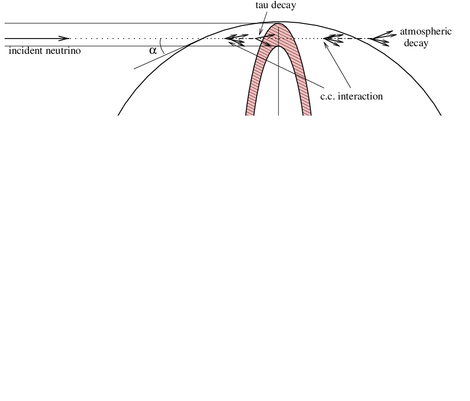
The geometry of the propagation problem is described in Fig.1, where an example of regeneration chain through multiple CC interactions and decays is sketched. Given a beam of parallel neutrinos incident on the Earth at a given angle , the problem becomes unidimensional and the flux of leptons that emerge only depends on the path length traveled across the rock. In the hypothesis of a spherical Earth with a crust of constant density, this length is directly related to , which is also the angle of the emerging tau.
II.1 Transport equations
We reproduce here a classical formulation in terms of the transport equations that describe the evolution of the and fluxes, and , along their path through the Earth, accounting for all possible production and absorption processes taking place within an infinitesimal :
| (1) |
Here and are the mean free paths corresponding respectively to NC and CC interactions of the incident , while corresponds to the CC interaction, which regenerates a . is the tau lepton lifetime.
The transport equation for the can be inferred in a similar way. In this case, the small inelasticity of the radiative interactions allows us to use the continuous energy loss approximation [34]. Defining , the equation reads:
| (2) |
where and are now the mean free paths associated with the NC and CC interactions, and is the decay length corresponding to .
We are thus left with a system of two coupled, integro-differential equations, which cannot be solved analytically without making simplifying assumptions on the nature and the respective importance of the interactions that both the and the can undergo. To preserve the generality of the solution we use a Monte Carlo simulation that includes all the processes listed above and follows the incident particle all the way through the rock, deciding at each step on its fate according to the distributions encoded in Eq.1 and Eq.2.
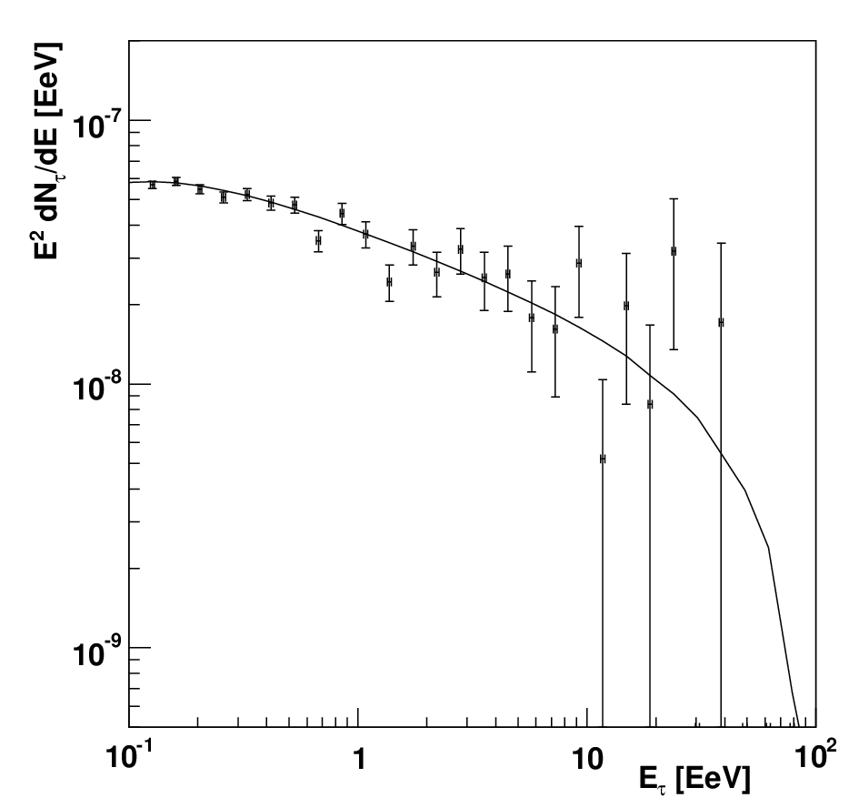
An iterative method that also allows us to avoid simplifications was proposed in [35], and further discussed in [27] and in [36]. Our equations differ from those in [27, 36] in that we also include the two terms describing NC interactions in the transport equation for . Taking into account this generalization, we have applied the iterative method (see the Appendix for details) to crosscheck the results from the Monte Carlo simulation. In Fig. 2, we show the good agreement between both calculations for the flux of emerging leptons given an incident tau neutrino flux = 4.6107 E EeV-1 sr-1.
II.2 Cross Sections
In the framework of the standard model, the neutrino-nucleon () CC and NC cross-sections, and , describe deep-inelastic scattering processes. They are expressed in terms of the structure functions of the nucleon, which in turn depend on the individual parton distribution functions (PDFs). The PDFs are obtained from measurements at accelerators, in determinate ranges of Bjorken- and momentum transfer . However, the range of parameters probed by the UHE neutrinos, and up to , is outside the measured domain and therefore extrapolations are needed.
We choose as a benchmark for the standard cross section a recent parametrization presented in [30], which fits to updated HERA data:
| (3) | |||||
As pointed out in the same paper, another, more speculative approach based on the color glass condensate formalism [37] has also been put forward recently to account for saturation at very low . We will also consider this case and use the following approximate parametrization deduced from Fig. 1 of [30]:
| (4) | |||||
as an example of low cross section.
On the other hand, plenty of models using new physics predict an enhancement of the neutrino cross section [38]. As an example of high cross section, we will use
| (5) |
without assuming any particular model.
II.3 Tau energy losses
The energy losses are usually parametrized using the following formula:
| (6) |
where is practically constant and accounts for ionization processes, while includes the radiative contributions from bremsstrahlung (b), pair production (pp) and photonuclear (pn) interactions of the .
For the purpose of our analysis, we adopt the same strategy as in the previous section and extract from existing computations [31, 39] a panel of ad-hoc parametrizations of in the relevant range of energy, representative of the values found in the literature. The set of parametrizations under study is the following (valid in the range EeV EeV):
respectively for a standard, a high and a low value of the energy loss parameter .
III The flux of emerging taus: results and comparisons


The Earth-skimming technique has been recently used to search for with the HiRes telescopes [17] and the Pierre Auger Observatory [16]. While both detectors have a similar energy threshold ( 0.1 EeV), they are sensitive to a different range in the emerging angle of the leptons. The latter detects the particles from the air shower initiated by the decay that reach the ground and, hence, the detector will only be triggered by leptons slightly up-going (). The former is designed to record the faint ultraviolet light emitted by nitrogen molecules that are excited as the shower traverses the atmosphere; it is therefore sensitive to leptons emerging with larger angles.
In figure 3, we present the results obtained with the Monte Carlo approach for the flux of emerging leptons with an angle up to 3∘ and 15∘ produced by an incident tau neutrino flux = 4.6 10 EeV-1 sr-1. All cross sections and energy loss parameters are here set to standard values, as defined in Secs. II.2 and II.3. The effect of the regeneration is negligible if only almost horizontal emerging leptons () are taken into account. On the other hand, if the detector is sensitive to larger angles and energies down to a fraction of EeV, neglecting the regeneration becomes important already within this standard picture (30 less leptons at 0.3 EeV for an incident neutrino flux ).


The approximation of neglecting the regeneration seems thus to be safe in the standard picture for detectors only sensitive to almost horizontal showers. However, we will now show that this approximation is questionable even for them as soon as one considers non-standard scenarios. We have investigated the effect of the regeneration for those detectors using the set of parametrizations defined in Secs. II.2 and II.3. These expressions do not constitute an exhaustive list of all the alternative and exotic models that exist in the literature, but rather a selection of a few examples that allow us to point out the relevance of this process. The combinations of cross sections and tau energy losses should be chosen on basis of coherent PDFs but this coherency is hard to assert even inside the frame of the standard model. Therefore, we chose to investigate the regeneration effects for the 33 possible combinations, which is sufficient to provide a qualitative answer to the question raised in this paper.
As a starting point, one should however notice that the regeneration requires the to be converted back into a before losing too much energy, and then this to undergo another CC weak interaction to produce a again. Hence, one expects that a higher energy loss or a lower cross section will reduce the effect of the regeneration, while, on the other hand, a higher cross section or a lower energy loss will enhance it. This is indeed what we find. In the following, we focus on the particular combinations for which the regeneration is not negligible anymore, and compare them to the standard case, essentially on the basis of monoenergetic incident beams of ’s. This is because the power-law spectrum usually assumed for cosmic neutrinos, although adequate to look at the global flux of emerging leptons, is completely dominated by the lowest energies, while the behavior at the highest energies may be important for harder fluxes of incident neutrinos.
In Fig. 4-7, we show the flux of leptons produced by incident neutrinos at given energies (0.3, 3 and 30 EeV) and with an angle up to 3∘, for the following combinations of parametrizations: (the same as used in Fig. 3), , and . For a standard choice of parametrizations, one can see from Fig. 4 that the impact of regeneration is completely negligible at low neutrino energies. As the energy increases, however, the lowest-energy part of the spectrum starts to be significantly underestimated (15 less taus for 30 EeV incident neutrinos). This effect is washed out in the case of an incident neutrino flux , for which the contribution of the highest-energy part of the neutrino spectrum is negligible; but it could affect the spectrum of emerging ’s if the neutrino flux were harder. For the other cases, the lowest-energy range of the spectrum becomes underestimated already for incident with energy of 0.3 EeV. For the combination , one loses about 70 of the leptons emerging from the Earth if the regeneration is neglected, even if assuming an incident flux of neutrinos (Fig. 8).

The neutrino flux can be regenerated through the decay and the CC weak interaction. We present our results in a form that allows us to disentangle the two effects: the dotted histograms in Fig. 4,5,6,7 account for regeneration through the weak interaction of the only, while the solid ones include both effects. As can be appreciated in the figures, the CC contribution is negligible at all energies in most scenarios. It only becomes important for ’s at the highest energies ( EeV), in the energy range between 0.3 and 3.0 EeV of the emerging spectrum, if a high cross section is assumed (Figs. 5 and 7). There, the effect is at the level of that from the regeneration through the decay.
IV Conclusion
In this paper, we have studied the mechanism of regeneration of the flux while crossing the Earth, to investigate its effect on the flux of emerging leptons. Assuming a detector with an energy threshold of 0.1 EeV and sensitive only to taus with an emerging angle below 3∘, the effect is negligible for a flux of incident neutrinos with the standard values of cross sections and energy losses. But we have shown that this is not valid for other assumptions on the detector performance, neither for less standard values of the weak cross section or tau energy losses. On the one hand, neglecting the regeneration leads to about 30 underestimation on the integrated flux for a detector sensitive up to 15∘. On the other hand, the underestimation of the ’s emerging from the Earth with an energy greater than 0.1 EeV and an emerging angle below 3∘ may reach 70 for the different values of and studied in this paper. Moreover, the error made in the computation of the flux of emerging taus can be even larger for a harder flux of incident neutrinos since the contribution of the regeneration effect increases with the energy of the incident neutrino.
The simplification of neglecting the regeneration is thus only safe for particular values of the physical properties playing a role on the propagation and specific detectors. It may lead to a significant underestimation of the flux of emerging ’s when looking at nonstandard values of the weak cross section or tau energy losses. Therefore, it should be carefully treated and accounted for when studying the systematics due to the uncertainties on those properties or while using the Earth-skimming technique to test for instance higher weak cross-sections. Similarly, one should carefully check the effect for the characteristics of the actual detector before neglecting the regeneration.
Acknowledgments
The authors would like to thank their colleagues of the Pierre Auger Collaboration for useful discussions and suggestions. O. B. B. is supported by the Ministerio de Educación y Ciencia of Spain through the postdoctoral grant program. V.V.E. acknowledges support from the European Community Framework Program through the Marie Curie Fellowship MEIF-CT-2005 025057.
Appendix A Iterative solution of the transport equations
We reproduce here a numerical method proposed in [35, 27], generalizing it to take into account the NC weak interaction of the lepton. We start from a solution of order 0 and iterate it up to get a solution that satisfies the relation as given by Eq. 1 or 2. For numerical reasons, it is better to work with numbers between 0 and 1 so that we write the equations in terms of the deviation to the solution of order 0, , rather than in terms of itself. We therefore assume that the solution is of the form
where accounts for the possible sources of depletion of at an energy , and is a function to be determined, which includes all contributions to the regeneration of at the same energy.
can be obtained iteratively by forcing it to satisfy the transport equations, viewed as a recurrence relation with the initial condition :
| (7) |
As the two equations are coupled, it is necessary to know at a given order to proceed with the iteration at the next order. Following the same philosophy as above, we assume that the solution of Eq.2 for is of the form:
where the following notations have been introduced:
and . The equation for then reads:
again with ). Practically, the iteration can be stopped as soon as n=3.
References
- [1] S. Fukuda et al. [Super-Kamiokande Collaboration], Phys. Rev. Lett. 86 (2001) 5656 [arXiv:hep-ex/0103033].
- [2] J. G. Learned and S. Pakvasa, Astropart. Phys. 3 (1995) 267 [arXiv:hep-ph/9405296].
- [3] E. Andres et al., Astropart. Phys. 13 (2000) 1 [arXiv:astro-ph/9906203].
- [4] A. Karle [IceCube Collaboration], Nucl. Instrum. Meth. A 567 (2006) 438 [arXiv:astro-ph/0608139].
- [5] J. Carr [ANTARES Collaboration], Nucl. Instrum. Meth. A 567 (2006) 428.
- [6] I. Amore [NEMO Collaboration], Int. J. Mod. Phys. A 22 (2007) 3509 [arXiv:0709.3991 [astro-ph].
- [7] G. Aggouras et al., Nucl. Instrum. Meth. A 552 (2005) 420.
- [8] V. Aynutdinov et al. [Baikal Collaboration], Nucl. Instrum. Meth. A 567 (2006) 433 [arXiv:astro-ph/0507709].
- [9] S. W. Barwick et al. [ANITA Collaboration], Phys. Rev. Lett. 96 (2006) 171101 [arXiv:astro-ph/0512265].
- [10] I. Kravchenko et al., Phys. Rev. D 73 (2006) 082002 [arXiv:astro-ph/0601148].
- [11] N. G. Lehtinen et al. Phys. Rev. D 69 (2004) 013008 [arXiv:astro-ph/0309656].
- [12] P. W. Gorham et al., Phys. Rev. Lett. 93 (2004) 041101 [arXiv:astro-ph/0310232].
- [13] T. H. Hankins et al., MN-RAS 283 (1996) 1027
- [14] C. W. James and R. J. Protheroe, arXiv:0802.3562 [astro-ph].
- [15] G. Swarup and S. Panda, arXiv:0805.4304 [astro-ph].
- [16] J. Abraham et al. [Pierre Auger Collaboration], Phys. Rev. Lett. 100 (2008) 211101 [arXiv:0712.1909]
- [17] K. Martens [HiRes Collaboration], arXiv:0707.4417 [astro-ph].
- [18] F. W. Stecker et al., Phys. Rev. Lett. 66 (1991) 2697 [Erratum-ibid. 69 (1992) 2738].
- [19] V. S. Berezinsky and A. Yu. Smirnov, Astrophys. Space Science 32 (1975), 461;
- [20] K. S. Capelle et al., Astropart. Phys. 8 (1998) 321 [arXiv:astro-ph/9801313].
- [21] A. Letessier-Selvon, AIP Conf.Proc. 566 (2000) 157-171, arXiv:0009444 [astro-ph].
- [22] D. Fargion, Astrophys. J. 570 (2002) 909 [arXiv:hep-ph/0002453] and references therein.
- [23]
S. I. Dutta, M. H. Reno, I. Sarcevic and D. Seckel,
Phys. Rev. D 63 (2001) 094020 [arXiv:hep-ph/0012350]. - [24] X. Bertou et al., Astropart. Phys. 17 (2002) 183 [arXiv:astro-ph/0104452].
- [25] J. L. Feng et al., Phys. Rev. Lett. 88 (2002) 161102 [arXiv:hep-ph/0105067].
- [26] S. Bottai and S. Giurgola, Astropart. Phys. 18 (2003) 539 [arXiv:astro-ph/0205325].
- [27] J. J. Tseng, T. W. Yeh, H. Athar, M. A. Huang, F. F. Lee and G. L. Lin, Phys. Rev. D 68 (2003) 063003 [arXiv:astro-ph/0305507].
- [28] E. Bugaev, T. Montaruli, Y. Shlepin and I. Sokalski, Astropart. Phys. 21 (2004) 491 [arXiv:hep-ph/0312295].
- [29] C. Aramo et al., Astropart. Phys. 23 (2005) 65 [arXiv:astro-ph/0407638].
- [30] L. A. Anchordoqui, A. M. Cooper-Sarkar, D. Hooper and S. Sarkar, Phys. Rev. D 74 (2006) 043008 [arXiv:hep-ph/0605086].
- [31] N. Armesto, C. Merino, G. Parente and E. Zas, Phys. Rev. D 77 (2008) 013001 [arXiv:0709.4461 [hep-ph]].
- [32] S. Palomares-Ruiz, A. Irimia and T. J. Weiler, Phys. Rev. D 73 (2006) 083003 [arXiv:astro-ph/0512231].
- [33] L. Anchordoqui, T. Han, D. Hooper and S. Sarkar, Astropart. Phys. 25 (2006) 14 [arXiv:hep-ph/0508312].
- [34] O. Blanch et al., Phys. Rev. D 77 (2008) 103004 [arXiv:hep-ph/0802.1119].
- [35] V. A. Naumov and L. Perrone, Astropart. Phys. 10 (1999) 239 [arXiv:hep-ph/9804301].
- [36] E. Reya and J. Rodiger, Phys. Rev. D 72 (2005) 053004 [arXiv:hep-ph/0505218].
- [37] L. D. McLerran and R. Venugopalan, Phys. Rev. D 50 (1994) 2225 [arXiv:hep-ph/9402335]; see also E. Iancu and R. Venugopalan, in Quark and Gluon Plasma (World Scientific, Singapore, 2004) Vol. 3, p. 249.
- [38] see T. Han and D. Hooper, New J. Phys. 6 (2004) 150 [arXiv:hep-ph/0408348] and references therein.
- [39] S. I. Dutta, Y. Huang and M. H. Reno, Phys. Rev. D 72 (2005) 013005 [arXiv:hep-ph/0504208].