An efficient approach of controlling traffic congestion in scale-free networks

Operations in the internet such as browsing webpages in the World Wide Web (WWW), sending e-mails, transferring files via ftp, searching for information, and electronic shopping, etc. have become part of daily life for many people. These activities have opened up exciting opportunities for sharing information, economic transformation, and other activities on a global scale [1, 2]. The internet, however, is not perfect. For example, intermittent congestion in the internet, similar to traffic congestion in highway systems, has been observed [3]. Similar phenomena can be also of relevance in other communication networks, such as the transportation network in airlines and the postal service network. A key problem in communication networks is, therefore, to understand how one can control congestion and maintain a normal and efficient functioning of the networks.

Several models of communications in a computer network have been extensively studied [4, 5, 6, 7, 8, 9, 10, 11, 12, 13, 14, 15, 16]. In these models, the information processors are routers. Their function is to route the data packets to their destinations. In a computer network, a node may be a host or a router. A host can create messages or data packets for targeted destinations and receive packets from other hosts. A router finds the shortest path between the origin of the message and the destination of each packet and forwards the packet one step closer to the destination along the shortest path in each time step. The shortest path is the path with the smallest number of links. Previous studies have mostly been focused on three different computer network models: (i) the nodes at the edge of the network are hosts and the inner nodes are routers [9], (ii) all the nodes are both hosts and routers [10, 13, 14], and (iii) some of the nodes are hosts and the rest are routers [11, 15, 16]. However, these models were studied with the underlying networks being a two-dimensional lattice [9, 10, 11, 15] and a Cayley tree [12, 13, 14]. As the internet shows a heterogeneous structure with a scale-free degree distribution [17, 18], a more realistic network model for communications should be heterogeneous. Besides the internet and its related networks such as WWW [19, 20, 21] and email networks [22], many other networks also show the scale-free behavior. These networks include, for example, the telephone network [23], the biological network in proteins [24], and the networks of sexual contacts [25, 26]. Some networks, such as the collaboration network among scientists [27], show a mixed feature of scale-free and exponential distributions. In fact, the study of the science of complex networks has become an important interdisciplinary area of research. The problem of efficiency in delivering messages or data packets in communication networks has been addressed recently by Arenas et al. [28, 29, 30], Moreno et al. [31, 32, 33], and Zhao et al. [34]. Arenas et al. focused on finding the optimal network topologies for searches in complex networks, while Moreno et al. studied the dependence of the jamming transitions on routing strategies. A common feature in previous studies is that the creation and delivering rates of packages do not change from node to node. As the nodes in a complex network could have very different properties, e.g., degrees, a more realistic assumption is that the package creation rate and delivering rate at a node become degree-dependent. In the internet, an important site has more users and hence a larger message or package creation and delivering rates. A recent study by Zhao et al. [34] considered the case of non-uniform package delivering rates, but the creation rate was taken to be a constant.

In the present work, we study traffic in networks with non-uniform package creation and delivering rates. An important quantity in communication networks is the critical package creation rate that signifies a transition from a non-congested or free flow regime to a congested regime. Below the critical rate, a non-congested steady state is reached after the transient in which the data packets created can be efficiently handled by the nodes. Above the critical rate, a congested phase is reached where the number of packets accumulated in the system increases with time. The value of critical rate thus measures the capacity of efficient communication inside the network. Here, we study the critical rate in networks where the package creation and delivering rates are node-dependent. In particular, we present an efficient approach to enhance the capacity of communications in scale-free networks.

The paper is organized as follows. Section II defines the model with node-dependent package creation and delivering rates. In Section III, we present results of numerical simulations and study the interplay between the critical and delivering rates in determining non-congested or congested traffic in a network. Section IV explains the observed features in the numerical results analytically. We summarize the paper in Sec. V.

The nodes in a complex network such as the internet may represent very different entities. For example, some nodes may just be individuals and other may represent big companies or universities. Obviously, different nodes will have different rates of creating messages. The nodes, depending on their connectivity to other nodes and perhaps hardware, also have different rates of delivering messages. Here, we present a more realistic model of communication in complex networks that includes node-dependent creation and delivering rates. Our model is a modification on several previous models [28, 29, 30, 31, 32, 33, 34]. We assume that for a node $i$ with degree $k_{i}$, the message creation rate $\lambda k_{i}$ is proportional to its degree, with $\lambda$ being a constant. For message delivering, each node should handle at least one packet or message in each time step. Therefore, we assume a delivering rate of $1+\beta k_{i}$ for a node with degree $k_{i}$, with $\beta\geq 0$ being a parameter of the model. Our model thus represents the realistic situation that a busy node with larger $k_{i}$ has higher rates of generating and delivering messages.

For the underlying network, we use a model in which the exponent of the degree distribution can be tuned. A scale-free network with $P(k)\sim k^{-\gamma}$ can be constructed by incorporating preferential attachments in a network-growing process [36, 35]. The Barabasi and Albert model [36] assumes the probability $\Pi_{i}$ for a node $i$ to attract a link from a newly added node to be $\Pi_{i}\sim k_{i}$. The model gives an exponent $\gamma=3$ [36] for the degree distribution. On the other hand, a random growing network can be constructed by assuming a node-independent $\Pi_{i}$. Many networks show characters that are somewhat intermediate of scale-free and random. For them, the degree distribution shows a mixed feature of the two characters [27]. This implies that the probability $\Pi_{i}$ of attracting a new link should contain both preferential and random features. One of the present authors proposed a hybrid model [37] in which $\Pi_{i}\sim(1-p)k_{i}+p$, where $0\leq p\leq 1$ is a parameter representing the probability that a newly added node establishes its new links by random attachments and $(1-p)$ is the probability that new links are established by preferential attachments. The degree distribution was shown to be [37] $P(k)\sim[k+p/(1-p)]^{-\gamma(p)}$ with an exponent $\gamma(p)=3+p/[m(1-p)]$, where $m$ is the number of new links per node. The $p=0$ limit reduces to the $P(k)\sim k^{-3}$ behavior and the $p\rightarrow 1$ limit gives the random growing network behavior of $P(k)\sim e^{-k/m}$. Here, we use this model as our underlying network for studying communications in networks.

Once the network of a certain value of $p$ is constructed, the dynamics of creating and delivering messages is implemented as follows. Each node plays the dual role of a host and a router, with its creation and delivering rates assigned according to its degree. Details of the dynamics are listed as follows.

The parameters $\lambda$ and $\beta$ thus control the number of messages or packages in the system. A small (high) value of $\lambda$ corresponds to fewer (more) packets. For simplicity, each packet is labeled by two pieces of information: the time of creation and its destination. Qualitatively, the total number of packets created at each time step is $\sum_{i=1}^{N}\lambda k_{i}\approx\sum_{i=1}^{N}\lambda\langle k\rangle=2m\lambda N$ for a growing network of $m$ newly added links per node and a total of $N$ nodes. At the same time, the maximum number of packets processed by the nodes is $\sum_{i=1}^{N}(1+\beta k_{i})\approx(1+2m\beta)N$. When the number of new packets added to the system equals the number of packages removed upon arrival at each time step, the network runs in the range of Little law [38] and there is no congestion. For scale-free networks, the structure is heterogeneous in the sense that some nodes have many more links. As messages are sent via the shortest paths, they are likely to pass through the nodes with more links. If every node has the same delivering rate, these nodes will have more accumulated messages and a high chance of jamming. In contrast, random networks do not have hubs with high degrees and thus the structure is relatively “homogeneous”. Therefore, congestion is easier to occur in scale-free networks than random networks. As most of the real-life networks are scale-free, the control of congestion in these networks is of critical importance. For example, an intuitive but not so efficient approach is to increase the value of $\beta$ for the nodes. We will refer to this approach of having identical values of $\beta$ for all nodes as the normal approach.

The number of nodes in a communication network is typically very large and there is no central organizer to manage the development of the whole network. It is, therefore, very difficult to have a realistic mechanism to increase $\beta$ for all nodes at the same time. Realistically, larger companies and academic institutions could increase their local value of $\beta$ more readily. Noting that congestion is more likely to occur at the nodes with many links in scale-free networks, one may significantly reduce congestion by selectively increasing the delivering rates of the nodes with high degrees. Therefore, we suggest that a possible cost-effective way to control congestion is to ask the nodes with larger links to increase their value of $\beta$. Here, we study a model in which a fraction $f$ of nodes with high degrees are assigned a finite value of $\beta>0$, and the rest are assigned $\beta=0$. This models the higher message-processing capability of the hubs in a network. We refer to this model as the efficient approach. In this model, the maximum number of packets processed in a time step is $(N+\sum_{i\in f}\beta k_{i})$, where the sum is over the nodes with finite $\beta$. Results of numerical simulations show that the efficient approach performs comparably with the normal approach. In the following sections, we compare results of the two approaches and explain the results analytically.

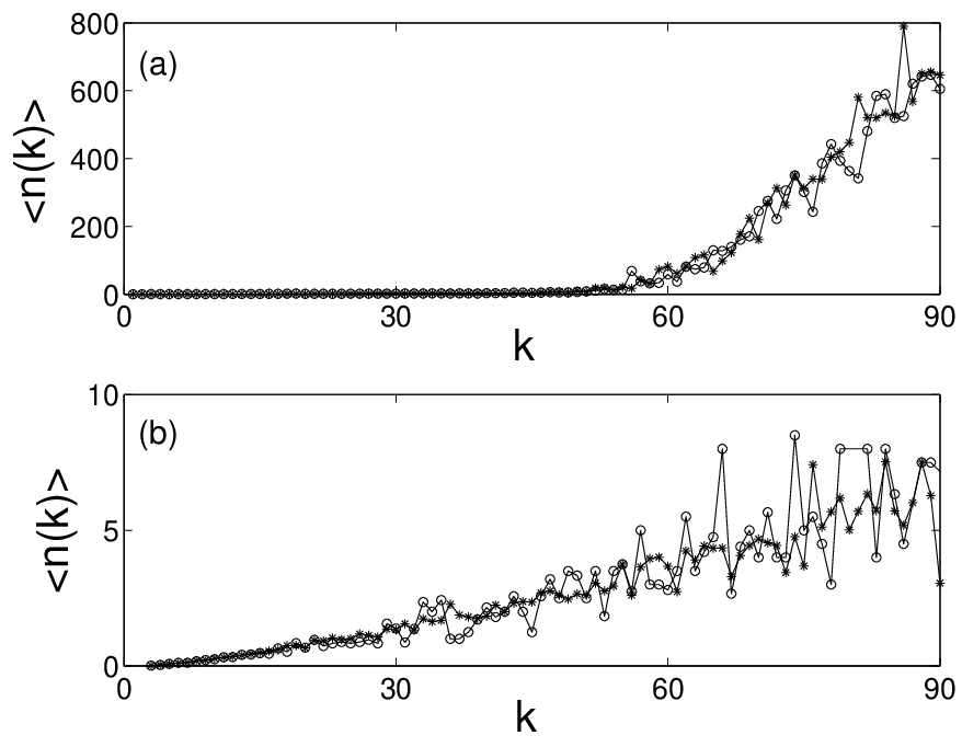
The network is constructed as described in Sec. II and in Ref.[37], with $N=1000$, $m=3$ and different values of $p$. The dynamics of package delivering is then implemented on the network. We first consider the normal approach in which all the nodes have the same value of $\beta$. Intuitively, a larger $\beta$ can assure free traffic flow for a larger creation rate signified by a larger value of $\lambda$. Here, we fix $\lambda=0.01$ and take $\beta=0,0.05$, and $0.1$ to illustrate the effects. For $\beta=0$, every node has a creation rate $\lambda k_{i}$ depending on $k_{i}$, but the delivering rate of forwarding at most one message per time step applies to all nodes. To understand how congestion occurs, we calculate the average number of packets $\langle n(k)\rangle$ on the nodes with a given number of links $k$. This quantity serves to show where are the longest queues. Numerical simulations show that they are the nodes with more links, as shown in Fig.1 (circles) for systems after $t=500$ time steps. The results are obtained by averaging over $100$ different realizations for a given set of parameters. Fig.1(a) shows the results for random growing networks ($p=1$) and Fig.1(b) shows the results for scale-free network ($p=0$). It is clear that in both cases, the nodes with large number of links are more likely to be congested. Comparing the results in Fig.1(a) with (b), one sees that the accumulation of packets in scale-free networks is much pronounced than that in random networks. The results indicate that congestion is much easier to occur in scale-free networks. For $\beta=0.05$ (squares in Fig.1), the accumulation of packets is greatly suppressed in both limits of the underlying network. In particular, congestion almost disappeared in the case of random growing networks. For even higher message-processing capability $\beta=0.1$ (stars in Fig.1), congestion disappeared in both the random and scale-free networks. These results also indicate that there exists a critical value $\beta_{c}$ for a given $\lambda$ so that congestion occurs for $\beta<\beta_{c}$. We will study the dependence of $\beta_{c}$ on $\lambda$ in networks of different underlying structures characterized by $p$.

Another point that is worth noticing is that the nodes in a range of small to intermediate degrees (see inset in Fig.1) in the normal approach usually carry fewer messages than the uniform delivering capacity. The result implies that it is unnecessary for these nodes to have a higher delivering capability characterized by a finite $\beta$. It leads us to consider the efficient approach. In the scale-free ($p=0$) limit as shown in Fig.1(b), the degree distribution is a power law and the nodes that carry $k\geq 20$ account for only $3\%$ of all the $N=1000$ nodes. To illustrate the idea of the efficient approach, we take $f=3\%$, i.e., we assign a non-vanishing $\beta$ only to nodes that have $k\geq 20$. Figure 2 compares results of the normal approach (stars) and the efficient approach (circles) for two values of $\beta$. Obviously the difference in $\langle n(k)\rangle$ between the two approaches is small in scale-free networks. As the efficient approach does not require all nodes to be equipped with the same capability, it represents a more practical and cost-effective way to avoid jamming. In contrast, we note that the efficient approach does not work so well in random networks ($p=1$). It is because the degree distribution is narrower compared with the $p=0$ case. Therefore, the queues are more evenly distributed among the nodes and congestion is not restricted to the nodes among the highest degrees. It is thus necessary to assign a finite $f$ to a larger fraction of nodes to avoid congestion, and the two approaches become similar.

We define $\langle n_{1}(t)\rangle$ to be the average number of messages per node. In the congested regime, $\langle n_{1}(t)\rangle$ increases with time $t$. In the non-congested regime, $\langle n_{1}(t)\rangle$ fluctuates around a constant. The slope of $<n_{1}(t)>$ after the transient can thus be used to determine $\beta_{c}$ [30, 32]. For a given $\lambda$, the slope gradually decreases as $\beta$ increases. The value of $\beta$ that the slope becomes zero gives $\beta_{c}$. For $\beta>\beta_{c}$, the slope remains zero. Figure 3(a) shows typical results with $\lambda=0.01$ for three different values of $\beta$ within the efficient approach ($f=3\%$). For $\beta=0.05$, $\langle n_{1}(t)\rangle$ increases with time without bound. The critical value is found to be $\beta_{c}=0.059$ where the slope vanishes. For $\beta=0.7>\beta_{c}$, the slope remains zero. As congestion mainly occurs at the nodes with large degrees, the number of messages $\langle n_{2}(t)\rangle$ averaged over the $3\%$ of nodes should also show a similar behavior with time. It is indeed the case (see Fig.3(b)).

Next, we study the dependence of $\beta_{c}$ on the creation rate characterized by $\lambda$ in scale-free and random growing networks. Fig.4(a) shows the results in the scale-free limit ($p=0$) for both the normal (circles) and efficient (stars) approaches. For small $\lambda$, $\beta_{c}$ vanishes as the default delivering rate of one message per time step is already sufficient to handle the small message creation rate. For the range of $\lambda$ shown in the figure, $\beta_{c}$ increases linearly with $\lambda$ and the two approaches give similar results. This again shows that the efficient approach performs as good as adjusting $\beta$ across the whole network. It should be noted that for larger values of $\lambda$ (beyond the range shown here), assigning a finite $\beta$ to only the top $3\%$ of nodes may not be sufficient to avoid congestion. For random growing networks ($p=1$), we show $\beta_{c}(\lambda)$ in Fig.4(b) only for the normal approach, as the efficient approach becomes similar to the normal approach. Qualitatively, $\beta_{c}(\lambda)$ shows a similar behavior to that in scale-free networks. Quantitatively, $\beta_{c}=0$ for a larger range of $\lambda$ in random networks and the slope of the linear dependence in $\beta_{c}(\lambda)$ is smaller. It is because the nodes in random networks are more “homogeneous” and a queue will not emerge at the hubs for small $\lambda$ as in the case of scale-free networks. The function $\beta_{c}(\lambda)$ in Fig.4(a) also divides the $\beta$-$\lambda$ space into two regions. The region above the line represents a non-congested or free flow regime and that below the line represents a congested regime. Thus for given $\lambda$, one can go from a congested to a non-congested regime by increasing $\beta$. Similarly, for a given $\beta$, one can go from a non-congested regime to a congested regime by increasing $\lambda$. Although we only present results for networks with $N=1000$ nodes, we have checked that the linear dependence of $\beta_{c}$ on $\lambda$ also holds for networks with larger $N$.

In this section, we aim at explaining the behavior of $\beta_{c}(\lambda)$ quantitatively. As discussed, $\langle n_{1}(t)\rangle$ behaves differently for $\beta<\beta_{c}$ and $\beta\geq\beta_{c}$. In the non-congested or free flow regime, the steady state satisfies the Little’s law [38], which states that the number of delivered messages is balanced by the number of newly created messages. This suggests a way to estimate $\beta_{c}(\lambda)$ for a given underlying network characterized by the parameter $p$.

Consider the node with the highest degree $k_{max}(p)$ where messages are most likely to accumulate. At the critical value $\beta_{c}$, the node can handle $1+\beta_{c}k_{max}(p)$ packets per time step, while the number is smaller for other nodes. For scale-free networks ($p=0$), $k_{max}\approx mN^{1/(\gamma-1)}$ [39]. We note that the packets at a node $i$ originate from two different sources: those created at node $i$ and those passing by node $i$. The creation rate $\lambda k_{i}$ is linear in $k_{i}$. The packets passing by are more likely to go through the nodes with higher degrees, and hence the number of packets passing by a node will be some nonlinear function of its degree. With these considerations, we approximate the average number of packets at the critical value $\beta_{c}$ at some node $i$ as $\alpha(k_{i},p)(1+\beta_{c}k_{max}(p))k_{i}/k_{max}(p)$, where $0<\alpha(k_{i},p)\leq 1$ and $\alpha(k_{max},p)=1$ is a nonlinear decreasing function of $k_{i}$ that reflects the contribution of messages passing by the node. For the case of $p=0$, noting that there are only $1+\beta_{c}k_{max}(0)$ packets at the nodes with $k_{max}$, the average number of packets at the nodes with small and intermediate degrees will be less than one. This implies that there is not enough packets for the parameter $\beta$ to take effect at these nodes. Therefore, we expect the expression $\alpha(k_{i},p)(1+\beta_{c}k_{max}(p))k_{i}/k_{max}(p)$ to be a good approximation for both the normal and efficient approaches in scale-free networks. On the other hand, there are $2m\lambda N$ newly created packets in each time step. Let $h(p)$ be the diameter of the network which measures the average number of nodes that a packet passes through on its way to its destination, including the destination itself. If the system is in the non-congested regime, there are a total of $h(p)2m\lambda N$ messages in the system. To avoid a queue at any node and hence congestion, all the messages should be handled by the nodes in a time step. Thus, we have

Writing $\sum_{i=1}^{N}\alpha(k_{i},p)(1+\beta_{c}k_{max}(p))k_{i}/k_{max}(p)\equiv\alpha_{1}(p)\sum_{i=1}^{N}(1+\beta_{c}k_{max}(p))k_{i}/k_{max}(p)$, we then have

From Eq.(2), it follows that (i) $\beta_{c}>0$ only when $\lambda$ is sufficiently large, (ii) for a given structure of the network (fixed $p$), $\beta_{c}$ increases linearly with $\lambda$, and (iii) the slope of $\beta_{c}(\lambda)$ depends on the underlying network structure characterized by $p$. All these features agree with those observed in the numerical results (see Fig.4).

Equation (2) can be applied to estimate $\beta_{c}$, if we know $h(p)$, $k_{max}(p)$, and $\alpha_{1}(p)$. The diameter $h(p)$ can be calculated using the method in Ref. [35]. Figure 5(a) shows $h(p)$ over the whole range of $p$. It increases only slightly as $p$ increases. On the other hand, $k_{max}(p)$ drops sensitively with $p$ as shown in Fig. 5(b). Since $\alpha_{1}(p)$ depends only on $p$, it can be determined by using numerical results of $\beta_{c}$ for given $\lambda$. For example, $\beta_{c}(\lambda=0.01)=0.059$ in the scale-free ($p=0$) limit. Together with $h(0)=3.32$ and $k_{max}(0)=85$ (see Fig.5), Eq.(2) gives $\alpha_{1}(0)\approx 0.4522$ and the slope of the line $\beta_{c}(\lambda)$ is $h(p)/\alpha_{1}(p)=7.34$. Similarly, $\beta_{c}(\lambda=0.012)=0.027$ in the random network limit ($p=1$). Together with $h(1)=3.82$ and $k_{max}(1)=25$ (see Fig.5), Eq.(2) gives $\alpha_{1}(1)\approx 0.6842$ and the slope of the line $\beta_{c}(\lambda)$ to be $5.58$. These values are in reasonable agreement with the slopes in the plots in Fig.4. Equation (2) also shows that $\beta_{c}=0$ for $\lambda<\lambda_{min}=\alpha_{1}(p)/[h(p)k_{max}(p)]$. Using the extracted values of the parameters, we get $\lambda_{min}=0.0016$ for $p=0$ and $\lambda_{min}=0.0072$ for $p=1$. These values are consistent with the results in Fig.4.

In network communications, a simple way to control network traffic is to limit the length of the queues [40], e.g. by source quenching, random dropping, fair queueing, etc. This will, however, increase the average delivering time. As many real-life networks are heterogeneous networks and many shortest paths between any two nodes pass through the nodes with high degrees, it will be these nodes that control the network traffic. Thus we study the strategy of enhancing the message delivering capability selectively at the nodes with high degrees. We found that the strategy works well in networks with scale-free character and it is a highly cost-effective way to avoid network congestion. This idea is in line with the recent results in Ref.[41, 42].

The major difference in network congestion in a scale-free network and a random growing network is that the scale-free network has hubs, i.e., nodes that are connected to many other nodes. The degree distribution in a scale-free network follows a power law for large networks. In a random network, the degree distribution is relatively narrower and the degrees of the nodes do not differ by much. For identical message creation rate and delivering rate at the nodes, it is then expected that congestion will take place mostly at the nodes of high degrees in a scale-free network. For a random network, congestion may take place at more places across the network. Strategically enhancing the message-processing capability at the high-degree nodes in a scale-free network as in the efficient approach studied in the present work will greatly enhance network traffic. This strategy also makes good use of the power-law degree distribution in that it is sufficient to allocate resources to enhance the capability of a small fraction of nodes with high degrees in a network in order to avoid traffic congestion. If we carry out the same strategy to a random growing network, a much larger fraction of nodes will be involved and hence the cost-effectiveness will be lowered.

In summary, we have constructed and studied a model of communications in complex networks. We use a network model that can be tuned from the scale-free preferential growing network limit to the random growing network limit. Our model assumes a message creation rate $\lambda k_{i}$ that depends on the degree of a node. Each node also has a message delivering rates of $1+\beta k_{i}$. The model thus represents a step towards a more realistic modelling of traffic congestion in communication networks in that it incorporates the different capacities of the nodes in creating and handling messages. In particular, we studied an efficient approach that increases the communication capacity in scale-free networks. Numerical results indicate that our efficient approach of selectively enhancing the delivering rate in a small fraction of nodes performs as good as enhancing the capability of all the nodes in the network. Considering the cost of enhancing the delivering rate at a node, the present scheme will be highly cost-effective. We also studied the dependence of the critical value of $\beta$, which characterizes the message delivering rate, on the parameter characterizing the message creation rate $\lambda$. The function $\beta_{c}(\lambda)$ divides the $\beta$-$\lambda$ space into two regions of physically different characters: non-congested or free flow regime and congested regime. Analytically, we derive an expression of $\beta_{c}(\lambda)$ based on the idea that all the messages in the system should be handled by the nodes in the non-congested regime. The analytic expression captures all the features observed in numerical results.