5.1. The Bipartite Graph ⋆ n \star_{n} Figure 6. The bipartite graph ⋆ n \star_{n}
Consider the bipartite graph ⋆ n = ( 𝒰 + , 𝒰 − , \star_{n}=(\mathcal{U}^{+},\mathcal{U}^{-}, OPEN ℰ ) \mathcal{E}) 6 𝒰 + := { H g 1 , … , H g n } \mathcal{U}^{+}:=\{Hg_{1},\ldots,Hg_{n}\} 𝒰 − := { ∗ } \mathcal{U}^{-}:=\{*\} ℰ := { ϵ 1 , … , ϵ n } \mathcal{E}:=\{\epsilon_{1},\ldots,\epsilon_{n}\} ϵ i \epsilon_{i} H g i Hg_{i} ∗ * 1 ≤ i ≤ n 1\leq i\leq n μ : 𝒰 + ⊔ 𝒰 − → ( 0 , ∞ ) \mu:\mathcal{U}^{+}\sqcup\mathcal{U}^{-}\rightarrow(0,\infty) μ ( ∗ ) = n 1 / 4 \mu(*)=n^{1/4} μ ( H g i ) = 1 \mu(Hg_{i})=1 i ∈ I i\in I
Note that ( μ u 2 ) u ∈ 𝒰 + ⊔ 𝒰 − (\mu_{u}^{2})_{u\,\in\,\mathcal{U}^{+}\,\sqcup\,\mathcal{U}^{-}} ⋆ n \star_{n} | | ⋆ n | | = n ||\star_{n}||=\sqrt{n} G G ( ⋆ n , μ ) (\star_{n},\mu)
G G acts trivially on 𝒰 − \mathcal{U}^{-} 𝒰 + \mathcal{U}^{+} g ⋅ H g i = H g j ⇔ H g i g − 1 = H g j g\cdot Hg_{i}=Hg_{j}\Leftrightarrow Hg_{i}g^{-1}=Hg_{j} ℰ \mathcal{E} 𝒰 + \mathcal{U}^{+} g ϵ i = ϵ j ⇔ g ⋅ H g i = H g j , g\epsilon_{i}=\epsilon_{j}\Leftrightarrow g\cdot Hg_{i}=Hg_{j}, g ∈ G , i , j ∈ I g\in G,i,j\in I
Remark 5.1 .
By Lemma 4.13 P ( ⋆ n ) G P(\star_{n})^{G} n \sqrt{n}
There being only one odd vertex and no multiple edges in ⋆ n \star_{n} ∗ * ⋆ n \star_{n} k k k = 2 r k=2r
( H g i 1 , ⋯ , H g i r − 1 H g i 0 H g i r H g i 2 r − 1 , ⋯ , H g i r + 1 ) \left(\vbox{\lx@xy@svg{\hbox{\raise 0.0pt\hbox{\kern 12.57875pt\hbox{\ignorespaces\ignorespaces\ignorespaces\hbox{\vtop{\halign{\entry@#!@&&\entry@@#!@\cr&&&&\cr&&&&\cr&&&&\crcr}}}\ignorespaces{\hbox{\kern-3.0pt\raise 0.0pt\hbox{\hbox{\kern 0.0pt\raise 0.0pt\hbox{\hbox{\kern 3.0pt\raise-2.31248pt\hbox{$\textstyle{}$}}}}}}}{\hbox{\kern 9.53136pt\raise 0.0pt\hbox{\hbox{\kern 0.0pt\raise 0.0pt\hbox{\hbox{\kern 3.0pt\raise-2.31248pt\hbox{$\textstyle{Hg_{i_{1}},}$}}}}}}}{\hbox{\kern 34.21089pt\raise 0.0pt\hbox{\hbox{\kern 0.0pt\raise 0.0pt\hbox{\hbox{\kern 3.0pt\raise-2.31248pt\hbox{$\textstyle{\cdots,}$}}}}}}}{\hbox{\kern 44.53032pt\raise 0.0pt\hbox{\hbox{\kern 0.0pt\raise 0.0pt\hbox{\hbox{\kern 3.0pt\raise-2.31248pt\hbox{$\textstyle{\,Hg_{i_{r-1}}}$}}}}}}}{\hbox{\kern 79.37439pt\raise 0.0pt\hbox{\hbox{\kern 0.0pt\raise 0.0pt\hbox{\hbox{\kern 3.0pt\raise-2.31248pt\hbox{$\textstyle{}$}}}}}}}{\hbox{\kern-12.57875pt\raise-0.91249pt\hbox{\hbox{\kern 0.0pt\raise 0.0pt\hbox{\hbox{\kern 3.0pt\raise-2.31248pt\hbox{$\textstyle{Hg_{i_{0}}}$}}}}}}}{\hbox{\kern 20.39482pt\raise-0.91249pt\hbox{\hbox{\kern 0.0pt\raise 0.0pt\hbox{\hbox{\kern 3.0pt\raise-2.31248pt\hbox{$\textstyle{}$}}}}}}}{\hbox{\kern 38.8706pt\raise-0.91249pt\hbox{\hbox{\kern 0.0pt\raise 0.0pt\hbox{\hbox{\kern 3.0pt\raise-2.31248pt\hbox{$\textstyle{}$}}}}}}}{\hbox{\kern 56.68668pt\raise-0.91249pt\hbox{\hbox{\kern 0.0pt\raise 0.0pt\hbox{\hbox{\kern 3.0pt\raise-2.31248pt\hbox{$\textstyle{}$}}}}}}}{\hbox{\kern 69.84303pt\raise-0.91249pt\hbox{\hbox{\kern 0.0pt\raise 0.0pt\hbox{\hbox{\kern 3.0pt\raise-2.31248pt\hbox{$\textstyle{Hg_{i_{r}}}$}}}}}}}{\hbox{\kern-3.0pt\raise-1.82498pt\hbox{\hbox{\kern 0.0pt\raise 0.0pt\hbox{\hbox{\kern 3.0pt\raise-2.31248pt\hbox{$\textstyle{}$}}}}}}}{\hbox{\kern 6.57875pt\raise-1.82498pt\hbox{\hbox{\kern 0.0pt\raise 0.0pt\hbox{\hbox{\kern 3.0pt\raise-2.31248pt\hbox{$\textstyle{Hg_{i_{2r-1}},}$}}}}}}}{\hbox{\kern 34.21089pt\raise-1.82498pt\hbox{\hbox{\kern 0.0pt\raise 0.0pt\hbox{\hbox{\kern 3.0pt\raise-2.31248pt\hbox{$\textstyle{\cdots,}$}}}}}}}{\hbox{\kern 43.53032pt\raise-1.82498pt\hbox{\hbox{\kern 0.0pt\raise 0.0pt\hbox{\hbox{\kern 3.0pt\raise-2.31248pt\hbox{$\textstyle{\,Hg_{i_{r+1}}}$}}}}}}}{\hbox{\kern 79.37439pt\raise-1.82498pt\hbox{\hbox{\kern 0.0pt\raise 0.0pt\hbox{\hbox{\kern 3.0pt\raise-2.31248pt\hbox{$\textstyle{}$}}}}}}}\ignorespaces}}}}}\right)
for the 2 k 2k
∗ \textstyle{\ast\ignorespaces\ignorespaces\ignorespaces\ignorespaces} ϵ i 1 \scriptstyle{\epsilon_{i_{1}}} H g i 1 \textstyle{Hg_{i_{1}}\ignorespaces\ignorespaces\ignorespaces\ignorespaces} ⋯ \textstyle{\cdots\ignorespaces\ignorespaces\ignorespaces\ignorespaces} H g i r − 1 \textstyle{Hg_{i_{r-1}}\ignorespaces\ignorespaces\ignorespaces\ignorespaces} ϵ i r − 1 \scriptstyle{\epsilon_{i_{r-1}}} ∗ \textstyle{\ast\ignorespaces\ignorespaces\ignorespaces\ignorespaces} ϵ i r \scriptstyle{\epsilon_{i_{r}}} H g i 0 \textstyle{Hg_{i_{0}}\ignorespaces\ignorespaces\ignorespaces\ignorespaces} ϵ i 0 \scriptstyle{\epsilon_{i_{0}}} H g i r , \textstyle{Hg_{i_{r}}\ignorespaces\ignorespaces\ignorespaces\ignorespaces,} ϵ i r \scriptstyle{\epsilon_{i_{r}}} ∗ \textstyle{\ast\ignorespaces\ignorespaces\ignorespaces\ignorespaces} ϵ i 0 \scriptstyle{\epsilon_{i_{0}}} H g i 2 r − 1 \textstyle{Hg_{i_{2r-1}}\ignorespaces\ignorespaces\ignorespaces\ignorespaces} ϵ i 2 r − 1 \scriptstyle{\epsilon_{i_{2r-1}}} ⋯ \textstyle{\cdots\ignorespaces\ignorespaces\ignorespaces\ignorespaces} H g i r + 1 \textstyle{Hg_{i_{r+1}}\ignorespaces\ignorespaces\ignorespaces\ignorespaces} ∗ \textstyle{\ast\ignorespaces\ignorespaces\ignorespaces\ignorespaces} ϵ i r + 1 \scriptstyle{\epsilon_{i_{r+1}}}
and if k k k = 2 s + 1 k=2s+1
( H g i 1 , ⋯ , H g i s H g i 0 H g i 2 s , ⋯ , H g i s + 1 ) \left(\vbox{\lx@xy@svg{\hbox{\raise 0.0pt\hbox{\kern 12.57875pt\hbox{\ignorespaces\ignorespaces\ignorespaces\hbox{\vtop{\halign{\entry@#!@&&\entry@@#!@\cr&&&\cr&&&\cr&&&\crcr}}}\ignorespaces{\hbox{\kern-3.0pt\raise 0.0pt\hbox{\hbox{\kern 0.0pt\raise 0.0pt\hbox{\hbox{\kern 3.0pt\raise-2.31248pt\hbox{$\textstyle{}$}}}}}}}{\hbox{\kern 7.63344pt\raise 0.0pt\hbox{\hbox{\kern 0.0pt\raise 0.0pt\hbox{\hbox{\kern 3.0pt\raise-2.31248pt\hbox{$\textstyle{Hg_{i_{1}},}$}}}}}}}{\hbox{\kern 30.41505pt\raise 0.0pt\hbox{\hbox{\kern 0.0pt\raise 0.0pt\hbox{\hbox{\kern 3.0pt\raise-2.31248pt\hbox{$\textstyle{\cdots,}$}}}}}}}{\hbox{\kern 42.60948pt\raise 0.0pt\hbox{\hbox{\kern 0.0pt\raise 0.0pt\hbox{\hbox{\kern 3.0pt\raise-2.31248pt\hbox{$\textstyle{\,Hg_{i_{s}}}$}}}}}}}{\hbox{\kern-12.57875pt\raise-0.91249pt\hbox{\hbox{\kern 0.0pt\raise 0.0pt\hbox{\hbox{\kern 3.0pt\raise-2.31248pt\hbox{$\textstyle{Hg_{i_{0}}}$}}}}}}}{\hbox{\kern 18.4969pt\raise-0.91249pt\hbox{\hbox{\kern 0.0pt\raise 0.0pt\hbox{\hbox{\kern 3.0pt\raise-2.31248pt\hbox{$\textstyle{}$}}}}}}}{\hbox{\kern 35.07477pt\raise-0.91249pt\hbox{\hbox{\kern 0.0pt\raise 0.0pt\hbox{\hbox{\kern 3.0pt\raise-2.31248pt\hbox{$\textstyle{}$}}}}}}}{\hbox{\kern 52.86792pt\raise-0.91249pt\hbox{\hbox{\kern 0.0pt\raise 0.0pt\hbox{\hbox{\kern 3.0pt\raise-2.31248pt\hbox{$\textstyle{}$}}}}}}}{\hbox{\kern-3.0pt\raise-1.82498pt\hbox{\hbox{\kern 0.0pt\raise 0.0pt\hbox{\hbox{\kern 3.0pt\raise-2.31248pt\hbox{$\textstyle{}$}}}}}}}{\hbox{\kern 6.57875pt\raise-1.82498pt\hbox{\hbox{\kern 0.0pt\raise 0.0pt\hbox{\hbox{\kern 3.0pt\raise-2.31248pt\hbox{$\textstyle{Hg_{i_{2s}},}$}}}}}}}{\hbox{\kern 30.41505pt\raise-1.82498pt\hbox{\hbox{\kern 0.0pt\raise 0.0pt\hbox{\hbox{\kern 3.0pt\raise-2.31248pt\hbox{$\textstyle{\cdots,}$}}}}}}}{\hbox{\kern 39.73448pt\raise-1.82498pt\hbox{\hbox{\kern 0.0pt\raise 0.0pt\hbox{\hbox{\kern 3.0pt\raise-2.31248pt\hbox{$\textstyle{\,Hg_{i_{s+1}}}$}}}}}}}\ignorespaces}}}}}\right)
the 2 k 2k
∗ \textstyle{\ast\ignorespaces\ignorespaces\ignorespaces\ignorespaces} ϵ i 1 \scriptstyle{\epsilon_{i_{1}}} H g i 1 \textstyle{Hg_{i_{1}}\ignorespaces\ignorespaces\ignorespaces\ignorespaces} ⋯ \textstyle{\cdots\ignorespaces\ignorespaces\ignorespaces\ignorespaces} ∗ \textstyle{\ast\ignorespaces\ignorespaces\ignorespaces\ignorespaces} ϵ i s \scriptstyle{\epsilon_{i_{s}}} H g i s \textstyle{Hg_{i_{s}}\ignorespaces\ignorespaces\ignorespaces\ignorespaces} ϵ i s \scriptstyle{\epsilon_{i_{s}}} H g i 0 \textstyle{Hg_{i_{0}}\ignorespaces\ignorespaces\ignorespaces\ignorespaces} ϵ i 0 \scriptstyle{\epsilon_{i_{0}}} ∗ , \textstyle{\ast\ignorespaces\ignorespaces\ignorespaces\ignorespaces,} ϵ s + 1 \scriptstyle{\epsilon_{s+1}} ∗ \textstyle{\ast\ignorespaces\ignorespaces\ignorespaces\ignorespaces} ϵ i 0 \scriptstyle{\epsilon_{i_{0}}} H g i 2 s \textstyle{Hg_{i_{2s}}\ignorespaces\ignorespaces\ignorespaces\ignorespaces} ϵ i 2 s \scriptstyle{\epsilon_{i_{2s}}} ⋯ \textstyle{\cdots\ignorespaces\ignorespaces\ignorespaces\ignorespaces} ∗ \textstyle{\ast\ignorespaces\ignorespaces\ignorespaces\ignorespaces} H g i s + 1 \textstyle{Hg_{i_{s+1}}\ignorespaces\ignorespaces\ignorespaces\ignorespaces} ϵ s + 1 \scriptstyle{\epsilon_{s+1}}
for all i ¯ = ( i 0 , i 1 , … , i k − 1 ) ∈ I k \underline{i}=(i_{0},i_{1},\ldots,i_{k-1})\in I^{k}
We shall also view these new descriptions of 2 k 2k ( H \ G ) k (H\backslash G)^{k} β 1 \beta^{1} G G I I G G H \ G = { H g 1 , … , H g n } H\backslash G=\{Hg_{1},\ldots,Hg_{n}\}
With these simplified notations we have the following set of bases.
Lemma 5.2 .
{ ∑ i ∈ I H g i } \{\sum_{i\in I}Hg_{i}\} and
{ ∗ } \{\ast\} P 0 + ( ⋆ n ) G P_{0_{+}}(\star_{n})^{G} P 0 − ( ⋆ n ) G P_{0_{-}}(\star_{n})^{G} G \ ( H \ G ) k G\backslash(H\backslash G)^{k} β 1 \beta^{1}
{ ∑ g ∈ G g ( H g i 1 , ⋯ , H g i r − 1 H g i 0 H g i r H g i 2 r − 1 , ⋯ , H g i r + 1 ) : \displaystyle\left\{\sum_{g\in G}g\left(\vbox{\lx@xy@svg{\hbox{\raise 0.0pt\hbox{\kern 12.57875pt\hbox{\ignorespaces\ignorespaces\ignorespaces\hbox{\vtop{\halign{\entry@#!@&&\entry@@#!@\cr&&&&\cr&&&&\cr&&&&\crcr}}}\ignorespaces{\hbox{\kern-3.0pt\raise 0.0pt\hbox{\hbox{\kern 0.0pt\raise 0.0pt\hbox{\hbox{\kern 3.0pt\raise-2.36113pt\hbox{$\textstyle{}$}}}}}}}{\hbox{\kern 9.53136pt\raise 0.0pt\hbox{\hbox{\kern 0.0pt\raise 0.0pt\hbox{\hbox{\kern 3.0pt\raise-2.36113pt\hbox{$\textstyle{Hg_{i_{1}},}$}}}}}}}{\hbox{\kern 34.21089pt\raise 0.0pt\hbox{\hbox{\kern 0.0pt\raise 0.0pt\hbox{\hbox{\kern 3.0pt\raise-2.36113pt\hbox{$\textstyle{\cdots,}$}}}}}}}{\hbox{\kern 44.53032pt\raise 0.0pt\hbox{\hbox{\kern 0.0pt\raise 0.0pt\hbox{\hbox{\kern 3.0pt\raise-2.36113pt\hbox{$\textstyle{\,Hg_{i_{r-1}}}$}}}}}}}{\hbox{\kern 79.37439pt\raise 0.0pt\hbox{\hbox{\kern 0.0pt\raise 0.0pt\hbox{\hbox{\kern 3.0pt\raise-2.36113pt\hbox{$\textstyle{}$}}}}}}}{\hbox{\kern-12.57875pt\raise-0.86385pt\hbox{\hbox{\kern 0.0pt\raise 0.0pt\hbox{\hbox{\kern 3.0pt\raise-2.36113pt\hbox{$\textstyle{Hg_{i_{0}}}$}}}}}}}{\hbox{\kern 20.39482pt\raise-0.86385pt\hbox{\hbox{\kern 0.0pt\raise 0.0pt\hbox{\hbox{\kern 3.0pt\raise-2.36113pt\hbox{$\textstyle{}$}}}}}}}{\hbox{\kern 38.8706pt\raise-0.86385pt\hbox{\hbox{\kern 0.0pt\raise 0.0pt\hbox{\hbox{\kern 3.0pt\raise-2.36113pt\hbox{$\textstyle{}$}}}}}}}{\hbox{\kern 56.68668pt\raise-0.86385pt\hbox{\hbox{\kern 0.0pt\raise 0.0pt\hbox{\hbox{\kern 3.0pt\raise-2.36113pt\hbox{$\textstyle{}$}}}}}}}{\hbox{\kern 69.84303pt\raise-0.86385pt\hbox{\hbox{\kern 0.0pt\raise 0.0pt\hbox{\hbox{\kern 3.0pt\raise-2.36113pt\hbox{$\textstyle{Hg_{i_{r}}}$}}}}}}}{\hbox{\kern-3.0pt\raise-1.72769pt\hbox{\hbox{\kern 0.0pt\raise 0.0pt\hbox{\hbox{\kern 3.0pt\raise-2.36113pt\hbox{$\textstyle{}$}}}}}}}{\hbox{\kern 6.57875pt\raise-1.72769pt\hbox{\hbox{\kern 0.0pt\raise 0.0pt\hbox{\hbox{\kern 3.0pt\raise-2.36113pt\hbox{$\textstyle{Hg_{i_{2r-1}},}$}}}}}}}{\hbox{\kern 34.21089pt\raise-1.72769pt\hbox{\hbox{\kern 0.0pt\raise 0.0pt\hbox{\hbox{\kern 3.0pt\raise-2.36113pt\hbox{$\textstyle{\cdots,}$}}}}}}}{\hbox{\kern 43.53032pt\raise-1.72769pt\hbox{\hbox{\kern 0.0pt\raise 0.0pt\hbox{\hbox{\kern 3.0pt\raise-2.36113pt\hbox{$\textstyle{\,Hg_{i_{r+1}}}$}}}}}}}{\hbox{\kern 79.37439pt\raise-1.72769pt\hbox{\hbox{\kern 0.0pt\raise 0.0pt\hbox{\hbox{\kern 3.0pt\raise-2.36113pt\hbox{$\textstyle{}$}}}}}}}\ignorespaces}}}}}\right)\right.:
( H g i 1 , ⋯ , H g i r − 1 H g i 0 H g i r H g i 2 r − 1 , ⋯ , H g i r + 1 ) ∈ G \ ( H \ G ) 2 r } \displaystyle\qquad\qquad\left.\left(\vbox{\lx@xy@svg{\hbox{\raise 0.0pt\hbox{\kern 12.57875pt\hbox{\ignorespaces\ignorespaces\ignorespaces\hbox{\vtop{\halign{\entry@#!@&&\entry@@#!@\cr&&&&\cr&&&&\cr&&&&\crcr}}}\ignorespaces{\hbox{\kern-3.0pt\raise 0.0pt\hbox{\hbox{\kern 0.0pt\raise 0.0pt\hbox{\hbox{\kern 3.0pt\raise-2.36113pt\hbox{$\textstyle{}$}}}}}}}{\hbox{\kern 9.53136pt\raise 0.0pt\hbox{\hbox{\kern 0.0pt\raise 0.0pt\hbox{\hbox{\kern 3.0pt\raise-2.36113pt\hbox{$\textstyle{Hg_{i_{1}},}$}}}}}}}{\hbox{\kern 34.21089pt\raise 0.0pt\hbox{\hbox{\kern 0.0pt\raise 0.0pt\hbox{\hbox{\kern 3.0pt\raise-2.36113pt\hbox{$\textstyle{\cdots,}$}}}}}}}{\hbox{\kern 44.53032pt\raise 0.0pt\hbox{\hbox{\kern 0.0pt\raise 0.0pt\hbox{\hbox{\kern 3.0pt\raise-2.36113pt\hbox{$\textstyle{\,Hg_{i_{r-1}}}$}}}}}}}{\hbox{\kern 79.37439pt\raise 0.0pt\hbox{\hbox{\kern 0.0pt\raise 0.0pt\hbox{\hbox{\kern 3.0pt\raise-2.36113pt\hbox{$\textstyle{}$}}}}}}}{\hbox{\kern-12.57875pt\raise-0.86385pt\hbox{\hbox{\kern 0.0pt\raise 0.0pt\hbox{\hbox{\kern 3.0pt\raise-2.36113pt\hbox{$\textstyle{Hg_{i_{0}}}$}}}}}}}{\hbox{\kern 20.39482pt\raise-0.86385pt\hbox{\hbox{\kern 0.0pt\raise 0.0pt\hbox{\hbox{\kern 3.0pt\raise-2.36113pt\hbox{$\textstyle{}$}}}}}}}{\hbox{\kern 38.8706pt\raise-0.86385pt\hbox{\hbox{\kern 0.0pt\raise 0.0pt\hbox{\hbox{\kern 3.0pt\raise-2.36113pt\hbox{$\textstyle{}$}}}}}}}{\hbox{\kern 56.68668pt\raise-0.86385pt\hbox{\hbox{\kern 0.0pt\raise 0.0pt\hbox{\hbox{\kern 3.0pt\raise-2.36113pt\hbox{$\textstyle{}$}}}}}}}{\hbox{\kern 69.84303pt\raise-0.86385pt\hbox{\hbox{\kern 0.0pt\raise 0.0pt\hbox{\hbox{\kern 3.0pt\raise-2.36113pt\hbox{$\textstyle{Hg_{i_{r}}}$}}}}}}}{\hbox{\kern-3.0pt\raise-1.72769pt\hbox{\hbox{\kern 0.0pt\raise 0.0pt\hbox{\hbox{\kern 3.0pt\raise-2.36113pt\hbox{$\textstyle{}$}}}}}}}{\hbox{\kern 6.57875pt\raise-1.72769pt\hbox{\hbox{\kern 0.0pt\raise 0.0pt\hbox{\hbox{\kern 3.0pt\raise-2.36113pt\hbox{$\textstyle{Hg_{i_{2r-1}},}$}}}}}}}{\hbox{\kern 34.21089pt\raise-1.72769pt\hbox{\hbox{\kern 0.0pt\raise 0.0pt\hbox{\hbox{\kern 3.0pt\raise-2.36113pt\hbox{$\textstyle{\cdots,}$}}}}}}}{\hbox{\kern 43.53032pt\raise-1.72769pt\hbox{\hbox{\kern 0.0pt\raise 0.0pt\hbox{\hbox{\kern 3.0pt\raise-2.36113pt\hbox{$\textstyle{\,Hg_{i_{r+1}}}$}}}}}}}{\hbox{\kern 79.37439pt\raise-1.72769pt\hbox{\hbox{\kern 0.0pt\raise 0.0pt\hbox{\hbox{\kern 3.0pt\raise-2.36113pt\hbox{$\textstyle{}$}}}}}}}\ignorespaces}}}}}\right)\in G\backslash(H\backslash G)^{2r}\right\}
forms a basis for P 2 r ( ⋆ n ) G P_{2r}(\star_{n})^{G} r ≥ 1 r\geq 1
{ ∑ g ∈ G g ( H g i 1 , ⋯ , H g i r H g i 0 H g i 2 r , ⋯ , H g i r + 1 ) : ( H g i 1 , ⋯ , H g i r H g i 0 H g i 2 r , ⋯ , H g i r + 1 ) ∈ G \ ( H \ G ) 2 r + 1 } \!\left\{\sum_{g\in G}g\left(\!\vbox{\lx@xy@svg{\hbox{\raise 0.0pt\hbox{\kern 12.57875pt\hbox{\ignorespaces\ignorespaces\ignorespaces\hbox{\vtop{\halign{\entry@#!@&&\entry@@#!@\cr&&&\cr&&\cr&&&\crcr}}}\ignorespaces{\hbox{\kern-3.0pt\raise 0.0pt\hbox{\hbox{\kern 0.0pt\raise 0.0pt\hbox{\hbox{\kern 3.0pt\raise-2.36113pt\hbox{$\textstyle{}$}}}}}}}{\hbox{\kern 7.65636pt\raise 0.0pt\hbox{\hbox{\kern 0.0pt\raise 0.0pt\hbox{\hbox{\kern 3.0pt\raise-2.36113pt\hbox{$\textstyle{Hg_{i_{1}},}$}}}}}}}{\hbox{\kern 30.46089pt\raise 0.0pt\hbox{\hbox{\kern 0.0pt\raise 0.0pt\hbox{\hbox{\kern 3.0pt\raise-2.36113pt\hbox{$\textstyle{\cdots,}$}}}}}}}{\hbox{\kern 42.65532pt\raise 0.0pt\hbox{\hbox{\kern 0.0pt\raise 0.0pt\hbox{\hbox{\kern 3.0pt\raise-2.36113pt\hbox{$\textstyle{\,Hg_{i_{r}}}$}}}}}}}{\hbox{\kern-12.57875pt\raise-0.86385pt\hbox{\hbox{\kern 0.0pt\raise 0.0pt\hbox{\hbox{\kern 3.0pt\raise-2.36113pt\hbox{$\textstyle{Hg_{i_{0}}}$}}}}}}}{\hbox{\kern 18.51982pt\raise-0.86385pt\hbox{\hbox{\kern 0.0pt\raise 0.0pt\hbox{\hbox{\kern 3.0pt\raise-2.36113pt\hbox{$\textstyle{}$}}}}}}}{\hbox{\kern 35.1206pt\raise-0.86385pt\hbox{\hbox{\kern 0.0pt\raise 0.0pt\hbox{\hbox{\kern 3.0pt\raise-2.36113pt\hbox{$\textstyle{}$}}}}}}}{\hbox{\kern-3.0pt\raise-1.72769pt\hbox{\hbox{\kern 0.0pt\raise 0.0pt\hbox{\hbox{\kern 3.0pt\raise-2.36113pt\hbox{$\textstyle{}$}}}}}}}{\hbox{\kern 6.57875pt\raise-1.72769pt\hbox{\hbox{\kern 0.0pt\raise 0.0pt\hbox{\hbox{\kern 3.0pt\raise-2.36113pt\hbox{$\textstyle{Hg_{i_{2r}},}$}}}}}}}{\hbox{\kern 30.46089pt\raise-1.72769pt\hbox{\hbox{\kern 0.0pt\raise 0.0pt\hbox{\hbox{\kern 3.0pt\raise-2.36113pt\hbox{$\textstyle{\cdots,}$}}}}}}}{\hbox{\kern 39.78032pt\raise-1.72769pt\hbox{\hbox{\kern 0.0pt\raise 0.0pt\hbox{\hbox{\kern 3.0pt\raise-2.36113pt\hbox{$\textstyle{\,Hg_{i_{r+1}}}$}}}}}}}\ignorespaces}}}}}\!\right)\!:\!\left(\!\vbox{\lx@xy@svg{\hbox{\raise 0.0pt\hbox{\kern 12.57875pt\hbox{\ignorespaces\ignorespaces\ignorespaces\hbox{\vtop{\halign{\entry@#!@&&\entry@@#!@\cr&&&\cr&&\cr&&&\crcr}}}\ignorespaces{\hbox{\kern-3.0pt\raise 0.0pt\hbox{\hbox{\kern 0.0pt\raise 0.0pt\hbox{\hbox{\kern 3.0pt\raise-2.36113pt\hbox{$\textstyle{}$}}}}}}}{\hbox{\kern 7.65636pt\raise 0.0pt\hbox{\hbox{\kern 0.0pt\raise 0.0pt\hbox{\hbox{\kern 3.0pt\raise-2.36113pt\hbox{$\textstyle{Hg_{i_{1}},}$}}}}}}}{\hbox{\kern 30.46089pt\raise 0.0pt\hbox{\hbox{\kern 0.0pt\raise 0.0pt\hbox{\hbox{\kern 3.0pt\raise-2.36113pt\hbox{$\textstyle{\cdots,}$}}}}}}}{\hbox{\kern 42.65532pt\raise 0.0pt\hbox{\hbox{\kern 0.0pt\raise 0.0pt\hbox{\hbox{\kern 3.0pt\raise-2.36113pt\hbox{$\textstyle{\,Hg_{i_{r}}}$}}}}}}}{\hbox{\kern-12.57875pt\raise-0.86385pt\hbox{\hbox{\kern 0.0pt\raise 0.0pt\hbox{\hbox{\kern 3.0pt\raise-2.36113pt\hbox{$\textstyle{Hg_{i_{0}}}$}}}}}}}{\hbox{\kern 18.51982pt\raise-0.86385pt\hbox{\hbox{\kern 0.0pt\raise 0.0pt\hbox{\hbox{\kern 3.0pt\raise-2.36113pt\hbox{$\textstyle{}$}}}}}}}{\hbox{\kern 35.1206pt\raise-0.86385pt\hbox{\hbox{\kern 0.0pt\raise 0.0pt\hbox{\hbox{\kern 3.0pt\raise-2.36113pt\hbox{$\textstyle{}$}}}}}}}{\hbox{\kern-3.0pt\raise-1.72769pt\hbox{\hbox{\kern 0.0pt\raise 0.0pt\hbox{\hbox{\kern 3.0pt\raise-2.36113pt\hbox{$\textstyle{}$}}}}}}}{\hbox{\kern 6.57875pt\raise-1.72769pt\hbox{\hbox{\kern 0.0pt\raise 0.0pt\hbox{\hbox{\kern 3.0pt\raise-2.36113pt\hbox{$\textstyle{Hg_{i_{2r}},}$}}}}}}}{\hbox{\kern 30.46089pt\raise-1.72769pt\hbox{\hbox{\kern 0.0pt\raise 0.0pt\hbox{\hbox{\kern 3.0pt\raise-2.36113pt\hbox{$\textstyle{\cdots,}$}}}}}}}{\hbox{\kern 39.78032pt\raise-1.72769pt\hbox{\hbox{\kern 0.0pt\raise 0.0pt\hbox{\hbox{\kern 3.0pt\raise-2.36113pt\hbox{$\textstyle{\,Hg_{i_{r+1}}}$}}}}}}}\ignorespaces}}}}}\!\right)\in G\backslash(H\backslash G)^{2r+1}\!\!\right\}
forms a basis for P 2 r + 1 ( ⋆ n ) G P_{2r+1}(\star_{n})^{G} r ≥ 0 r\geq 0
Remark 5.1 5.2 4.4 4.5
Lemma 5.3 .
With notations as in § 5.1 \lx@sectionsign\ref{bipartite-graph} P ( ⋆ n ) G P(\star_{n})^{G}
Moving towards the desired identification, we define
φ 0 ± : P 0 ± R ⋊ H ⊂ R ⋊ G → P 0 ± ( ⋆ n ) G \varphi_{0_{\pm}}:P^{R\rtimes H\subset R\rtimes G}_{0_{\pm}}\rightarrow P_{0_{\pm}}(\star_{n})^{G}
(55) P 0 ± R ⋊ H ⊂ R ⋊ G := ℂ ∋ λ ⟼ φ 0 ± λ 1 0 ± ∈ P 0 ± ( ⋆ n ) G , P^{R\rtimes H\subset R\rtimes G}_{0_{\pm}}:=\mathbb{C}\ni\ \lambda\ \stackrel{{\scriptstyle\varphi_{0_{\pm}}}}{{\longmapsto}}\ \lambda 1_{0_{\pm}}\ \in P_{0_{\pm}}(\star_{n})^{G},
where 1 0 + = ∑ i ∈ I H g i 1_{0_{+}}=\sum_{i\in I}Hg_{i} 1 0 − = ∗ 1_{0_{-}}=\ast P 0 ± ( ⋆ n ) G P_{0_{\pm}}(\star_{n})^{G} φ 1 : P 1 R ⋊ H ⊂ R ⋊ G = ℂ → P 1 ( ⋆ n ) G \varphi_{1}:P^{R\rtimes H\subset R\rtimes G}_{1}=\mathbb{C}\rightarrow P_{1}(\star_{n})^{G}
(56) P 1 R ⋊ H ⊂ R ⋊ G = ℂ ∋ λ ⟼ φ 1 λ 1 1 ∈ P 1 ( ⋆ n ) G , P^{R\rtimes H\subset R\rtimes G}_{1}=\mathbb{C}\ni\ \lambda\ \stackrel{{\scriptstyle\varphi_{1}}}{{\longmapsto}}\ \lambda 1_{1}\ \in P_{1}(\star_{n})^{G},
where 1 1 1_{1} ∑ i ∈ I ( H g i ) \sum_{i\in I}(Hg_{i}) P 1 ( ⋆ n ) G P_{1}(\star_{n})^{G}
For k ≥ 2 k\geq 2 φ k : P k R ⋊ H ⊂ R ⋊ G → P k ( ⋆ n ) G \varphi_{k}:P^{R\rtimes H\subset R\rtimes G}_{k}\rightarrow P_{k}(\star_{n})^{G} 3.6
(57) P 2 k + 1 R ⋊ H ⊂ R ⋊ G = N ′ ∩ M 2 k ∋ ∑ h ∈ H h [ i ¯ , j ¯ ] e v ⟼ φ 2 k + 1 ∑ g ∈ G g ( H g i k , H g i k − 1 g i k , ⋯ , H ⊓ g i ¯ H H g j k , H g j k − 1 g j k , ⋯ , H ⊓ g j ¯ ) ∈ P 2 k + 1 ( ⋆ n ) G , \begin{array}[]{l}\lx@intercol\lx@add@cssclass{ltx_eqn_lefteqn}$\displaystyle P^{R\rtimes H\subset R\rtimes G}_{2k+1}=N^{\prime}\cap M_{2k}\ni\sum_{h\in H}h[\underline{i},\,\underline{j}]^{ev}$\mbox{}\hfil\\
\qquad\stackrel{{\scriptstyle\varphi_{2k+1}}}{{\longmapsto}}\sum_{g\in G}g\left(\vbox{\lx@xy@svg{\hbox{\raise 0.0pt\hbox{\kern 7.1833pt\hbox{\ignorespaces\ignorespaces\ignorespaces\hbox{\vtop{\halign{\entry@#!@&&\entry@@#!@\cr&&&&\cr&&&&\cr&&&&\crcr}}}\ignorespaces{\hbox{\kern-3.0pt\raise 0.0pt\hbox{\hbox{\kern 0.0pt\raise 0.0pt\hbox{\hbox{\kern 3.0pt\raise-2.31248pt\hbox{$\textstyle{}$}}}}}}}{\hbox{\kern 1.5738pt\raise 0.0pt\hbox{\hbox{\kern 0.0pt\raise 0.0pt\hbox{\hbox{\kern 3.0pt\raise-2.31248pt\hbox{$\textstyle{Hg_{i_{k}},}$}}}}}}}{\hbox{\kern 24.7066pt\raise 0.0pt\hbox{\hbox{\kern 0.0pt\raise 0.0pt\hbox{\hbox{\kern 3.0pt\raise-2.31248pt\hbox{$\textstyle{\,Hg_{i_{k-1}}g_{i_{k}},}$}}}}}}}{\hbox{\kern 63.72417pt\raise 0.0pt\hbox{\hbox{\kern 0.0pt\raise 0.0pt\hbox{\hbox{\kern 3.0pt\raise-2.31248pt\hbox{$\textstyle{\,\cdots,}$}}}}}}}{\hbox{\kern 74.5436pt\raise 0.0pt\hbox{\hbox{\kern 0.0pt\raise 0.0pt\hbox{\hbox{\kern 3.0pt\raise-2.31248pt\hbox{$\textstyle{\,H\sqcap g_{\underline{i}}}$}}}}}}}{\hbox{\kern-7.1833pt\raise-0.91249pt\hbox{\hbox{\kern 0.0pt\raise 0.0pt\hbox{\hbox{\kern 3.0pt\raise-2.31248pt\hbox{$\textstyle{H}$}}}}}}}{\hbox{\kern 12.55446pt\raise-0.91249pt\hbox{\hbox{\kern 0.0pt\raise 0.0pt\hbox{\hbox{\kern 3.0pt\raise-2.31248pt\hbox{$\textstyle{}$}}}}}}}{\hbox{\kern 43.82489pt\raise-0.91249pt\hbox{\hbox{\kern 0.0pt\raise 0.0pt\hbox{\hbox{\kern 3.0pt\raise-2.31248pt\hbox{$\textstyle{}$}}}}}}}{\hbox{\kern 69.13388pt\raise-0.91249pt\hbox{\hbox{\kern 0.0pt\raise 0.0pt\hbox{\hbox{\kern 3.0pt\raise-2.31248pt\hbox{$\textstyle{}$}}}}}}}{\hbox{\kern 89.73257pt\raise-0.91249pt\hbox{\hbox{\kern 0.0pt\raise 0.0pt\hbox{\hbox{\kern 3.0pt\raise-2.31248pt\hbox{$\textstyle{}$}}}}}}}{\hbox{\kern-3.0pt\raise-1.82498pt\hbox{\hbox{\kern 0.0pt\raise 0.0pt\hbox{\hbox{\kern 3.0pt\raise-2.31248pt\hbox{$\textstyle{}$}}}}}}}{\hbox{\kern 1.1833pt\raise-1.82498pt\hbox{\hbox{\kern 0.0pt\raise 0.0pt\hbox{\hbox{\kern 3.0pt\raise-2.31248pt\hbox{$\textstyle{Hg_{j_{k}},}$}}}}}}}{\hbox{\kern 23.92561pt\raise-1.82498pt\hbox{\hbox{\kern 0.0pt\raise 0.0pt\hbox{\hbox{\kern 3.0pt\raise-2.31248pt\hbox{$\textstyle{\,Hg_{j_{k-1}}g_{j_{k}},}$}}}}}}}{\hbox{\kern 63.72417pt\raise-1.82498pt\hbox{\hbox{\kern 0.0pt\raise 0.0pt\hbox{\hbox{\kern 3.0pt\raise-2.31248pt\hbox{$\textstyle{\,\cdots,}$}}}}}}}{\hbox{\kern 74.5436pt\raise-1.82498pt\hbox{\hbox{\kern 0.0pt\raise 0.0pt\hbox{\hbox{\kern 3.0pt\raise-2.31248pt\hbox{$\textstyle{\,H\sqcap g_{\underline{j}}}$}}}}}}}\ignorespaces}}}}}\right)\in P_{2k+1}(\star_{n})^{G},\end{array}
for all ( i ¯ , j ¯ ) ∈ H \ ( I k × I k ) (\underline{i},\,\underline{j})\in H\backslash(I^{k}\times I^{k}) k ≥ 1 k\geq 1
(58) P 2 k R ⋊ H ⊂ R ⋊ G = N ′ ∩ M 2 k − 1 ∋ ∑ h ∈ H h [ i ¯ , j ¯ ] o d ⟼ φ 2 k ∑ g ∈ G g ( H g i k , ⋯ , H g i 2 ⋯ g i k H H ⊓ g i ¯ H g j k , ⋯ , H g j 2 ⋯ g j k ) ∈ P 2 k ( ⋆ n ) G , \begin{array}[]{l}\lx@intercol\lx@add@cssclass{ltx_eqn_lefteqn}$\displaystyle P^{R\rtimes H\subset R\rtimes G}_{2k}=N^{\prime}\cap M_{2k-1}\ni\sum_{h\in H}h[\underline{i},\,\underline{j}]^{od}$\mbox{}\hfil\\
\qquad\stackrel{{\scriptstyle\varphi_{2k}}}{{\longmapsto}}\sum_{g\in G}g\left(\vbox{\lx@xy@svg{\hbox{\raise 0.0pt\hbox{\kern 7.1833pt\hbox{\ignorespaces\ignorespaces\ignorespaces\hbox{\vtop{\halign{\entry@#!@&&\entry@@#!@\cr&&&&\cr&&&&\cr&&&&\crcr}}}\ignorespaces{\hbox{\kern-3.0pt\raise 0.0pt\hbox{\hbox{\kern 0.0pt\raise 0.0pt\hbox{\hbox{\kern 3.0pt\raise-2.31248pt\hbox{$\textstyle{}$}}}}}}}{\hbox{\kern 1.5738pt\raise 0.0pt\hbox{\hbox{\kern 0.0pt\raise 0.0pt\hbox{\hbox{\kern 3.0pt\raise-2.31248pt\hbox{$\textstyle{Hg_{i_{k}},}$}}}}}}}{\hbox{\kern 23.92561pt\raise 0.0pt\hbox{\hbox{\kern 0.0pt\raise 0.0pt\hbox{\hbox{\kern 3.0pt\raise-2.31248pt\hbox{$\textstyle{\,\cdots,}$}}}}}}}{\hbox{\kern 35.52603pt\raise 0.0pt\hbox{\hbox{\kern 0.0pt\raise 0.0pt\hbox{\hbox{\kern 3.0pt\raise-2.31248pt\hbox{$\textstyle{\,Hg_{i_{2}}\cdots g_{i_{k}}}$}}}}}}}{\hbox{\kern 89.17877pt\raise 0.0pt\hbox{\hbox{\kern 0.0pt\raise 0.0pt\hbox{\hbox{\kern 3.0pt\raise-2.31248pt\hbox{$\textstyle{}$}}}}}}}{\hbox{\kern-7.1833pt\raise-0.91249pt\hbox{\hbox{\kern 0.0pt\raise 0.0pt\hbox{\hbox{\kern 3.0pt\raise-2.31248pt\hbox{$\textstyle{H}$}}}}}}}{\hbox{\kern 12.55446pt\raise-0.91249pt\hbox{\hbox{\kern 0.0pt\raise 0.0pt\hbox{\hbox{\kern 3.0pt\raise-2.31248pt\hbox{$\textstyle{}$}}}}}}}{\hbox{\kern 29.33533pt\raise-0.91249pt\hbox{\hbox{\kern 0.0pt\raise 0.0pt\hbox{\hbox{\kern 3.0pt\raise-2.31248pt\hbox{$\textstyle{}$}}}}}}}{\hbox{\kern 54.74242pt\raise-0.91249pt\hbox{\hbox{\kern 0.0pt\raise 0.0pt\hbox{\hbox{\kern 3.0pt\raise-2.31248pt\hbox{$\textstyle{}$}}}}}}}{\hbox{\kern 74.73979pt\raise-0.91249pt\hbox{\hbox{\kern 0.0pt\raise 0.0pt\hbox{\hbox{\kern 3.0pt\raise-2.31248pt\hbox{$\textstyle{H\sqcap g_{\underline{i}}}$}}}}}}}{\hbox{\kern-3.0pt\raise-1.82498pt\hbox{\hbox{\kern 0.0pt\raise 0.0pt\hbox{\hbox{\kern 3.0pt\raise-2.31248pt\hbox{$\textstyle{}$}}}}}}}{\hbox{\kern 1.1833pt\raise-1.82498pt\hbox{\hbox{\kern 0.0pt\raise 0.0pt\hbox{\hbox{\kern 3.0pt\raise-2.31248pt\hbox{$\textstyle{Hg_{j_{k}},}$}}}}}}}{\hbox{\kern 23.92561pt\raise-1.82498pt\hbox{\hbox{\kern 0.0pt\raise 0.0pt\hbox{\hbox{\kern 3.0pt\raise-2.31248pt\hbox{$\textstyle{\,\cdots,}$}}}}}}}{\hbox{\kern 34.74504pt\raise-1.82498pt\hbox{\hbox{\kern 0.0pt\raise 0.0pt\hbox{\hbox{\kern 3.0pt\raise-2.31248pt\hbox{$\textstyle{\,Hg_{j_{2}}\cdots g_{j_{k}}}$}}}}}}}{\hbox{\kern 89.17877pt\raise-1.82498pt\hbox{\hbox{\kern 0.0pt\raise 0.0pt\hbox{\hbox{\kern 3.0pt\raise-2.31248pt\hbox{$\textstyle{}$}}}}}}}\ignorespaces}}}}}\right)\in P_{2k}(\star_{n})^{G},\end{array}
for all ( i ¯ , j ¯ ) ∈ H \ Y k (\underline{i},\,\underline{j})\in H\backslash Y_{k} k ≥ 1 k\geq 1
We want to show that
{ φ k : k ∈ C o l } = : φ : P R ⋊ H ⊂ R ⋊ G → P ( ⋆ n ) G \{\varphi_{k}:k\in Col\}=:\varphi:P^{R\rtimes H\subset R\rtimes G}\rightarrow P(\star_{n})^{G}
is a planar algebra isomorphism.
5.2. Ingredients of the Proof
Lemma 5.4 .
With running notations, we have
d i m P k R ⋊ H ⊂ R ⋊ G = d i m P k ( ⋆ n ) G , ∀ k ∈ C o l . dim\,P^{R\rtimes H\subset R\rtimes G}_{k}=dim\,P_{k}(\star_{n})^{G},\ \forall\ k\in Col.
Proof:
We have already seen that P 0 ± ( ⋆ n ) G P_{0_{\pm}}(\star_{n})^{G} P 1 ( ⋆ n ) G P_{1}(\star_{n})^{G} P 0 ± R ⋊ H ⊂ R ⋊ G P^{R\rtimes H\subset R\rtimes G}_{0_{\pm}} P 1 R ⋊ H ⊂ R ⋊ G P^{R\rtimes H\subset R\rtimes G}_{1}
For each k ≥ 1 k\geq 1 3.6 d i m N ′ ∩ M 2 k dim\,N^{\prime}\cap M_{2k} d i m N ′ ∩ M 2 k − 1 dim\,N^{\prime}\cap M_{2k-1} H H I k × I k I^{k}\times I^{k} Y k Y_{k} β k \beta^{k} 5.2 d i m P 2 k + 1 ( ⋆ n ) G dim\,P_{2k+1}(\star_{n})^{G} d i m P 2 k ( ⋆ n ) G dim\,P_{2k}(\star_{n})^{G} G G ( H \ G ) 2 k + 1 (H\backslash G)^{2k+1} ( H \ G ) 2 k (H\backslash G)^{2k} β 1 \beta^{1}
The corresponding dimensions are same because the number of
H H I k × I k I^{k}\times I^{k} Y k Y_{k} β k \beta^{k} G G ( H \ G ) 2 k + 1 (H\backslash G)^{2k+1} ( H \ G ) 2 k (H\backslash G)^{2k} β 1 \beta^{1}
Note that the number of G G ( H \ G ) 2 k (H\backslash G)^{2k} H H ( H \ G ) 2 k − 1 (H\backslash G)^{2k-1} ( H \ G ) 2 k (H\backslash G)^{2k} G G ( H , H g i 1 , … , H g i 2 k − 1 ) (H,Hg_{i_{1}},\ldots,Hg_{i_{2k-1}})
g ( H , H g i 1 , … , H g i 2 k − 1 ) = ( H , H g j 1 , … , H g j 2 k − 1 ) g(H,Hg_{i_{1}},\ldots,Hg_{i_{2k-1}})=(H,Hg_{j_{1}},\ldots,Hg_{j_{2k-1}})
if and only if g ∈ H g\in H g ( H g i 1 , … , H g i 2 k − 1 ) = ( H g j 1 , … , H g j 2 k − 1 ) g(Hg_{i_{1}},\ldots,Hg_{i_{2k-1}})=(Hg_{j_{1}},\ldots,Hg_{j_{2k-1}})
Y k ∋ ( i ¯ , j ¯ ) ↦ ( H g i k , H g i k − 1 g i k , … , H g i 2 ⋯ g i k , H ⊓ g i ¯ H g j k , H g j k − 1 g j k , … , H g j 2 ⋯ g j k , ) ∈ ( H \ G ) 2 k − 1 , Y_{k}\ni(\underline{i},\,\underline{j})\mapsto\left(\!\begin{array}[]{cl}Hg_{i_{k}},\,Hg_{i_{k-1}}g_{i_{k}},\,\ldots,\,Hg_{i_{2}}\cdots g_{i_{k}},&\\
&\!\!H\sqcap g_{\underline{i}}\\
Hg_{j_{k}},\,Hg_{j_{k-1}}g_{j_{k}},\,\ldots,\,Hg_{j_{2}}\cdots g_{j_{k}},&\end{array}\!\!\right)\in(H\backslash G)^{2k-1},
by the definition of the action β k \beta^{k} H H | Y k | = | X 2 k − 1 | |Y_{k}|=|X^{2k-1}| □ \Box
In particular, this gives:
Lemma 5.5 .
With notations as in equations
(55 − - 58 k ∈ C o l k\in Col φ k : P k R ⋊ H ⊂ R ⋊ G → P k ( ⋆ n ) G \varphi_{k}:P_{k}^{R\rtimes H\subset R\rtimes G}\rightarrow P_{k}(\star_{n})^{G}
We conclude this subsection with two lemmas that we shall need for
verifying that the φ k \varphi_{k}
In order to understand how the inclusion tangles act on the
subgroup-subfactor planar algebra, and the way we defined the maps
φ k \varphi_{k} 3.6 k k k = 2 r − 1 k=2r-1 θ ( r ) ( N ) ′ ∩ M I r ( N ) ⊂ θ ( r ) ( N ) ′ ∩ M I r ( M ) \theta^{(r)}(N)^{\prime}\cap M_{I^{r}}(N)\subset\theta^{(r)}(N)^{\prime}\cap M_{I^{r}}(M) k k Θ r \Theta_{r}
Lemma 5.6 .
For each k ≥ 1 k\geq 1 N ′ ∩ M 2 k ⊂ N ′ ∩ M 2 k + 1 N^{\prime}\cap M_{2k}\subset N^{\prime}\cap M_{2k+1}
(59) θ ( k ) ( N ) ′ ∩ M I k ( M ) ∋ ∑ h ∈ H h [ i ¯ , j ¯ ] e v ⟼ Θ k + 1 ∑ { h ∈ H , r , s ∈ I : ( ( r , i ¯ ) , ( s , j ¯ ) ) ∈ Y k + 1 } h [ ( r , i ¯ ) , ( s , j ¯ ) ] o d ∈ θ ( k + 1 ) ( N ) ′ ∩ M I k + 1 ( N ) , \begin{array}[]{l}\theta^{(k)}(N)^{\prime}\cap M_{I^{k}}(M)\ni\sum_{h\in\,H}h[\underline{i},\,\underline{j}]^{ev}\\
\qquad\stackrel{{\scriptstyle\Theta_{k+1}}}{{\longmapsto}}\sum_{\left\{h\in\,H,\,r,\,s\,\in\,I\ :\atop{((r,\underline{i}),\,(s,\underline{j}))\,\in\,Y_{k+1}}\right\}}h[(r,\underline{i}),\,(s,\underline{j})]^{od}\,\in\ \theta^{(k+1)}(N)^{\prime}\cap M_{I^{k+1}}(N),\end{array}
for all ( i ¯ , j ¯ ) ∈ H \ ( I k × I k ) (\underline{i},\,\underline{j})\in H\backslash(I^{k}\times I^{k})
Proof:
First we note that, for each k ≥ 1 k\geq 1 ( i ¯ , j ¯ ) ∈ I k × I k (\underline{i},\,\underline{j})\in I^{k}\times I^{k}
Θ k + 1 ( [ i ¯ , j ¯ ] e v ) = ∑ r , s ∈ I : ( ( r , i ¯ ) , ( s , j ¯ ) ) ∈ Y k + 1 [ ( r , i ¯ ) , ( s , j ¯ ) ] o d . \Theta_{k+1}([\underline{i},\,\underline{j}]^{ev})=\sum_{r,s\,\in I:\atop{((r,\underline{i}),\,(s,\underline{j}))\in\,Y_{k+1}}}[(r,\underline{i}),\,(s,\underline{j})]^{od}.
Indeed, by the description of Θ k + 1 \Theta_{k+1} 3.4
Θ k + 1 ( [ i ¯ , j ¯ ] e v ) u ¯ , v ¯ = θ u 1 , v 1 ( [ i ¯ , j ¯ ] e v u ¯ [ 2 , v ¯ [ 2 ) = θ u 1 , v 1 ( δ i ¯ u ¯ [ 2 δ j ¯ v ¯ [ 2 u ( ⊓ g i ¯ ) ( ⊓ g j ¯ ) − 1 ) = δ i ¯ u ¯ [ 2 δ j ¯ v ¯ [ 2 1 H ( g u 1 ( ⊓ g i ¯ ) ( ⊓ g j ¯ ) − 1 g v 1 − 1 ) u ( ⊓ g ( u 1 , i ¯ ) ) ( ⊓ g ( v 1 , j ¯ ) ) − 1 , \begin{array}[]{rcl}\Theta_{k+1}([\underline{i},\,\underline{j}]^{ev})_{\underline{u},\,\underline{v}}&=&\theta_{u_{1},\,v_{1}}([\underline{i},\,\underline{j}]^{ev}_{\underline{u}_{[2},\,\underline{v}_{[2}})\\
&=&\theta_{u_{1},\,v_{1}}(\delta^{\underline{i}}_{\underline{u}_{[2}}\,\delta^{\underline{j}}_{\underline{v}_{[2}}\,u_{(\sqcap g_{\underline{i}})(\sqcap g_{\underline{j}})^{-1}})\\
&=&\delta^{\underline{i}}_{\underline{u}_{[2}}\,\delta^{\underline{j}}_{\underline{v}_{[2}}\,1_{H}(g_{u_{1}}(\sqcap g_{\underline{i}})(\sqcap g_{\underline{j}})^{-1}g_{v_{1}}^{-1})\ u_{(\sqcap g_{(u_{1},\underline{i})})(\sqcap g_{(v_{1},\underline{j})})^{-1}},\end{array}
∀ u ¯ , v ¯ ∈ I k + 1 \forall\,\underline{u},\,\underline{v}\in I^{k+1}
Θ k + 1 ( h [ i ¯ , j ¯ ] e v ) = ∑ r , s ∈ I : ( ( r , i ¯ ) , ( s , j ¯ ) ) ∈ Y k + 1 h [ ( r , i ¯ ) , ( s , j ¯ ) ] o d , ∀ h ∈ H , \Theta_{k+1}(h[\underline{i},\,\underline{j}]^{ev})=\sum_{r,\,s\,\in\,I\ :\atop{((r,\underline{i}),\,(s,\underline{j}))\,\in\,Y_{k+1}}}h[(r,\underline{i}),\,(s,\underline{j})]^{od},\ \forall\,h\in H,
(60) i.e., ∑ x , y ∈ I : ( ( x , β h k ( i ¯ ) ) , ( y , β h k ( j ¯ ) ) ) ∈ Y k + 1 [ ( x , β h k ( i ¯ ) ) , ( y , β h k ( j ¯ ) ) ] o d \displaystyle\mbox{i.e.,}\ \sum_{x,\,y\,\in\,I\ :\atop{((x,\beta^{k}_{h}(\underline{i})),\,(y,\beta^{k}_{h}(\underline{j})))\,\in\,Y_{k+1}}}[(x,\beta^{k}_{h}(\underline{i})),\,(y,\beta^{k}_{h}(\underline{j}))]^{od}
= \displaystyle= ∑ r , s ∈ I : ( ( r , i ¯ ) , ( s , j ¯ ) ) ∈ Y k + 1 [ β h k + 1 ( r , i ¯ ) , β h k + 1 ( s , j ¯ ) ] o d , ∀ h ∈ H . \displaystyle\sum_{r,\,s\,\in\,I\ :\atop{((r,\underline{i}),\,(s,\underline{j}))\,\in\,Y_{k+1}}}[\beta^{k+1}_{h}(r,\underline{i}),\,\beta^{k+1}_{h}(s,\underline{j})]^{od},\ \forall\,h\in H.
For each h ∈ H h\in H ( u ¯ , v ¯ ) ∈ Y k + 1 (\underline{u},\,\underline{v})\in Y_{k+1} [ u ¯ , v ¯ ] o d [\underline{u},\,\underline{v}]^{od} L . H . S . L.H.S. R . H . S . R.H.S. 60
L u ¯ , v ¯ := { ( x , y ) ∈ I × I : ( ( x , β k h ( i ¯ ) ) , ( y , β k h ( j ¯ ) ) ) ∈ Y k + 1 , [ ( x , β k h ( i ¯ ) ) , ( y , β k h ( j ¯ ) ) ] o d = [ u ¯ , v ¯ ] o d } \begin{array}[]{l}L_{\underline{u},\,\underline{v}}:=\{(x,y)\in I\times I:((x,\beta^{k}_{h}(\underline{i})),\,(y,\beta^{k}_{h}(\underline{j})))\in\,Y_{k+1},\\
\qquad\qquad\qquad{[(x,\beta^{k}_{h}(\underline{i})),\,(y,\beta^{k}_{h}(\underline{j}))]^{od}}=[\underline{u},\,\underline{v}]^{od}\}\end{array}
(resp., R u ¯ , v ¯ := { ( r , s ) ∈ I × I : r , s ∈ I : ( ( r , i ¯ ) , ( s , j ¯ ) ) ∈ Y k + 1 , [ β k + 1 h ( ( r , i ¯ ) ) , β k + 1 h ( ( s , j ¯ ) ) ] o d = [ u ¯ , v ¯ ] o d } ) . \begin{array}[]{l}\mbox{(resp.,}\ R_{\underline{u},\,\underline{v}}:=\{(r,s)\in I\times I:r,\,s\,\in\,I\ :((r,\underline{i}),\,(s,\underline{j}))\in\,Y_{k+1},\\
\qquad\qquad\qquad\qquad{[\beta^{k+1}_{h}((r,\underline{i})),\,\beta^{k+1}_{h}((s,\underline{j}))]^{od}=[\underline{u},\,\underline{v}]^{od}\}}\mbox{)}.\end{array}
Viewing the two sides of equation (60 R ′ ∩ M 2 k + 1 R^{\prime}\cap M_{2k+1}
Note that if ( β h k + 1 ( ( r , i ¯ ) ) , β h k + 1 ( ( s , j ¯ ) ) ) = ( u ¯ , v ¯ ) (\beta^{k+1}_{h}((r,\underline{i})),\,\beta^{k+1}_{h}((s,\underline{j})))=(\underline{u},\,\underline{v}) h ∈ H h\in H ( ( r , i ¯ ) , ( s , j ¯ ) ) ∈ Y k + 1 ((r,\underline{i}),\,(s,\underline{j}))\in Y_{k+1} u ¯ [ 2 = β h k ( i ¯ ) \underline{u}_{[2}=\beta^{k}_{h}(\underline{i}) v ¯ [ 2 = β h k ( j ¯ ) \underline{v}_{[2}=\beta^{k}_{h}(\underline{j})
( ( u 1 , β h k ( i ¯ ) ) , ( v 1 , β h k ( j ¯ ) ) ) ∈ Y k + 1 . ((u_{1},\beta^{k}_{h}(\underline{i})),\,(v_{1},\beta^{k}_{h}(\underline{j})))\in Y_{k+1}.
Consider the maps
L u ¯ , v ¯ \textstyle{L_{\underline{u},\,\underline{v}}\ignorespaces\ignorespaces\ignorespaces\ignorespaces} ϕ \scriptstyle{\phi} R u ¯ , v ¯ \textstyle{R_{\underline{u},\,\underline{v}}\ignorespaces\ignorespaces\ignorespaces\ignorespaces} ψ \scriptstyle{\psi}
For each ( x , y ) ∈ L u ¯ , v ¯ (x,y)\in L_{\underline{u},\,\underline{v}} ( r , s ) ∈ R u ¯ , v ¯ (r,s)\in R_{\underline{u},\,\underline{v}} ϕ ( ( x , y ) ) = ( p , q ) ∈ R u ¯ , v ¯ \phi((x,y))=(p,q)\in R_{\underline{u},\,\underline{v}} ψ ( ( , , , ) ) = ( w , z ) \psi((r,s))=(w,z) ( r , s ) (r,s) ( w , z ) (w,z)
{ H g p = H g x ( ⊓ g β h k ( i ¯ ) ) h ( ⊓ g i ¯ ) − 1 and H g q = H g y ( ⊓ g β h k ( j ¯ ) ) h ( ⊓ g j ¯ ) − 1 \left\{\begin{array}[]{l}Hg_{p}=Hg_{x}(\sqcap g_{\beta^{k}_{h}(\underline{i})})h(\sqcap g_{\underline{i}})^{-1}\ \mbox{and}\\
Hg_{q}=Hg_{y}(\sqcap g_{\beta^{k}_{h}(\underline{j})})h(\sqcap g_{\underline{j}})^{-1}\end{array}\right.
(resp., β h k + 1 ( ( r , i ¯ ) ) = ( w , β h k ( i ¯ ) ) and β h k + 1 ( ( s , j ¯ ) ) = ( z , β h k ( j ¯ ) ) ) . \mbox{(resp.,}\ \beta^{k+1}_{h}((r,\underline{i}))=(w,\beta^{k}_{h}(\underline{i}))\ \mbox{and}\ \beta^{k+1}_{h}((s,\underline{j}))=(z,\beta^{k}_{h}(\underline{j}))\mbox{)}.
It can be seen that the maps ϕ \phi ψ \psi [ u ¯ , v ¯ ] o d [\underline{u},\,\underline{v}]^{od} 60 □ \Box
The following lemma is a consequence of the uniqueness of trace
preserving conditional expectation.
Lemma 5.7 .
Let A 0 ⊂ A 1 A_{0}\subset A_{1} B 0 ⊂ B 1 B_{0}\subset B_{1} C ∗ C^{*} t r A 1 tr_{A_{1}} t r B 1 tr_{B_{1}} A 1 A_{1} B 1 B_{1} ϕ i : A i → B i , i = 0 , 1 \phi_{i}:A_{i}\rightarrow B_{i},\ i=0,1 C ∗ C^{*} ϕ 1 / A 0 = ϕ 0 \phi_{1}/\penalty A_{0}=\phi_{0} E B 0 B 1 ∘ ϕ 1 = ϕ 0 ∘ E A 0 A 1 E^{B_{1}}_{B_{0}}\circ\phi_{1}=\phi_{0}\circ E^{A_{1}}_{A_{0}} E X 0 X 1 : X 1 → X 0 E^{X_{1}}_{X_{0}}:X_{1}\rightarrow X_{0} t r X 1 tr_{X_{1}} X i ∈ { A i , B i } , i = 0 , 1 X_{i}\in\{A_{i},B_{i}\},i=0,1
5.3. The Identification
We need to show that φ \varphi 55 − - 58
For notational convenience, in what follows, we shall simply
write P P Q Q P R ⋊ H ⊂ R ⋊ G P^{R\rtimes H\subset R\rtimes G} P ( ⋆ n ) G P(\star_{n})^{G}
Lemma 5.8 .
φ k + 1 ∘ Z I k k + 1 P = Z I k k + 1 Q ∘ φ k , ∀ k ∈ C o l . \varphi_{k+1}\circ Z^{P}_{I_{k}^{k+1}}=Z^{Q}_{I_{k}^{k+1}}\circ\varphi_{k},\ \forall\,k\in Col.
Proof:
We clearly have φ 1 ∘ Z I 0 ± 1 P = Z I 0 ± 1 Q ∘ φ 0 ± \varphi_{1}\circ Z^{P}_{I_{0_{\pm}}^{1}}=Z^{Q}_{I_{0_{\pm}}^{1}}\circ\varphi_{0_{\pm}} 55 56
Now for k ≥ 1 k\geq 1 k k k = 2 r + 1 k=2r+1 r ≥ 0 r\geq 0 5.6 Z I 2 r + 1 2 r + 2 P : N ′ ∩ M 2 r ↪ N ′ ∩ M 2 r + 1 Z^{P}_{I_{2r+1}^{2r+2}}:N^{\prime}\cap M_{2r}\hookrightarrow N^{\prime}\cap M_{2r+1} Θ r + 1 \Theta_{r+1} 35 ⋆ n \star_{n}
Q 2 r + 1 ∋ ∑ g ∈ G g ( H g i 1 , ⋯ , H g i r H g i 0 H g i 2 r , ⋯ , H g i r + 1 ) ⟼ Z I 2 r + 1 2 r + 2 Q ∑ j ∈ I , g ∈ G g ( H g i 1 , ⋯ , H g i r H g i 0 H g j H g i 2 r − 1 , ⋯ , H g i r + 1 ) ∈ Q 2 r + 2 . \begin{array}[]{l}Q_{2r+1}\ni\sum_{g\,\in\,G}g\left(\vbox{\lx@xy@svg{\hbox{\raise 0.0pt\hbox{\kern 12.57875pt\hbox{\ignorespaces\ignorespaces\ignorespaces\hbox{\vtop{\halign{\entry@#!@&&\entry@@#!@\cr&&&\cr&&&\cr&&&\crcr}}}\ignorespaces{\hbox{\kern-3.0pt\raise 0.0pt\hbox{\hbox{\kern 0.0pt\raise 0.0pt\hbox{\hbox{\kern 3.0pt\raise-2.31248pt\hbox{$\textstyle{}$}}}}}}}{\hbox{\kern 7.65636pt\raise 0.0pt\hbox{\hbox{\kern 0.0pt\raise 0.0pt\hbox{\hbox{\kern 3.0pt\raise-2.31248pt\hbox{$\textstyle{Hg_{i_{1}},}$}}}}}}}{\hbox{\kern 30.46089pt\raise 0.0pt\hbox{\hbox{\kern 0.0pt\raise 0.0pt\hbox{\hbox{\kern 3.0pt\raise-2.31248pt\hbox{$\textstyle{\cdots,}$}}}}}}}{\hbox{\kern 42.65532pt\raise 0.0pt\hbox{\hbox{\kern 0.0pt\raise 0.0pt\hbox{\hbox{\kern 3.0pt\raise-2.31248pt\hbox{$\textstyle{\,Hg_{i_{r}}}$}}}}}}}{\hbox{\kern-12.57875pt\raise-0.91249pt\hbox{\hbox{\kern 0.0pt\raise 0.0pt\hbox{\hbox{\kern 3.0pt\raise-2.31248pt\hbox{$\textstyle{Hg_{i_{0}}}$}}}}}}}{\hbox{\kern 18.51982pt\raise-0.91249pt\hbox{\hbox{\kern 0.0pt\raise 0.0pt\hbox{\hbox{\kern 3.0pt\raise-2.31248pt\hbox{$\textstyle{}$}}}}}}}{\hbox{\kern 35.1206pt\raise-0.91249pt\hbox{\hbox{\kern 0.0pt\raise 0.0pt\hbox{\hbox{\kern 3.0pt\raise-2.31248pt\hbox{$\textstyle{}$}}}}}}}{\hbox{\kern 52.93668pt\raise-0.91249pt\hbox{\hbox{\kern 0.0pt\raise 0.0pt\hbox{\hbox{\kern 3.0pt\raise-2.31248pt\hbox{$\textstyle{}$}}}}}}}{\hbox{\kern-3.0pt\raise-1.82498pt\hbox{\hbox{\kern 0.0pt\raise 0.0pt\hbox{\hbox{\kern 3.0pt\raise-2.31248pt\hbox{$\textstyle{}$}}}}}}}{\hbox{\kern 6.57875pt\raise-1.82498pt\hbox{\hbox{\kern 0.0pt\raise 0.0pt\hbox{\hbox{\kern 3.0pt\raise-2.31248pt\hbox{$\textstyle{Hg_{i_{2r}},}$}}}}}}}{\hbox{\kern 30.46089pt\raise-1.82498pt\hbox{\hbox{\kern 0.0pt\raise 0.0pt\hbox{\hbox{\kern 3.0pt\raise-2.31248pt\hbox{$\textstyle{\cdots,}$}}}}}}}{\hbox{\kern 39.78032pt\raise-1.82498pt\hbox{\hbox{\kern 0.0pt\raise 0.0pt\hbox{\hbox{\kern 3.0pt\raise-2.31248pt\hbox{$\textstyle{\,Hg_{i_{r+1}}}$}}}}}}}\ignorespaces}}}}}\right)\\
\ \stackrel{{\scriptstyle Z^{Q}_{I_{2r+1}^{2r+2}}}}{{\longmapsto}}\sum_{j\,\in\,I,\,g\,\in\,G}g\left(\vbox{\lx@xy@svg{\hbox{\raise 0.0pt\hbox{\kern 12.57875pt\hbox{\ignorespaces\ignorespaces\ignorespaces\hbox{\vtop{\halign{\entry@#!@&&\entry@@#!@\cr&&&&\cr&&&&\cr&&&&\crcr}}}\ignorespaces{\hbox{\kern-3.0pt\raise 0.0pt\hbox{\hbox{\kern 0.0pt\raise 0.0pt\hbox{\hbox{\kern 3.0pt\raise-2.31248pt\hbox{$\textstyle{}$}}}}}}}{\hbox{\kern 9.53136pt\raise 0.0pt\hbox{\hbox{\kern 0.0pt\raise 0.0pt\hbox{\hbox{\kern 3.0pt\raise-2.31248pt\hbox{$\textstyle{Hg_{i_{1}},}$}}}}}}}{\hbox{\kern 34.21089pt\raise 0.0pt\hbox{\hbox{\kern 0.0pt\raise 0.0pt\hbox{\hbox{\kern 3.0pt\raise-2.31248pt\hbox{$\textstyle{\cdots,}$}}}}}}}{\hbox{\kern 46.40532pt\raise 0.0pt\hbox{\hbox{\kern 0.0pt\raise 0.0pt\hbox{\hbox{\kern 3.0pt\raise-2.31248pt\hbox{$\textstyle{\,Hg_{i_{r}}}$}}}}}}}{\hbox{\kern 78.43729pt\raise 0.0pt\hbox{\hbox{\kern 0.0pt\raise 0.0pt\hbox{\hbox{\kern 3.0pt\raise-2.31248pt\hbox{$\textstyle{}$}}}}}}}{\hbox{\kern-12.57875pt\raise-0.91249pt\hbox{\hbox{\kern 0.0pt\raise 0.0pt\hbox{\hbox{\kern 3.0pt\raise-2.31248pt\hbox{$\textstyle{Hg_{i_{0}}}$}}}}}}}{\hbox{\kern 20.39482pt\raise-0.91249pt\hbox{\hbox{\kern 0.0pt\raise 0.0pt\hbox{\hbox{\kern 3.0pt\raise-2.31248pt\hbox{$\textstyle{}$}}}}}}}{\hbox{\kern 38.8706pt\raise-0.91249pt\hbox{\hbox{\kern 0.0pt\raise 0.0pt\hbox{\hbox{\kern 3.0pt\raise-2.31248pt\hbox{$\textstyle{}$}}}}}}}{\hbox{\kern 56.68668pt\raise-0.91249pt\hbox{\hbox{\kern 0.0pt\raise 0.0pt\hbox{\hbox{\kern 3.0pt\raise-2.31248pt\hbox{$\textstyle{}$}}}}}}}{\hbox{\kern 69.84303pt\raise-0.91249pt\hbox{\hbox{\kern 0.0pt\raise 0.0pt\hbox{\hbox{\kern 3.0pt\raise-2.31248pt\hbox{$\textstyle{Hg_{j}}$}}}}}}}{\hbox{\kern-3.0pt\raise-1.82498pt\hbox{\hbox{\kern 0.0pt\raise 0.0pt\hbox{\hbox{\kern 3.0pt\raise-2.31248pt\hbox{$\textstyle{}$}}}}}}}{\hbox{\kern 6.57875pt\raise-1.82498pt\hbox{\hbox{\kern 0.0pt\raise 0.0pt\hbox{\hbox{\kern 3.0pt\raise-2.31248pt\hbox{$\textstyle{Hg_{i_{2r-1}},}$}}}}}}}{\hbox{\kern 34.21089pt\raise-1.82498pt\hbox{\hbox{\kern 0.0pt\raise 0.0pt\hbox{\hbox{\kern 3.0pt\raise-2.31248pt\hbox{$\textstyle{\cdots,}$}}}}}}}{\hbox{\kern 43.53032pt\raise-1.82498pt\hbox{\hbox{\kern 0.0pt\raise 0.0pt\hbox{\hbox{\kern 3.0pt\raise-2.31248pt\hbox{$\textstyle{\,Hg_{i_{r+1}}}$}}}}}}}{\hbox{\kern 78.43729pt\raise-1.82498pt\hbox{\hbox{\kern 0.0pt\raise 0.0pt\hbox{\hbox{\kern 3.0pt\raise-2.31248pt\hbox{$\textstyle{}$}}}}}}}\ignorespaces}}}}}\right)\ \in\,Q_{2r+2}.\end{array}
If r = 0 r=0 λ ∈ ℂ = P 1 \lambda\in\mathbb{C}=P_{1} 56 58
( Z I 1 2 Q ∘ φ 1 ) ( λ ) \displaystyle(Z^{Q}_{I_{1}^{2}}\circ\varphi_{1})(\lambda) = \displaystyle= Z I 1 2 Q ( λ ∑ i ∈ I ( H g i ) ) \displaystyle Z^{Q}_{I_{1}^{2}}(\lambda\sum_{i\in I}(Hg_{i}))
= \displaystyle= Z I 1 2 Q ( λ | Iso H ( H ) | ∑ g ∈ G g ( H ) ) \displaystyle Z^{Q}_{I_{1}^{2}}\left(\frac{\lambda}{|\mbox{Iso}_{H}(H)|}\sum_{g\,\in\,G}g(H)\right)
= \displaystyle= λ | H | ∑ i ∈ I , g ∈ G g ( H , H g i ) \displaystyle\frac{\lambda}{|H|}\sum_{i\,\in\,I,\,g\,\in\,G}g(H,\,Hg_{i})
and
( φ 2 ∘ Z I 1 2 P ) ( λ ) \displaystyle(\varphi_{2}\circ Z^{P}_{I_{1}^{2}})(\lambda) = \displaystyle= φ 2 ( λ | Iso H ( ( , , , ) ) | ∑ g ∈ G g [ 1 , 1 ] o d ) \displaystyle\varphi_{2}\left(\frac{\lambda}{|\mbox{Iso}_{H}((1,1))|}\sum_{g\,\in\,G}g[1,1]^{od}\right)
= \displaystyle= λ | H | φ 2 ( ∑ i ∈ I , h ∈ H h g i [ 1 , 1 ] o d ) \displaystyle\frac{\lambda}{|H|}\,\varphi_{2}\left(\sum_{i\,\in\,I,\,h\,\in\,H}hg_{i}[1,\,1]^{od}\right)
= \displaystyle= λ | H | ∑ i ∈ I , g ∈ G g ( H , H g i ) , \displaystyle\frac{\lambda}{|H|}\sum_{i\,\in\,I,\,g\,\in\,G}g(H,\,Hg_{i}),
showing that φ 2 ∘ Z I 1 2 P = Z I 1 1 Q ∘ φ 1 \varphi_{2}\circ Z^{P}_{I_{1}^{2}}=Z^{Q}_{I_{1}^{1}}\circ\varphi_{1} H H X X x ∈ X , Iso H ( x ) := { h ∈ H : h x = x } x\in X,\ \mbox{Iso}_{H}(x):=\{h\in H:hx=x\}
And for r ≥ 1 r\geq 1 ( i ¯ , j ¯ ) ∈ H \ ( I r × I r ) (\underline{i},\,\underline{j})\in H\backslash(I^{r}\times I^{r}) 5.6
( φ 2 r + 2 ∘ Z I 2 r + 1 2 r + 2 P ) ( ∑ h ∈ H h [ i ¯ , j ¯ ] e v ) \displaystyle(\varphi_{2r+2}\circ Z^{P}_{I_{2r+1}^{2r+2}})\left(\sum_{h\,\in\,H}h[\underline{i},\,\underline{j}]^{ev}\right)
= \displaystyle= φ 2 r + 2 ( ∑ h ∈ H , x , y ∈ I : ( ( x , i ¯ ) , ( y , j ¯ ) ) ∈ Y r + 1 h [ ( x , i ¯ ) , ( y , j ¯ ) ] o d ) \displaystyle\varphi_{2r+2}\left(\sum_{h\,\in\,H,\,x,y\,\in\,I:\atop{((x,\,\underline{i}),\,(y,\,\underline{j}))\,\in\,Y_{r+1}}}h[(x,\underline{i}),\,(y,\underline{j})]^{od}\right)
= \displaystyle= ∑ g ∈ G , x ∈ I g ( H g i r , ⋯ , H g i 1 ⋯ g i r H H ⊓ g ( x , i ¯ ) H g j r , ⋯ , H g j 1 ⋯ g j r ) \displaystyle\sum_{g\,\in\,G,\,x\,\in\,I}g\left(\vbox{\lx@xy@svg{\hbox{\raise 0.0pt\hbox{\kern 7.1833pt\hbox{\ignorespaces\ignorespaces\ignorespaces\hbox{\vtop{\halign{\entry@#!@&&\entry@@#!@\cr&&&&\cr&&&&\cr&&&&\crcr}}}\ignorespaces{\hbox{\kern-3.0pt\raise 0.0pt\hbox{\hbox{\kern 0.0pt\raise 0.0pt\hbox{\hbox{\kern 3.0pt\raise-2.31248pt\hbox{$\textstyle{}$}}}}}}}{\hbox{\kern 1.5738pt\raise 0.0pt\hbox{\hbox{\kern 0.0pt\raise 0.0pt\hbox{\hbox{\kern 3.0pt\raise-2.31248pt\hbox{$\textstyle{Hg_{i_{r}},}$}}}}}}}{\hbox{\kern 23.59645pt\raise 0.0pt\hbox{\hbox{\kern 0.0pt\raise 0.0pt\hbox{\hbox{\kern 3.0pt\raise-2.31248pt\hbox{$\textstyle{\cdots,}$}}}}}}}{\hbox{\kern 33.69687pt\raise 0.0pt\hbox{\hbox{\kern 0.0pt\raise 0.0pt\hbox{\hbox{\kern 3.0pt\raise-2.31248pt\hbox{$\textstyle{\,Hg_{i_{1}}\cdots g_{i_{r}}}$}}}}}}}{\hbox{\kern 94.11047pt\raise 0.0pt\hbox{\hbox{\kern 0.0pt\raise 0.0pt\hbox{\hbox{\kern 3.0pt\raise-2.31248pt\hbox{$\textstyle{}$}}}}}}}{\hbox{\kern-7.1833pt\raise-0.91249pt\hbox{\hbox{\kern 0.0pt\raise 0.0pt\hbox{\hbox{\kern 3.0pt\raise-2.31248pt\hbox{$\textstyle{H}$}}}}}}}{\hbox{\kern 12.38988pt\raise-0.91249pt\hbox{\hbox{\kern 0.0pt\raise 0.0pt\hbox{\hbox{\kern 3.0pt\raise-2.31248pt\hbox{$\textstyle{}$}}}}}}}{\hbox{\kern 28.25616pt\raise-0.91249pt\hbox{\hbox{\kern 0.0pt\raise 0.0pt\hbox{\hbox{\kern 3.0pt\raise-2.31248pt\hbox{$\textstyle{}$}}}}}}}{\hbox{\kern 52.74867pt\raise-0.91249pt\hbox{\hbox{\kern 0.0pt\raise 0.0pt\hbox{\hbox{\kern 3.0pt\raise-2.31248pt\hbox{$\textstyle{}$}}}}}}}{\hbox{\kern 72.58147pt\raise-0.91249pt\hbox{\hbox{\kern 0.0pt\raise 0.0pt\hbox{\hbox{\kern 3.0pt\raise-2.31248pt\hbox{$\textstyle{H\sqcap g_{(x,\,\underline{i})}}$}}}}}}}{\hbox{\kern-3.0pt\raise-1.82498pt\hbox{\hbox{\kern 0.0pt\raise 0.0pt\hbox{\hbox{\kern 3.0pt\raise-2.31248pt\hbox{$\textstyle{}$}}}}}}}{\hbox{\kern 1.1833pt\raise-1.82498pt\hbox{\hbox{\kern 0.0pt\raise 0.0pt\hbox{\hbox{\kern 3.0pt\raise-2.31248pt\hbox{$\textstyle{Hg_{j_{r}},}$}}}}}}}{\hbox{\kern 23.59645pt\raise-1.82498pt\hbox{\hbox{\kern 0.0pt\raise 0.0pt\hbox{\hbox{\kern 3.0pt\raise-2.31248pt\hbox{$\textstyle{\cdots,}$}}}}}}}{\hbox{\kern 32.91588pt\raise-1.82498pt\hbox{\hbox{\kern 0.0pt\raise 0.0pt\hbox{\hbox{\kern 3.0pt\raise-2.31248pt\hbox{$\textstyle{\,Hg_{j_{1}}\cdots g_{j_{r}}}$}}}}}}}{\hbox{\kern 94.11047pt\raise-1.82498pt\hbox{\hbox{\kern 0.0pt\raise 0.0pt\hbox{\hbox{\kern 3.0pt\raise-2.31248pt\hbox{$\textstyle{}$}}}}}}}\ignorespaces}}}}}\right)
and ( Z I 2 r + 1 2 r + 2 Q ∘ φ 2 r + 1 ) ( ∑ h ∈ H h [ i ¯ , j ¯ ] e v ) \displaystyle(Z^{Q}_{I_{2r+1}^{2r+2}}\circ\varphi_{2r+1})\left(\sum_{h\in H}h[\underline{i},\,\underline{j}]^{ev}\right)
= \displaystyle= Z I 2 r + 1 2 r + 2 Q ( ∑ g ∈ G g ( H g i k , ⋯ , H ⊓ g i ¯ H H g j k , ⋯ , H ⊓ g j ¯ ) ) \displaystyle Z^{Q}_{I_{2r+1}^{2r+2}}\left(\sum_{g\in G}g\left(\vbox{\lx@xy@svg{\hbox{\raise 0.0pt\hbox{\kern 7.1833pt\hbox{\ignorespaces\ignorespaces\ignorespaces\hbox{\vtop{\halign{\entry@#!@&&\entry@@#!@\cr&&&\cr&&&\cr&&&\crcr}}}\ignorespaces{\hbox{\kern-3.0pt\raise 0.0pt\hbox{\hbox{\kern 0.0pt\raise 0.0pt\hbox{\hbox{\kern 3.0pt\raise-2.31248pt\hbox{$\textstyle{}$}}}}}}}{\hbox{\kern 1.5738pt\raise 0.0pt\hbox{\hbox{\kern 0.0pt\raise 0.0pt\hbox{\hbox{\kern 3.0pt\raise-2.31248pt\hbox{$\textstyle{Hg_{i_{k}},}$}}}}}}}{\hbox{\kern 23.92561pt\raise 0.0pt\hbox{\hbox{\kern 0.0pt\raise 0.0pt\hbox{\hbox{\kern 3.0pt\raise-2.31248pt\hbox{$\textstyle{\cdots,}$}}}}}}}{\hbox{\kern 33.24504pt\raise 0.0pt\hbox{\hbox{\kern 0.0pt\raise 0.0pt\hbox{\hbox{\kern 3.0pt\raise-2.31248pt\hbox{$\textstyle{\,H\sqcap g_{\underline{i}}}$}}}}}}}{\hbox{\kern-7.1833pt\raise-0.91249pt\hbox{\hbox{\kern 0.0pt\raise 0.0pt\hbox{\hbox{\kern 3.0pt\raise-2.31248pt\hbox{$\textstyle{H}$}}}}}}}{\hbox{\kern 12.55446pt\raise-0.91249pt\hbox{\hbox{\kern 0.0pt\raise 0.0pt\hbox{\hbox{\kern 3.0pt\raise-2.31248pt\hbox{$\textstyle{}$}}}}}}}{\hbox{\kern 28.58533pt\raise-0.91249pt\hbox{\hbox{\kern 0.0pt\raise 0.0pt\hbox{\hbox{\kern 3.0pt\raise-2.31248pt\hbox{$\textstyle{}$}}}}}}}{\hbox{\kern 48.43402pt\raise-0.91249pt\hbox{\hbox{\kern 0.0pt\raise 0.0pt\hbox{\hbox{\kern 3.0pt\raise-2.31248pt\hbox{$\textstyle{}$}}}}}}}{\hbox{\kern-3.0pt\raise-1.82498pt\hbox{\hbox{\kern 0.0pt\raise 0.0pt\hbox{\hbox{\kern 3.0pt\raise-2.31248pt\hbox{$\textstyle{}$}}}}}}}{\hbox{\kern 1.1833pt\raise-1.82498pt\hbox{\hbox{\kern 0.0pt\raise 0.0pt\hbox{\hbox{\kern 3.0pt\raise-2.31248pt\hbox{$\textstyle{Hg_{j_{k}},}$}}}}}}}{\hbox{\kern 23.92561pt\raise-1.82498pt\hbox{\hbox{\kern 0.0pt\raise 0.0pt\hbox{\hbox{\kern 3.0pt\raise-2.31248pt\hbox{$\textstyle{\cdots,}$}}}}}}}{\hbox{\kern 33.24504pt\raise-1.82498pt\hbox{\hbox{\kern 0.0pt\raise 0.0pt\hbox{\hbox{\kern 3.0pt\raise-2.31248pt\hbox{$\textstyle{\,H\sqcap g_{\underline{j}}}$}}}}}}}\ignorespaces}}}}}\right)\right)
= \displaystyle= ∑ x ∈ I , g ∈ G g ( H g i k , ⋯ , H ⊓ g i ¯ H H g x H g j k , ⋯ , H ⊓ g j ¯ ) \displaystyle\sum_{x\in I,\,g\in G}g\left(\vbox{\lx@xy@svg{\hbox{\raise 0.0pt\hbox{\kern 7.1833pt\hbox{\ignorespaces\ignorespaces\ignorespaces\hbox{\vtop{\halign{\entry@#!@&&\entry@@#!@\cr&&&&\cr&&&&\cr&&&&\crcr}}}\ignorespaces{\hbox{\kern-3.0pt\raise 0.0pt\hbox{\hbox{\kern 0.0pt\raise 0.0pt\hbox{\hbox{\kern 3.0pt\raise-2.31248pt\hbox{$\textstyle{}$}}}}}}}{\hbox{\kern 1.5738pt\raise 0.0pt\hbox{\hbox{\kern 0.0pt\raise 0.0pt\hbox{\hbox{\kern 3.0pt\raise-2.31248pt\hbox{$\textstyle{Hg_{i_{k}},}$}}}}}}}{\hbox{\kern 23.92561pt\raise 0.0pt\hbox{\hbox{\kern 0.0pt\raise 0.0pt\hbox{\hbox{\kern 3.0pt\raise-2.31248pt\hbox{$\textstyle{\cdots,}$}}}}}}}{\hbox{\kern 33.24504pt\raise 0.0pt\hbox{\hbox{\kern 0.0pt\raise 0.0pt\hbox{\hbox{\kern 3.0pt\raise-2.31248pt\hbox{$\textstyle{\,H\sqcap g_{\underline{i}}}$}}}}}}}{\hbox{\kern 72.62154pt\raise 0.0pt\hbox{\hbox{\kern 0.0pt\raise 0.0pt\hbox{\hbox{\kern 3.0pt\raise-2.31248pt\hbox{$\textstyle{}$}}}}}}}{\hbox{\kern-7.1833pt\raise-0.91249pt\hbox{\hbox{\kern 0.0pt\raise 0.0pt\hbox{\hbox{\kern 3.0pt\raise-2.31248pt\hbox{$\textstyle{H}$}}}}}}}{\hbox{\kern 12.55446pt\raise-0.91249pt\hbox{\hbox{\kern 0.0pt\raise 0.0pt\hbox{\hbox{\kern 3.0pt\raise-2.31248pt\hbox{$\textstyle{}$}}}}}}}{\hbox{\kern 28.58533pt\raise-0.91249pt\hbox{\hbox{\kern 0.0pt\raise 0.0pt\hbox{\hbox{\kern 3.0pt\raise-2.31248pt\hbox{$\textstyle{}$}}}}}}}{\hbox{\kern 48.43402pt\raise-0.91249pt\hbox{\hbox{\kern 0.0pt\raise 0.0pt\hbox{\hbox{\kern 3.0pt\raise-2.31248pt\hbox{$\textstyle{}$}}}}}}}{\hbox{\kern 63.623pt\raise-0.91249pt\hbox{\hbox{\kern 0.0pt\raise 0.0pt\hbox{\hbox{\kern 3.0pt\raise-2.31248pt\hbox{$\textstyle{Hg_{x}}$}}}}}}}{\hbox{\kern-3.0pt\raise-1.82498pt\hbox{\hbox{\kern 0.0pt\raise 0.0pt\hbox{\hbox{\kern 3.0pt\raise-2.31248pt\hbox{$\textstyle{}$}}}}}}}{\hbox{\kern 1.1833pt\raise-1.82498pt\hbox{\hbox{\kern 0.0pt\raise 0.0pt\hbox{\hbox{\kern 3.0pt\raise-2.31248pt\hbox{$\textstyle{Hg_{j_{k}},}$}}}}}}}{\hbox{\kern 23.92561pt\raise-1.82498pt\hbox{\hbox{\kern 0.0pt\raise 0.0pt\hbox{\hbox{\kern 3.0pt\raise-2.31248pt\hbox{$\textstyle{\cdots,}$}}}}}}}{\hbox{\kern 33.24504pt\raise-1.82498pt\hbox{\hbox{\kern 0.0pt\raise 0.0pt\hbox{\hbox{\kern 3.0pt\raise-2.31248pt\hbox{$\textstyle{\,H\sqcap g_{\underline{j}}}$}}}}}}}{\hbox{\kern 72.62154pt\raise-1.82498pt\hbox{\hbox{\kern 0.0pt\raise 0.0pt\hbox{\hbox{\kern 3.0pt\raise-2.31248pt\hbox{$\textstyle{}$}}}}}}}\ignorespaces}}}}}\right)
= \displaystyle= ∑ j ∈ I , g ∈ G g ( H g i k , ⋯ , H g i 1 ⋯ g i k H H ⊓ g ( j , i ¯ ) H g j k , ⋯ , H g j 1 ⋯ g j k ) . \displaystyle\sum_{j\in I,\,g\in G}g\left(\vbox{\lx@xy@svg{\hbox{\raise 0.0pt\hbox{\kern 7.1833pt\hbox{\ignorespaces\ignorespaces\ignorespaces\hbox{\vtop{\halign{\entry@#!@&&\entry@@#!@\cr&&&&\cr&&&&\cr&&&&\crcr}}}\ignorespaces{\hbox{\kern-3.0pt\raise 0.0pt\hbox{\hbox{\kern 0.0pt\raise 0.0pt\hbox{\hbox{\kern 3.0pt\raise-2.31248pt\hbox{$\textstyle{}$}}}}}}}{\hbox{\kern 1.5738pt\raise 0.0pt\hbox{\hbox{\kern 0.0pt\raise 0.0pt\hbox{\hbox{\kern 3.0pt\raise-2.31248pt\hbox{$\textstyle{Hg_{i_{k}},}$}}}}}}}{\hbox{\kern 23.92561pt\raise 0.0pt\hbox{\hbox{\kern 0.0pt\raise 0.0pt\hbox{\hbox{\kern 3.0pt\raise-2.31248pt\hbox{$\textstyle{\cdots,}$}}}}}}}{\hbox{\kern 34.02603pt\raise 0.0pt\hbox{\hbox{\kern 0.0pt\raise 0.0pt\hbox{\hbox{\kern 3.0pt\raise-2.31248pt\hbox{$\textstyle{\,Hg_{i_{1}}\cdots g_{i_{k}}}$}}}}}}}{\hbox{\kern 93.42007pt\raise 0.0pt\hbox{\hbox{\kern 0.0pt\raise 0.0pt\hbox{\hbox{\kern 3.0pt\raise-2.31248pt\hbox{$\textstyle{}$}}}}}}}{\hbox{\kern-7.1833pt\raise-0.91249pt\hbox{\hbox{\kern 0.0pt\raise 0.0pt\hbox{\hbox{\kern 3.0pt\raise-2.31248pt\hbox{$\textstyle{H}$}}}}}}}{\hbox{\kern 12.55446pt\raise-0.91249pt\hbox{\hbox{\kern 0.0pt\raise 0.0pt\hbox{\hbox{\kern 3.0pt\raise-2.31248pt\hbox{$\textstyle{}$}}}}}}}{\hbox{\kern 28.58533pt\raise-0.91249pt\hbox{\hbox{\kern 0.0pt\raise 0.0pt\hbox{\hbox{\kern 3.0pt\raise-2.31248pt\hbox{$\textstyle{}$}}}}}}}{\hbox{\kern 53.24242pt\raise-0.91249pt\hbox{\hbox{\kern 0.0pt\raise 0.0pt\hbox{\hbox{\kern 3.0pt\raise-2.31248pt\hbox{$\textstyle{}$}}}}}}}{\hbox{\kern 73.23979pt\raise-0.91249pt\hbox{\hbox{\kern 0.0pt\raise 0.0pt\hbox{\hbox{\kern 3.0pt\raise-2.31248pt\hbox{$\textstyle{H\sqcap g_{(j,\underline{i})}}$}}}}}}}{\hbox{\kern-3.0pt\raise-1.82498pt\hbox{\hbox{\kern 0.0pt\raise 0.0pt\hbox{\hbox{\kern 3.0pt\raise-2.31248pt\hbox{$\textstyle{}$}}}}}}}{\hbox{\kern 1.1833pt\raise-1.82498pt\hbox{\hbox{\kern 0.0pt\raise 0.0pt\hbox{\hbox{\kern 3.0pt\raise-2.31248pt\hbox{$\textstyle{Hg_{j_{k}},}$}}}}}}}{\hbox{\kern 23.92561pt\raise-1.82498pt\hbox{\hbox{\kern 0.0pt\raise 0.0pt\hbox{\hbox{\kern 3.0pt\raise-2.31248pt\hbox{$\textstyle{\cdots,}$}}}}}}}{\hbox{\kern 33.24504pt\raise-1.82498pt\hbox{\hbox{\kern 0.0pt\raise 0.0pt\hbox{\hbox{\kern 3.0pt\raise-2.31248pt\hbox{$\textstyle{\,Hg_{j_{1}}\cdots g_{j_{k}}}$}}}}}}}{\hbox{\kern 93.42007pt\raise-1.82498pt\hbox{\hbox{\kern 0.0pt\raise 0.0pt\hbox{\hbox{\kern 3.0pt\raise-2.31248pt\hbox{$\textstyle{}$}}}}}}}\ignorespaces}}}}}\right).
Thus φ k + 1 ∘ Z I k k + 1 P = Z I k k + 1 Q ∘ φ k \varphi_{k+1}\circ Z^{P}_{I_{k}^{k+1}}=Z^{Q}_{I_{k}^{k+1}}\circ\varphi_{k} □ \Box
Lemma 5.9 .
φ k ∘ Z M k P = Z M k Q ∘ ( φ k ⊗ φ k ) , ∀ k ∈ C o l . \varphi_{k}\circ Z^{P}_{M_{k}}=Z^{Q}_{M_{k}}\circ(\varphi_{k}\otimes\varphi_{k}),\ \forall\,k\in Col.
Proof:
There is nothing to prove for k = 0 ± k=0_{\pm} P P Q Q k = 1 k=1 k ≥ 2 k\geq 2 k k k = 2 r + 1 k=2r+1 r ≥ 1 r\geq 1
X 2 r + 1 = { ( H g i 1 , ⋯ , H g i r H H g j 1 , ⋯ , H g j r ) ∈ ( H / G ) 2 r + 1 : i ¯ , j ¯ ∈ I r } . X_{2r+1}=\left\{\left(\vbox{\lx@xy@svg{\hbox{\raise 0.0pt\hbox{\kern 7.1833pt\hbox{\ignorespaces\ignorespaces\ignorespaces\hbox{\vtop{\halign{\entry@#!@&&\entry@@#!@\cr&&&\cr&&&\cr&&&\crcr}}}\ignorespaces{\hbox{\kern-3.0pt\raise 0.0pt\hbox{\hbox{\kern 0.0pt\raise 0.0pt\hbox{\hbox{\kern 3.0pt\raise-2.31248pt\hbox{$\textstyle{}$}}}}}}}{\hbox{\kern 1.5738pt\raise 0.0pt\hbox{\hbox{\kern 0.0pt\raise 0.0pt\hbox{\hbox{\kern 3.0pt\raise-2.31248pt\hbox{$\textstyle{Hg_{i_{1}},}$}}}}}}}{\hbox{\kern 23.69124pt\raise 0.0pt\hbox{\hbox{\kern 0.0pt\raise 0.0pt\hbox{\hbox{\kern 3.0pt\raise-2.31248pt\hbox{$\textstyle{\,\cdots,}$}}}}}}}{\hbox{\kern 34.90117pt\raise 0.0pt\hbox{\hbox{\kern 0.0pt\raise 0.0pt\hbox{\hbox{\kern 3.0pt\raise-2.31248pt\hbox{$\textstyle{\,Hg_{i_{r}}}$}}}}}}}{\hbox{\kern-7.1833pt\raise-0.91249pt\hbox{\hbox{\kern 0.0pt\raise 0.0pt\hbox{\hbox{\kern 3.0pt\raise-2.31248pt\hbox{$\textstyle{H}$}}}}}}}{\hbox{\kern 12.43727pt\raise-0.91249pt\hbox{\hbox{\kern 0.0pt\raise 0.0pt\hbox{\hbox{\kern 3.0pt\raise-2.31248pt\hbox{$\textstyle{}$}}}}}}}{\hbox{\kern 29.10095pt\raise-0.91249pt\hbox{\hbox{\kern 0.0pt\raise 0.0pt\hbox{\hbox{\kern 3.0pt\raise-2.31248pt\hbox{$\textstyle{}$}}}}}}}{\hbox{\kern 45.18253pt\raise-0.91249pt\hbox{\hbox{\kern 0.0pt\raise 0.0pt\hbox{\hbox{\kern 3.0pt\raise-2.31248pt\hbox{$\textstyle{}$}}}}}}}{\hbox{\kern-3.0pt\raise-1.82498pt\hbox{\hbox{\kern 0.0pt\raise 0.0pt\hbox{\hbox{\kern 3.0pt\raise-2.31248pt\hbox{$\textstyle{}$}}}}}}}{\hbox{\kern 1.1833pt\raise-1.82498pt\hbox{\hbox{\kern 0.0pt\raise 0.0pt\hbox{\hbox{\kern 3.0pt\raise-2.31248pt\hbox{$\textstyle{Hg_{j_{1}},}$}}}}}}}{\hbox{\kern 23.69124pt\raise-1.82498pt\hbox{\hbox{\kern 0.0pt\raise 0.0pt\hbox{\hbox{\kern 3.0pt\raise-2.31248pt\hbox{$\textstyle{\,\cdots,}$}}}}}}}{\hbox{\kern 34.51067pt\raise-1.82498pt\hbox{\hbox{\kern 0.0pt\raise 0.0pt\hbox{\hbox{\kern 3.0pt\raise-2.31248pt\hbox{$\textstyle{\,Hg_{j_{r}}}$}}}}}}}\ignorespaces}}}}}\right)\in(H/\penalty G)^{2r+1}:\underline{i},\underline{j}\in I^{r}\right\}.
Then X 2 r + 1 X_{2r+1} β 1 \beta^{1} H H ( H \ G ) 2 r + 1 (H\backslash G)^{2r+1} ( H \ G ) 2 r (H\backslash G)^{2r} H H 5.14
I r × I r ∋ ( i ¯ , j ¯ ) ⟼ ( H g i r , H g i r − 1 g i r , ⋯ , H ⊓ g i ¯ H H g j r , H g j r − 1 g j r , ⋯ , H ⊓ g j ¯ ) ∈ X 2 r + 1 I^{r}\times I^{r}\,\ni\,(\underline{i},\,\underline{j})\longmapsto\left(\vbox{\lx@xy@svg{\hbox{\raise 0.0pt\hbox{\kern 7.1833pt\hbox{\ignorespaces\ignorespaces\ignorespaces\hbox{\vtop{\halign{\entry@#!@&&\entry@@#!@\cr&&&&\cr&&&\cr&&&&\crcr}}}\ignorespaces{\hbox{\kern-3.0pt\raise 0.0pt\hbox{\hbox{\kern 0.0pt\raise 0.0pt\hbox{\hbox{\kern 3.0pt\raise-2.31248pt\hbox{$\textstyle{}$}}}}}}}{\hbox{\kern 1.5738pt\raise 0.0pt\hbox{\hbox{\kern 0.0pt\raise 0.0pt\hbox{\hbox{\kern 3.0pt\raise-2.31248pt\hbox{$\textstyle{Hg_{i_{r}},}$}}}}}}}{\hbox{\kern 24.37744pt\raise 0.0pt\hbox{\hbox{\kern 0.0pt\raise 0.0pt\hbox{\hbox{\kern 3.0pt\raise-2.31248pt\hbox{$\textstyle{\,Hg_{i_{r-1}}g_{i_{r}},}$}}}}}}}{\hbox{\kern 62.73668pt\raise 0.0pt\hbox{\hbox{\kern 0.0pt\raise 0.0pt\hbox{\hbox{\kern 3.0pt\raise-2.31248pt\hbox{$\textstyle{\,\cdots,}$}}}}}}}{\hbox{\kern 73.5561pt\raise 0.0pt\hbox{\hbox{\kern 0.0pt\raise 0.0pt\hbox{\hbox{\kern 3.0pt\raise-2.31248pt\hbox{$\textstyle{\,H\sqcap g_{\underline{i}}}$}}}}}}}{\hbox{\kern-7.1833pt\raise-0.91249pt\hbox{\hbox{\kern 0.0pt\raise 0.0pt\hbox{\hbox{\kern 3.0pt\raise-2.31248pt\hbox{$\textstyle{H}$}}}}}}}{\hbox{\kern 12.38988pt\raise-0.91249pt\hbox{\hbox{\kern 0.0pt\raise 0.0pt\hbox{\hbox{\kern 3.0pt\raise-2.31248pt\hbox{$\textstyle{}$}}}}}}}{\hbox{\kern 43.16656pt\raise-0.91249pt\hbox{\hbox{\kern 0.0pt\raise 0.0pt\hbox{\hbox{\kern 3.0pt\raise-2.31248pt\hbox{$\textstyle{}$}}}}}}}{\hbox{\kern 68.1464pt\raise-0.91249pt\hbox{\hbox{\kern 0.0pt\raise 0.0pt\hbox{\hbox{\kern 3.0pt\raise-2.31248pt\hbox{$\textstyle{}$}}}}}}}{\hbox{\kern-3.0pt\raise-1.82498pt\hbox{\hbox{\kern 0.0pt\raise 0.0pt\hbox{\hbox{\kern 3.0pt\raise-2.31248pt\hbox{$\textstyle{}$}}}}}}}{\hbox{\kern 1.1833pt\raise-1.82498pt\hbox{\hbox{\kern 0.0pt\raise 0.0pt\hbox{\hbox{\kern 3.0pt\raise-2.31248pt\hbox{$\textstyle{Hg_{j_{r}},}$}}}}}}}{\hbox{\kern 23.59645pt\raise-1.82498pt\hbox{\hbox{\kern 0.0pt\raise 0.0pt\hbox{\hbox{\kern 3.0pt\raise-2.31248pt\hbox{$\textstyle{\,Hg_{j_{r-1}}g_{j_{r}},}$}}}}}}}{\hbox{\kern 62.73668pt\raise-1.82498pt\hbox{\hbox{\kern 0.0pt\raise 0.0pt\hbox{\hbox{\kern 3.0pt\raise-2.31248pt\hbox{$\textstyle{\,\cdots,}$}}}}}}}{\hbox{\kern 73.5561pt\raise-1.82498pt\hbox{\hbox{\kern 0.0pt\raise 0.0pt\hbox{\hbox{\kern 3.0pt\raise-2.31248pt\hbox{$\textstyle{\,H\sqcap g_{\underline{j}}}$}}}}}}}\ignorespaces}}}}}\right)\,\in\,X_{2r+1}
is an H H H H X 2 r + 1 X_{2r+1} G G ( H \ G ) 2 r + 1 (H\backslash G)^{2r+1} { ( H g i r , H g i r − 1 g i r , ⋯ , H ⊓ g i ¯ H H g j r , H g j r − 1 g j r , ⋯ , H ⊓ g j ¯ ) : ( i ¯ , j ¯ ) ∈ H \ ( I r × I r ) } \left\{\left(\vbox{\lx@xy@svg{\hbox{\raise 0.0pt\hbox{\kern 7.1833pt\hbox{\ignorespaces\ignorespaces\ignorespaces\hbox{\vtop{\halign{\entry@#!@&&\entry@@#!@\cr&&&&\cr&&&\cr&&&&\crcr}}}\ignorespaces{\hbox{\kern-3.0pt\raise 0.0pt\hbox{\hbox{\kern 0.0pt\raise 0.0pt\hbox{\hbox{\kern 3.0pt\raise-2.31248pt\hbox{$\textstyle{}$}}}}}}}{\hbox{\kern 1.5738pt\raise 0.0pt\hbox{\hbox{\kern 0.0pt\raise 0.0pt\hbox{\hbox{\kern 3.0pt\raise-2.31248pt\hbox{$\textstyle{Hg_{i_{r}},}$}}}}}}}{\hbox{\kern 24.37744pt\raise 0.0pt\hbox{\hbox{\kern 0.0pt\raise 0.0pt\hbox{\hbox{\kern 3.0pt\raise-2.31248pt\hbox{$\textstyle{\,Hg_{i_{r-1}}g_{i_{r}},}$}}}}}}}{\hbox{\kern 62.73668pt\raise 0.0pt\hbox{\hbox{\kern 0.0pt\raise 0.0pt\hbox{\hbox{\kern 3.0pt\raise-2.31248pt\hbox{$\textstyle{\,\cdots,}$}}}}}}}{\hbox{\kern 73.5561pt\raise 0.0pt\hbox{\hbox{\kern 0.0pt\raise 0.0pt\hbox{\hbox{\kern 3.0pt\raise-2.31248pt\hbox{$\textstyle{\,H\sqcap g_{\underline{i}}}$}}}}}}}{\hbox{\kern-7.1833pt\raise-0.91249pt\hbox{\hbox{\kern 0.0pt\raise 0.0pt\hbox{\hbox{\kern 3.0pt\raise-2.31248pt\hbox{$\textstyle{H}$}}}}}}}{\hbox{\kern 12.38988pt\raise-0.91249pt\hbox{\hbox{\kern 0.0pt\raise 0.0pt\hbox{\hbox{\kern 3.0pt\raise-2.31248pt\hbox{$\textstyle{}$}}}}}}}{\hbox{\kern 43.16656pt\raise-0.91249pt\hbox{\hbox{\kern 0.0pt\raise 0.0pt\hbox{\hbox{\kern 3.0pt\raise-2.31248pt\hbox{$\textstyle{}$}}}}}}}{\hbox{\kern 68.1464pt\raise-0.91249pt\hbox{\hbox{\kern 0.0pt\raise 0.0pt\hbox{\hbox{\kern 3.0pt\raise-2.31248pt\hbox{$\textstyle{}$}}}}}}}{\hbox{\kern-3.0pt\raise-1.82498pt\hbox{\hbox{\kern 0.0pt\raise 0.0pt\hbox{\hbox{\kern 3.0pt\raise-2.31248pt\hbox{$\textstyle{}$}}}}}}}{\hbox{\kern 1.1833pt\raise-1.82498pt\hbox{\hbox{\kern 0.0pt\raise 0.0pt\hbox{\hbox{\kern 3.0pt\raise-2.31248pt\hbox{$\textstyle{Hg_{j_{r}},}$}}}}}}}{\hbox{\kern 23.59645pt\raise-1.82498pt\hbox{\hbox{\kern 0.0pt\raise 0.0pt\hbox{\hbox{\kern 3.0pt\raise-2.31248pt\hbox{$\textstyle{\,Hg_{j_{r-1}}g_{j_{r}},}$}}}}}}}{\hbox{\kern 62.73668pt\raise-1.82498pt\hbox{\hbox{\kern 0.0pt\raise 0.0pt\hbox{\hbox{\kern 3.0pt\raise-2.31248pt\hbox{$\textstyle{\,\cdots,}$}}}}}}}{\hbox{\kern 73.5561pt\raise-1.82498pt\hbox{\hbox{\kern 0.0pt\raise 0.0pt\hbox{\hbox{\kern 3.0pt\raise-2.31248pt\hbox{$\textstyle{\,H\sqcap g_{\underline{j}}}$}}}}}}}\ignorespaces}}}}}\right):(\underline{i},\,\underline{j})\in H\backslash(I^{r}\times I^{r})\right\} G G ( H \ G ) 2 r + 1 (H\backslash G)^{2r+1} 5.2 { ∑ g ∈ G g ( H g i r , H g i r − 1 g i r , ⋯ , H ⊓ g i ¯ H H g j r , H g j r − 1 g j r , ⋯ , H ⊓ g j ¯ ) : ( i ¯ , j ¯ ) ∈ H \ ( I r × I r ) } \left\{\sum_{g\in G}g\left(\vbox{\lx@xy@svg{\hbox{\raise 0.0pt\hbox{\kern 7.1833pt\hbox{\ignorespaces\ignorespaces\ignorespaces\hbox{\vtop{\halign{\entry@#!@&&\entry@@#!@\cr&&&&\cr&&&\cr&&&&\crcr}}}\ignorespaces{\hbox{\kern-3.0pt\raise 0.0pt\hbox{\hbox{\kern 0.0pt\raise 0.0pt\hbox{\hbox{\kern 3.0pt\raise-2.31248pt\hbox{$\textstyle{}$}}}}}}}{\hbox{\kern 2.77388pt\raise 0.0pt\hbox{\hbox{\kern 0.0pt\raise 0.0pt\hbox{\hbox{\kern 3.0pt\raise-2.31248pt\hbox{$\textstyle{Hg_{i_{r}},}$}}}}}}}{\hbox{\kern 26.77759pt\raise 0.0pt\hbox{\hbox{\kern 0.0pt\raise 0.0pt\hbox{\hbox{\kern 3.0pt\raise-2.31248pt\hbox{$\textstyle{\,Hg_{i_{r-1}}g_{i_{r}},}$}}}}}}}{\hbox{\kern 66.3369pt\raise 0.0pt\hbox{\hbox{\kern 0.0pt\raise 0.0pt\hbox{\hbox{\kern 3.0pt\raise-2.31248pt\hbox{$\textstyle{\,\cdots,}$}}}}}}}{\hbox{\kern 78.3564pt\raise 0.0pt\hbox{\hbox{\kern 0.0pt\raise 0.0pt\hbox{\hbox{\kern 3.0pt\raise-2.31248pt\hbox{$\textstyle{\,H\sqcap g_{\underline{i}}}$}}}}}}}{\hbox{\kern-7.1833pt\raise-2.11256pt\hbox{\hbox{\kern 0.0pt\raise 0.0pt\hbox{\hbox{\kern 3.0pt\raise-2.31248pt\hbox{$\textstyle{H}$}}}}}}}{\hbox{\kern 13.58995pt\raise-2.11256pt\hbox{\hbox{\kern 0.0pt\raise 0.0pt\hbox{\hbox{\kern 3.0pt\raise-2.31248pt\hbox{$\textstyle{}$}}}}}}}{\hbox{\kern 45.56671pt\raise-2.11256pt\hbox{\hbox{\kern 0.0pt\raise 0.0pt\hbox{\hbox{\kern 3.0pt\raise-2.31248pt\hbox{$\textstyle{}$}}}}}}}{\hbox{\kern 71.74661pt\raise-2.11256pt\hbox{\hbox{\kern 0.0pt\raise 0.0pt\hbox{\hbox{\kern 3.0pt\raise-2.31248pt\hbox{$\textstyle{}$}}}}}}}{\hbox{\kern-3.0pt\raise-4.22513pt\hbox{\hbox{\kern 0.0pt\raise 0.0pt\hbox{\hbox{\kern 3.0pt\raise-2.31248pt\hbox{$\textstyle{}$}}}}}}}{\hbox{\kern 2.38338pt\raise-4.22513pt\hbox{\hbox{\kern 0.0pt\raise 0.0pt\hbox{\hbox{\kern 3.0pt\raise-2.31248pt\hbox{$\textstyle{Hg_{j_{r}},}$}}}}}}}{\hbox{\kern 25.9966pt\raise-4.22513pt\hbox{\hbox{\kern 0.0pt\raise 0.0pt\hbox{\hbox{\kern 3.0pt\raise-2.31248pt\hbox{$\textstyle{\,Hg_{j_{r-1}}g_{j_{r}},}$}}}}}}}{\hbox{\kern 66.3369pt\raise-4.22513pt\hbox{\hbox{\kern 0.0pt\raise 0.0pt\hbox{\hbox{\kern 3.0pt\raise-2.31248pt\hbox{$\textstyle{\,\cdots,}$}}}}}}}{\hbox{\kern 78.3564pt\raise-4.22513pt\hbox{\hbox{\kern 0.0pt\raise 0.0pt\hbox{\hbox{\kern 3.0pt\raise-2.31248pt\hbox{$\textstyle{\,H\sqcap g_{\underline{j}}}$}}}}}}}\ignorespaces}}}}}\right):(\underline{i},\,\underline{j})\in H\backslash(I^{r}\times I^{r})\right\} Q 2 r + 1 Q_{2r+1}
We now prove that φ \varphi M 2 r + 1 M_{2r+1} ( i ¯ , j ¯ ) , ( i ¯ ~ , j ¯ ~ ) ∈ H \ ( I r × I r ) (\underline{i},\,\underline{j}),\,(\underline{\tilde{i}},\,\underline{\tilde{j}})\in H\backslash(I^{r}\times I^{r})
( ∑ h ∈ H h [ i ¯ , j ¯ ] e v ) ( ∑ h ~ ∈ H h ~ [ i ¯ ~ , j ¯ ~ ] e v ) = ∑ h , h ~ ∈ H δ β h ~ r ( i ¯ ~ ) β h r ( j ¯ ) [ β h r ( i ¯ ) , β h ~ r ( j ¯ ~ ) ] e v \displaystyle\left(\sum_{h\,\in\,H}h[\underline{i},\,\underline{j}]^{ev}\right)\left(\sum_{\tilde{h}\,\in\,H}\tilde{h}[\underline{\tilde{i}},\,\underline{\tilde{j}}]^{ev}\right)=\sum_{h,\,\tilde{h}\,\in\,H}\delta^{\beta^{r}_{h}(\underline{j})}_{\beta^{r}_{\tilde{h}}(\underline{\tilde{i}})}\ [\beta^{r}_{h}(\underline{i}),\,\beta^{r}_{\tilde{h}}(\underline{\tilde{j}})]^{ev}
= \displaystyle= ∑ h ^ ∈ H , ( i ¯ ^ , j ¯ ^ ) ∈ H \ ( I r × I r ) C i ¯ ^ , j ¯ ^ h ^ [ i ¯ ^ , j ¯ ^ ] e v \displaystyle\sum_{\hat{h}\,\in\,H,\,(\underline{\hat{i}},\,\underline{\hat{j}})\in\,H\backslash(I^{r}\times I^{r})}C_{\underline{\hat{i}},\,\underline{\hat{j}}}\ \hat{h}[\underline{\hat{i}},\,\underline{\hat{j}}]^{ev}
⟼ φ 2 r + 1 \displaystyle\stackrel{{\scriptstyle\varphi_{2r+1}}}{{\longmapsto}} ∑ g ^ ∈ G , ( i ¯ ^ , j ¯ ^ ) ∈ H \ ( I r × I r ) C i ¯ ^ , j ¯ ^ g ^ ( H g i ^ r , H g i ^ r − 1 g i ^ r , ⋯ , H ⊓ g i ¯ ^ H H g j ^ r , H g j ^ r − 1 g j ^ r , ⋯ , H ⊓ g j ¯ ^ ) , \displaystyle\sum_{\hat{g}\,\in\,G,\,(\underline{\hat{i}},\,\underline{\hat{j}})\,\in\,H\backslash(I^{r}\times I^{r})}C_{\underline{\hat{i}},\,\underline{\hat{j}}}\ \hat{g}\left(\vbox{\lx@xy@svg{\hbox{\raise 0.0pt\hbox{\kern 7.1833pt\hbox{\ignorespaces\ignorespaces\ignorespaces\hbox{\vtop{\halign{\entry@#!@&&\entry@@#!@\cr&&&&\cr&&&\cr&&&&\crcr}}}\ignorespaces{\hbox{\kern-3.0pt\raise 0.0pt\hbox{\hbox{\kern 0.0pt\raise 0.0pt\hbox{\hbox{\kern 3.0pt\raise-2.31248pt\hbox{$\textstyle{}$}}}}}}}{\hbox{\kern 1.1833pt\raise 0.0pt\hbox{\hbox{\kern 0.0pt\raise 0.0pt\hbox{\hbox{\kern 3.0pt\raise-2.31248pt\hbox{$\textstyle{Hg_{\hat{i}_{r}},}$}}}}}}}{\hbox{\kern 25.56374pt\raise 0.0pt\hbox{\hbox{\kern 0.0pt\raise 0.0pt\hbox{\hbox{\kern 3.0pt\raise-2.31248pt\hbox{$\textstyle{\,Hg_{\hat{i}_{r-1}}g_{\hat{i}_{r}},}$}}}}}}}{\hbox{\kern 68.63857pt\raise 0.0pt\hbox{\hbox{\kern 0.0pt\raise 0.0pt\hbox{\hbox{\kern 3.0pt\raise-2.31248pt\hbox{$\textstyle{\,\cdots,}$}}}}}}}{\hbox{\kern 79.458pt\raise 0.0pt\hbox{\hbox{\kern 0.0pt\raise 0.0pt\hbox{\hbox{\kern 3.0pt\raise-2.31248pt\hbox{$\textstyle{\,H\sqcap g_{\underline{\hat{i}}}}$}}}}}}}{\hbox{\kern-7.1833pt\raise-0.91249pt\hbox{\hbox{\kern 0.0pt\raise 0.0pt\hbox{\hbox{\kern 3.0pt\raise-2.31248pt\hbox{$\textstyle{H}$}}}}}}}{\hbox{\kern 13.37352pt\raise-0.91249pt\hbox{\hbox{\kern 0.0pt\raise 0.0pt\hbox{\hbox{\kern 3.0pt\raise-2.31248pt\hbox{$\textstyle{}$}}}}}}}{\hbox{\kern 47.10115pt\raise-0.91249pt\hbox{\hbox{\kern 0.0pt\raise 0.0pt\hbox{\hbox{\kern 3.0pt\raise-2.31248pt\hbox{$\textstyle{}$}}}}}}}{\hbox{\kern 74.04828pt\raise-0.91249pt\hbox{\hbox{\kern 0.0pt\raise 0.0pt\hbox{\hbox{\kern 3.0pt\raise-2.31248pt\hbox{$\textstyle{}$}}}}}}}{\hbox{\kern-3.0pt\raise-1.82498pt\hbox{\hbox{\kern 0.0pt\raise 0.0pt\hbox{\hbox{\kern 3.0pt\raise-2.31248pt\hbox{$\textstyle{}$}}}}}}}{\hbox{\kern 1.1833pt\raise-1.82498pt\hbox{\hbox{\kern 0.0pt\raise 0.0pt\hbox{\hbox{\kern 3.0pt\raise-2.31248pt\hbox{$\textstyle{Hg_{\hat{j}_{r}},}$}}}}}}}{\hbox{\kern 25.56374pt\raise-1.82498pt\hbox{\hbox{\kern 0.0pt\raise 0.0pt\hbox{\hbox{\kern 3.0pt\raise-2.31248pt\hbox{$\textstyle{\,Hg_{\hat{j}_{r-1}}g_{\hat{j}_{r}},}$}}}}}}}{\hbox{\kern 68.63857pt\raise-1.82498pt\hbox{\hbox{\kern 0.0pt\raise 0.0pt\hbox{\hbox{\kern 3.0pt\raise-2.31248pt\hbox{$\textstyle{\,\cdots,}$}}}}}}}{\hbox{\kern 79.458pt\raise-1.82498pt\hbox{\hbox{\kern 0.0pt\raise 0.0pt\hbox{\hbox{\kern 3.0pt\raise-2.31248pt\hbox{$\textstyle{\,H\sqcap g_{\underline{\hat{j}}}}$}}}}}}}\ignorespaces}}}}}\right),
where C i ¯ ^ , j ¯ ^ C_{\underline{\hat{i}},\,\underline{\hat{j}}}
C ~ i ¯ ^ , j ¯ ^ := { ( h , h ~ ) ∈ H × H : β h r ( j ¯ ) = β h ~ r ( i ¯ ~ ) , β h r ( i ¯ ) = i ¯ ^ and β h ~ r ( j ¯ ~ ) = j ¯ ^ } . \widetilde{C}_{\underline{\hat{i}},\,\underline{\hat{j}}}:=\{(h,\tilde{h})\in H\times H:\beta^{r}_{h}(\underline{j})=\beta^{r}_{\tilde{h}}(\underline{\tilde{i}}),\ \beta^{r}_{h}(\underline{i})=\underline{\hat{i}}\ \mbox{and}\ \beta^{r}_{\tilde{h}}(\underline{\tilde{j}})=\underline{\hat{j}}\}.
We have used the fact that since the above product is in N ′ ∩ M 2 r N^{\prime}\cap M_{2r} h ^ [ i ¯ ^ , j ¯ ^ ] e v \hat{h}[\underline{\hat{i}},\,\underline{\hat{j}}]^{ev} [ i ¯ ^ , j ¯ ^ ] e v [\underline{\hat{i}},\,\underline{\hat{j}}]^{ev} h ^ ∈ H \hat{h}\in H
On the other hand, by (36 ⋆ n \star_{n}
φ 2 r + 1 ( ∑ h ∈ H h [ i ¯ , j ¯ ] e v ) φ 2 r + 1 ( ∑ h ~ ∈ H h ~ [ i ¯ ~ , j ¯ ~ ] e v ) \displaystyle\varphi_{2r+1}\left(\sum_{h\in\,H}h[\underline{i},\,\underline{j}]^{ev}\right)\ \varphi_{2r+1}\left(\sum_{\tilde{h}\in\,H}\tilde{h}[\underline{\tilde{i}},\,\underline{\tilde{j}}]^{ev}\right)
= \displaystyle= ∑ g ∈ G g ( H g i r , ⋯ , H ⊓ g i ¯ H H g j r , ⋯ , H ⊓ g j ¯ ) ∑ g ~ ∈ G g ~ ( H g i ~ r , ⋯ , H ⊓ g i ¯ ~ H H g j ~ r , ⋯ , H ⊓ g j ¯ ~ ) \displaystyle\sum_{g\,\in\,G}g\left(\vbox{\lx@xy@svg{\hbox{\raise 0.0pt\hbox{\kern 7.1833pt\hbox{\ignorespaces\ignorespaces\ignorespaces\hbox{\vtop{\halign{\entry@#!@&&\entry@@#!@\cr&&&\cr&&&\cr&&&\crcr}}}\ignorespaces{\hbox{\kern-3.0pt\raise 0.0pt\hbox{\hbox{\kern 0.0pt\raise 0.0pt\hbox{\hbox{\kern 3.0pt\raise-2.31248pt\hbox{$\textstyle{}$}}}}}}}{\hbox{\kern 1.5738pt\raise 0.0pt\hbox{\hbox{\kern 0.0pt\raise 0.0pt\hbox{\hbox{\kern 3.0pt\raise-2.31248pt\hbox{$\textstyle{Hg_{{i}_{r}},}$}}}}}}}{\hbox{\kern 23.59645pt\raise 0.0pt\hbox{\hbox{\kern 0.0pt\raise 0.0pt\hbox{\hbox{\kern 3.0pt\raise-2.31248pt\hbox{$\textstyle{\,\cdots,}$}}}}}}}{\hbox{\kern 34.41588pt\raise 0.0pt\hbox{\hbox{\kern 0.0pt\raise 0.0pt\hbox{\hbox{\kern 3.0pt\raise-2.31248pt\hbox{$\textstyle{\,H\sqcap g_{\underline{i}}}$}}}}}}}{\hbox{\kern-7.1833pt\raise-0.91249pt\hbox{\hbox{\kern 0.0pt\raise 0.0pt\hbox{\hbox{\kern 3.0pt\raise-2.31248pt\hbox{$\textstyle{H}$}}}}}}}{\hbox{\kern 12.38988pt\raise-0.91249pt\hbox{\hbox{\kern 0.0pt\raise 0.0pt\hbox{\hbox{\kern 3.0pt\raise-2.31248pt\hbox{$\textstyle{}$}}}}}}}{\hbox{\kern 29.00616pt\raise-0.91249pt\hbox{\hbox{\kern 0.0pt\raise 0.0pt\hbox{\hbox{\kern 3.0pt\raise-2.31248pt\hbox{$\textstyle{}$}}}}}}}{\hbox{\kern 49.60486pt\raise-0.91249pt\hbox{\hbox{\kern 0.0pt\raise 0.0pt\hbox{\hbox{\kern 3.0pt\raise-2.31248pt\hbox{$\textstyle{}$}}}}}}}{\hbox{\kern-3.0pt\raise-1.82498pt\hbox{\hbox{\kern 0.0pt\raise 0.0pt\hbox{\hbox{\kern 3.0pt\raise-2.31248pt\hbox{$\textstyle{}$}}}}}}}{\hbox{\kern 1.1833pt\raise-1.82498pt\hbox{\hbox{\kern 0.0pt\raise 0.0pt\hbox{\hbox{\kern 3.0pt\raise-2.31248pt\hbox{$\textstyle{Hg_{{j}_{r}},}$}}}}}}}{\hbox{\kern 23.59645pt\raise-1.82498pt\hbox{\hbox{\kern 0.0pt\raise 0.0pt\hbox{\hbox{\kern 3.0pt\raise-2.31248pt\hbox{$\textstyle{\,\cdots,}$}}}}}}}{\hbox{\kern 34.41588pt\raise-1.82498pt\hbox{\hbox{\kern 0.0pt\raise 0.0pt\hbox{\hbox{\kern 3.0pt\raise-2.31248pt\hbox{$\textstyle{\,H\sqcap g_{\underline{j}}}$}}}}}}}\ignorespaces}}}}}\right)\sum_{\tilde{g}\,\in\,G}\tilde{g}\left(\vbox{\lx@xy@svg{\hbox{\raise 0.0pt\hbox{\kern 7.1833pt\hbox{\ignorespaces\ignorespaces\ignorespaces\hbox{\vtop{\halign{\entry@#!@&&\entry@@#!@\cr&&&\cr&&&\cr&&&\crcr}}}\ignorespaces{\hbox{\kern-3.0pt\raise 0.0pt\hbox{\hbox{\kern 0.0pt\raise 0.0pt\hbox{\hbox{\kern 3.0pt\raise-2.31248pt\hbox{$\textstyle{}$}}}}}}}{\hbox{\kern 1.1833pt\raise 0.0pt\hbox{\hbox{\kern 0.0pt\raise 0.0pt\hbox{\hbox{\kern 3.0pt\raise-2.31248pt\hbox{$\textstyle{Hg_{\tilde{i}_{r}},}$}}}}}}}{\hbox{\kern 25.56374pt\raise 0.0pt\hbox{\hbox{\kern 0.0pt\raise 0.0pt\hbox{\hbox{\kern 3.0pt\raise-2.31248pt\hbox{$\textstyle{\,\cdots,}$}}}}}}}{\hbox{\kern 36.38316pt\raise 0.0pt\hbox{\hbox{\kern 0.0pt\raise 0.0pt\hbox{\hbox{\kern 3.0pt\raise-2.31248pt\hbox{$\textstyle{\,H\sqcap g_{\underline{\tilde{i}}}}$}}}}}}}{\hbox{\kern-7.1833pt\raise-0.91249pt\hbox{\hbox{\kern 0.0pt\raise 0.0pt\hbox{\hbox{\kern 3.0pt\raise-2.31248pt\hbox{$\textstyle{H}$}}}}}}}{\hbox{\kern 13.37352pt\raise-0.91249pt\hbox{\hbox{\kern 0.0pt\raise 0.0pt\hbox{\hbox{\kern 3.0pt\raise-2.31248pt\hbox{$\textstyle{}$}}}}}}}{\hbox{\kern 30.97345pt\raise-0.91249pt\hbox{\hbox{\kern 0.0pt\raise 0.0pt\hbox{\hbox{\kern 3.0pt\raise-2.31248pt\hbox{$\textstyle{}$}}}}}}}{\hbox{\kern 51.57214pt\raise-0.91249pt\hbox{\hbox{\kern 0.0pt\raise 0.0pt\hbox{\hbox{\kern 3.0pt\raise-2.31248pt\hbox{$\textstyle{}$}}}}}}}{\hbox{\kern-3.0pt\raise-1.82498pt\hbox{\hbox{\kern 0.0pt\raise 0.0pt\hbox{\hbox{\kern 3.0pt\raise-2.31248pt\hbox{$\textstyle{}$}}}}}}}{\hbox{\kern 1.1833pt\raise-1.82498pt\hbox{\hbox{\kern 0.0pt\raise 0.0pt\hbox{\hbox{\kern 3.0pt\raise-2.31248pt\hbox{$\textstyle{Hg_{\tilde{j}_{r}},}$}}}}}}}{\hbox{\kern 25.56374pt\raise-1.82498pt\hbox{\hbox{\kern 0.0pt\raise 0.0pt\hbox{\hbox{\kern 3.0pt\raise-2.31248pt\hbox{$\textstyle{\,\cdots,}$}}}}}}}{\hbox{\kern 36.38316pt\raise-1.82498pt\hbox{\hbox{\kern 0.0pt\raise 0.0pt\hbox{\hbox{\kern 3.0pt\raise-2.31248pt\hbox{$\textstyle{\,H\sqcap g_{\underline{\tilde{j}}}}$}}}}}}}\ignorespaces}}}}}\right)
= \displaystyle= ∑ g , g ~ ∈ G δ g ~ ( H , H g i ~ r , ⋯ , H ⊓ g i ¯ ~ ) g ( H , H g j r , ⋯ , H ⊓ g j ¯ ) ( g ⋅ H g i r , ⋯ , g ⋅ H ⊓ g i ¯ g ⋅ H g ~ ⋅ H g j ~ r , ⋯ , g ~ ⋅ H ⊓ g j ¯ ~ ) \displaystyle\sum_{g,\,\tilde{g}\,\in G}\delta^{g\,(H,\,Hg_{j_{r}},\,\cdots,\,H\sqcap g_{\underline{j}})}_{\tilde{g}\,(H,\,Hg_{\tilde{i}_{r}},\,\cdots,\,H\sqcap g_{\underline{\tilde{i}}})}\left(\vbox{\lx@xy@svg{\hbox{\raise 0.0pt\hbox{\kern 12.89037pt\hbox{\ignorespaces\ignorespaces\ignorespaces\hbox{\vtop{\halign{\entry@#!@&&\entry@@#!@\cr&&&\cr&&&\cr&&&\crcr}}}\ignorespaces{\hbox{\kern-3.0pt\raise 0.0pt\hbox{\hbox{\kern 0.0pt\raise 0.0pt\hbox{\hbox{\kern 3.0pt\raise-2.31248pt\hbox{$\textstyle{}$}}}}}}}{\hbox{\kern 7.64772pt\raise 0.0pt\hbox{\hbox{\kern 0.0pt\raise 0.0pt\hbox{\hbox{\kern 3.0pt\raise-2.31248pt\hbox{$\textstyle{g\cdot Hg_{{i}_{r}},}$}}}}}}}{\hbox{\kern 41.45134pt\raise 0.0pt\hbox{\hbox{\kern 0.0pt\raise 0.0pt\hbox{\hbox{\kern 3.0pt\raise-2.31248pt\hbox{$\textstyle{\,\cdots,}$}}}}}}}{\hbox{\kern 52.27077pt\raise 0.0pt\hbox{\hbox{\kern 0.0pt\raise 0.0pt\hbox{\hbox{\kern 3.0pt\raise-2.31248pt\hbox{$\textstyle{\ g\cdot H\sqcap g_{\underline{{i}}}}$}}}}}}}{\hbox{\kern-12.89037pt\raise-0.91249pt\hbox{\hbox{\kern 0.0pt\raise 0.0pt\hbox{\hbox{\kern 3.0pt\raise-2.31248pt\hbox{$\textstyle{g\cdot H}$}}}}}}}{\hbox{\kern 24.17085pt\raise-0.91249pt\hbox{\hbox{\kern 0.0pt\raise 0.0pt\hbox{\hbox{\kern 3.0pt\raise-2.31248pt\hbox{$\textstyle{}$}}}}}}}{\hbox{\kern 46.86105pt\raise-0.91249pt\hbox{\hbox{\kern 0.0pt\raise 0.0pt\hbox{\hbox{\kern 3.0pt\raise-2.31248pt\hbox{$\textstyle{}$}}}}}}}{\hbox{\kern 74.7293pt\raise-0.91249pt\hbox{\hbox{\kern 0.0pt\raise 0.0pt\hbox{\hbox{\kern 3.0pt\raise-2.31248pt\hbox{$\textstyle{}$}}}}}}}{\hbox{\kern-3.0pt\raise-2.2861pt\hbox{\hbox{\kern 0.0pt\raise 0.0pt\hbox{\hbox{\kern 3.0pt\raise-2.31248pt\hbox{$\textstyle{}$}}}}}}}{\hbox{\kern 6.89037pt\raise-2.2861pt\hbox{\hbox{\kern 0.0pt\raise 0.0pt\hbox{\hbox{\kern 3.0pt\raise-2.31248pt\hbox{$\textstyle{\tilde{g}\cdot Hg_{\tilde{j}_{r}},}$}}}}}}}{\hbox{\kern 41.45134pt\raise-2.2861pt\hbox{\hbox{\kern 0.0pt\raise 0.0pt\hbox{\hbox{\kern 3.0pt\raise-2.31248pt\hbox{$\textstyle{\,\cdots,}$}}}}}}}{\hbox{\kern 52.88756pt\raise-2.2861pt\hbox{\hbox{\kern 0.0pt\raise 0.0pt\hbox{\hbox{\kern 3.0pt\raise-2.31248pt\hbox{$\textstyle{\ \tilde{g}\cdot H\sqcap g_{\underline{\tilde{j}}}}$}}}}}}}\ignorespaces}}}}}\right)
= \displaystyle= ∑ g ^ ∈ G , ( i ¯ ^ , j ¯ ^ ) ∈ H \ ( I r × I r ) D i ¯ ^ , j ¯ ^ g ^ ( H g i ^ r , ⋯ , H ⊓ g i ¯ ^ H H g j ^ r , ⋯ , H ⊓ g j ¯ ^ ) , \displaystyle\sum_{\hat{g}\,\in\,G,\ (\underline{\hat{i}},\,\underline{\hat{j}})\,\in\,H\backslash(I^{r}\times I^{r})}D_{\underline{\hat{i}},\,\underline{\hat{j}}}\ \hat{g}\left(\vbox{\lx@xy@svg{\hbox{\raise 0.0pt\hbox{\kern 7.1833pt\hbox{\ignorespaces\ignorespaces\ignorespaces\hbox{\vtop{\halign{\entry@#!@&&\entry@@#!@\cr&&&\cr&&&\cr&&&\crcr}}}\ignorespaces{\hbox{\kern-3.0pt\raise 0.0pt\hbox{\hbox{\kern 0.0pt\raise 0.0pt\hbox{\hbox{\kern 3.0pt\raise-2.31248pt\hbox{$\textstyle{}$}}}}}}}{\hbox{\kern 1.1833pt\raise 0.0pt\hbox{\hbox{\kern 0.0pt\raise 0.0pt\hbox{\hbox{\kern 3.0pt\raise-2.31248pt\hbox{$\textstyle{Hg_{\hat{i}_{r}},}$}}}}}}}{\hbox{\kern 25.56374pt\raise 0.0pt\hbox{\hbox{\kern 0.0pt\raise 0.0pt\hbox{\hbox{\kern 3.0pt\raise-2.31248pt\hbox{$\textstyle{\,\cdots,}$}}}}}}}{\hbox{\kern 36.38316pt\raise 0.0pt\hbox{\hbox{\kern 0.0pt\raise 0.0pt\hbox{\hbox{\kern 3.0pt\raise-2.31248pt\hbox{$\textstyle{\,H\sqcap g_{\underline{\hat{i}}}}$}}}}}}}{\hbox{\kern-7.1833pt\raise-0.91249pt\hbox{\hbox{\kern 0.0pt\raise 0.0pt\hbox{\hbox{\kern 3.0pt\raise-2.31248pt\hbox{$\textstyle{H}$}}}}}}}{\hbox{\kern 13.37352pt\raise-0.91249pt\hbox{\hbox{\kern 0.0pt\raise 0.0pt\hbox{\hbox{\kern 3.0pt\raise-2.31248pt\hbox{$\textstyle{}$}}}}}}}{\hbox{\kern 30.97345pt\raise-0.91249pt\hbox{\hbox{\kern 0.0pt\raise 0.0pt\hbox{\hbox{\kern 3.0pt\raise-2.31248pt\hbox{$\textstyle{}$}}}}}}}{\hbox{\kern 51.57214pt\raise-0.91249pt\hbox{\hbox{\kern 0.0pt\raise 0.0pt\hbox{\hbox{\kern 3.0pt\raise-2.31248pt\hbox{$\textstyle{}$}}}}}}}{\hbox{\kern-3.0pt\raise-1.82498pt\hbox{\hbox{\kern 0.0pt\raise 0.0pt\hbox{\hbox{\kern 3.0pt\raise-2.31248pt\hbox{$\textstyle{}$}}}}}}}{\hbox{\kern 1.1833pt\raise-1.82498pt\hbox{\hbox{\kern 0.0pt\raise 0.0pt\hbox{\hbox{\kern 3.0pt\raise-2.31248pt\hbox{$\textstyle{Hg_{\hat{j}_{r}},}$}}}}}}}{\hbox{\kern 25.56374pt\raise-1.82498pt\hbox{\hbox{\kern 0.0pt\raise 0.0pt\hbox{\hbox{\kern 3.0pt\raise-2.31248pt\hbox{$\textstyle{\,\cdots,}$}}}}}}}{\hbox{\kern 36.38316pt\raise-1.82498pt\hbox{\hbox{\kern 0.0pt\raise 0.0pt\hbox{\hbox{\kern 3.0pt\raise-2.31248pt\hbox{$\textstyle{\,H\sqcap g_{\underline{\hat{j}}}}$}}}}}}}\ignorespaces}}}}}\right),
where D i ¯ ^ , j ¯ ^ D_{\underline{\hat{i}},\,\underline{\hat{j}}}
D ~ i ¯ ^ , j ¯ ^ := { ( g , g ~ ) ∈ G × G : { g ( H , H g j r , ⋯ , H ⊓ g j ¯ ) = g ~ ( H , H g i ~ r , ⋯ , H ⊓ g i ¯ ~ ) , g ( H , H g i r , ⋯ , H ⊓ g i ¯ ) = ( H , H g i ^ r , ⋯ , H ⊓ g i ¯ ^ ) and g ~ ( H , H g j ~ r , ⋯ , H ⊓ g j ¯ ~ ) = ( H , H g j ^ r , ⋯ , H ⊓ g j ¯ ^ ) } , \widetilde{D}_{\underline{\hat{i}},\,\underline{\hat{j}}}:=\left\{\begin{array}[]{l}(g,\tilde{g})\in G\times G:\\
\!\left\{\begin{array}[]{l}g(H,Hg_{j_{r}},\cdots,\,H\sqcap g_{\underline{j}})=\tilde{g}(H,Hg_{\tilde{i}_{r}},\cdots,\,H\sqcap g_{\underline{\tilde{i}}}),\\
g(H,Hg_{i_{r}},\cdots,\,H\sqcap g_{\underline{i}})=(H,Hg_{\hat{i}_{r}},\cdots,\,H\sqcap g_{\underline{\hat{i}}})\ \mbox{and}\\
\tilde{g}(H,Hg_{\tilde{j}_{r}},\cdots,\,H\sqcap g_{\underline{\tilde{j}}})=(H,Hg_{\hat{j}_{r}},\cdots,\,H\sqcap g_{\underline{\hat{j}}})\end{array}\right.\end{array}\!\right\},
and the coefficients are constant on each orbit as in the former case.
It can be seen that, for each ( i ¯ ^ , j ¯ ^ ) ∈ H \ ( I r × I r ) (\underline{\hat{i}},\,\underline{\hat{j}})\in H\backslash(I^{r}\times I^{r}) C ~ i ¯ ^ , j ¯ ^ \widetilde{C}_{\underline{\hat{i}},\,\underline{\hat{j}}} D ~ i ¯ ^ , j ¯ ^ \widetilde{D}_{\underline{\hat{i}},\,\underline{\hat{j}}}
Thus we conclude that φ 2 r + 1 ∘ Z M 2 r + 1 P = Z M 2 r + 1 Q ∘ ( φ 2 r + 1 ⊗ φ 2 r + 1 ) \varphi_{2r+1}\circ Z^{P}_{M_{2r+1}}=Z^{Q}_{M_{2r+1}}\circ(\varphi_{2r+1}\otimes\varphi_{2r+1}) □ \Box
Note that Q 1 , k = [ P ( ⋆ n ) G ] 1 , k = P 1 , k ( ⋆ n ) G , ∀ k ≥ 1 Q_{1,k}=[P(\star_{n})^{G}]_{1,k}=P_{1,k}(\star_{n})^{G},\ \forall\,k\geq 1
Lemma 5.10 .
With running notations, we have
(69) φ k ∘ Z E k k + 1 P \displaystyle\varphi_{k}\circ Z^{P}_{E_{k}^{k+1}} = \displaystyle= Z E k + 1 k Q ∘ φ k + 1 , and \displaystyle Z^{Q}_{E_{k+1}^{k}}\circ\varphi_{k+1},\ \mbox{and}
(70) φ k + 1 ∘ Z ( E ′ ) k + 1 k + 1 P \displaystyle\varphi_{k+1}\circ Z^{P}_{(E^{\prime})_{k+1}^{k+1}} = \displaystyle= Z ( E ′ ) k + 1 k + 1 Q ∘ φ k + 1 , ∀ k ∈ C o l . \displaystyle Z^{Q}_{(E^{\prime})_{k+1}^{k+1}}\circ\varphi_{k+1},\ \forall\,k\in Col.
Proof:
First note that the maps φ k , k ∈ C o l \varphi_{k},k\in Col ∗ * ∗ * Q Q § 4.1 \lx@sectionsign 4.1 5.9
We next show that these maps preserve the traces as well, where Q Q 5.3 ∗ * Q Q 69 5.7 70 φ k ( P 1 , k ) = Q 1 , k := I m a g e ( Z ( E ′ ) k k Q ) , ∀ k ≥ 1 \varphi_{k}(P_{1,\,k})=Q_{1,\,k}:=Image\,(Z^{Q}_{(E^{\prime})_{k}^{k}}),\forall\,k\geq 1
We calculate the trace on Q k Q_{k} k k k = 2 r + 1 k=2r+1 r ≥ 1 r\geq 1
In the planar algebra P ( ⋆ n ) P(\star_{n}) i ¯ , j ¯ ∈ I r \underline{i},\,\underline{j}\in I^{r} x , y ∈ I x,y\in I
Z P ( ⋆ n ) E 2 r + 1 0 + ( ( H g i 1 , ⋯ , H g i r H g x H g j 1 , ⋯ , H g j r ) ) H g y = = δ j ¯ i ¯ δ y x μ ∗ 2 . \begin{array}[]{rl}Z^{P(\star_{n})}_{E^{0_{+}}_{2r+1}}\left(\left(\vbox{\lx@xy@svg{\hbox{\raise 0.0pt\hbox{\kern 11.99854pt\hbox{\ignorespaces\ignorespaces\ignorespaces\hbox{\vtop{\halign{\entry@#!@&&\entry@@#!@\cr&&&\cr&&&\cr&&&\crcr}}}\ignorespaces{\hbox{\kern-3.0pt\raise 0.0pt\hbox{\hbox{\kern 0.0pt\raise 0.0pt\hbox{\hbox{\kern 3.0pt\raise-2.31248pt\hbox{$\textstyle{}$}}}}}}}{\hbox{\kern 6.38904pt\raise 0.0pt\hbox{\hbox{\kern 0.0pt\raise 0.0pt\hbox{\hbox{\kern 3.0pt\raise-2.31248pt\hbox{$\textstyle{Hg_{i_{1}},}$}}}}}}}{\hbox{\kern 28.50647pt\raise 0.0pt\hbox{\hbox{\kern 0.0pt\raise 0.0pt\hbox{\hbox{\kern 3.0pt\raise-2.31248pt\hbox{$\textstyle{\,\cdots,}$}}}}}}}{\hbox{\kern 39.7164pt\raise 0.0pt\hbox{\hbox{\kern 0.0pt\raise 0.0pt\hbox{\hbox{\kern 3.0pt\raise-2.31248pt\hbox{$\textstyle{\,Hg_{i_{r}}}$}}}}}}}{\hbox{\kern-11.99854pt\raise-0.91249pt\hbox{\hbox{\kern 0.0pt\raise 0.0pt\hbox{\hbox{\kern 3.0pt\raise-2.31248pt\hbox{$\textstyle{Hg_{x}}$}}}}}}}{\hbox{\kern 17.2525pt\raise-0.91249pt\hbox{\hbox{\kern 0.0pt\raise 0.0pt\hbox{\hbox{\kern 3.0pt\raise-2.31248pt\hbox{$\textstyle{}$}}}}}}}{\hbox{\kern 33.91618pt\raise-0.91249pt\hbox{\hbox{\kern 0.0pt\raise 0.0pt\hbox{\hbox{\kern 3.0pt\raise-2.31248pt\hbox{$\textstyle{}$}}}}}}}{\hbox{\kern 49.99776pt\raise-0.91249pt\hbox{\hbox{\kern 0.0pt\raise 0.0pt\hbox{\hbox{\kern 3.0pt\raise-2.31248pt\hbox{$\textstyle{}$}}}}}}}{\hbox{\kern-3.0pt\raise-1.82498pt\hbox{\hbox{\kern 0.0pt\raise 0.0pt\hbox{\hbox{\kern 3.0pt\raise-2.31248pt\hbox{$\textstyle{}$}}}}}}}{\hbox{\kern 5.99854pt\raise-1.82498pt\hbox{\hbox{\kern 0.0pt\raise 0.0pt\hbox{\hbox{\kern 3.0pt\raise-2.31248pt\hbox{$\textstyle{Hg_{j_{1}},}$}}}}}}}{\hbox{\kern 28.50647pt\raise-1.82498pt\hbox{\hbox{\kern 0.0pt\raise 0.0pt\hbox{\hbox{\kern 3.0pt\raise-2.31248pt\hbox{$\textstyle{\,\cdots,}$}}}}}}}{\hbox{\kern 39.3259pt\raise-1.82498pt\hbox{\hbox{\kern 0.0pt\raise 0.0pt\hbox{\hbox{\kern 3.0pt\raise-2.31248pt\hbox{$\textstyle{\,Hg_{j_{r}}}$}}}}}}}\ignorespaces}}}}}\right)\right)_{{}_{Hg_{y}}}&=\!\vbox{\mbox{
\psfrag
\psfrag
\psfrag
\psfrag
\psfrag
\psfrag
\psfrag
\includegraphics[scale={0.55}]{trace.eps} }}\\
&=\quad\delta^{\underline{i}}_{\underline{j}}\ \delta^{x}_{y}\ \mu_{\ast}^{2}.\end{array}
Thus the pictorial trace on P 2 r + 1 ( ⋆ n ) G P_{2r+1}(\star_{n})^{G}
t r 2 r + 1 ( ∑ g ∈ G g ( H g i 1 , ⋯ , H g i r H g x H g j 1 , ⋯ , H g j r ) ) \displaystyle tr_{2r+1}\left(\sum_{g\in G}g\left(\vbox{\lx@xy@svg{\hbox{\raise 0.0pt\hbox{\kern 11.99854pt\hbox{\ignorespaces\ignorespaces\ignorespaces\hbox{\vtop{\halign{\entry@#!@&&\entry@@#!@\cr&&&\cr&&&\cr&&&\crcr}}}\ignorespaces{\hbox{\kern-3.0pt\raise 0.0pt\hbox{\hbox{\kern 0.0pt\raise 0.0pt\hbox{\hbox{\kern 3.0pt\raise-2.31248pt\hbox{$\textstyle{}$}}}}}}}{\hbox{\kern 6.38904pt\raise 0.0pt\hbox{\hbox{\kern 0.0pt\raise 0.0pt\hbox{\hbox{\kern 3.0pt\raise-2.31248pt\hbox{$\textstyle{Hg_{i_{1}},}$}}}}}}}{\hbox{\kern 28.50647pt\raise 0.0pt\hbox{\hbox{\kern 0.0pt\raise 0.0pt\hbox{\hbox{\kern 3.0pt\raise-2.31248pt\hbox{$\textstyle{\,\cdots,}$}}}}}}}{\hbox{\kern 39.7164pt\raise 0.0pt\hbox{\hbox{\kern 0.0pt\raise 0.0pt\hbox{\hbox{\kern 3.0pt\raise-2.31248pt\hbox{$\textstyle{\,Hg_{i_{r}}}$}}}}}}}{\hbox{\kern-11.99854pt\raise-0.91249pt\hbox{\hbox{\kern 0.0pt\raise 0.0pt\hbox{\hbox{\kern 3.0pt\raise-2.31248pt\hbox{$\textstyle{Hg_{x}}$}}}}}}}{\hbox{\kern 17.2525pt\raise-0.91249pt\hbox{\hbox{\kern 0.0pt\raise 0.0pt\hbox{\hbox{\kern 3.0pt\raise-2.31248pt\hbox{$\textstyle{}$}}}}}}}{\hbox{\kern 33.91618pt\raise-0.91249pt\hbox{\hbox{\kern 0.0pt\raise 0.0pt\hbox{\hbox{\kern 3.0pt\raise-2.31248pt\hbox{$\textstyle{}$}}}}}}}{\hbox{\kern 49.99776pt\raise-0.91249pt\hbox{\hbox{\kern 0.0pt\raise 0.0pt\hbox{\hbox{\kern 3.0pt\raise-2.31248pt\hbox{$\textstyle{}$}}}}}}}{\hbox{\kern-3.0pt\raise-1.82498pt\hbox{\hbox{\kern 0.0pt\raise 0.0pt\hbox{\hbox{\kern 3.0pt\raise-2.31248pt\hbox{$\textstyle{}$}}}}}}}{\hbox{\kern 5.99854pt\raise-1.82498pt\hbox{\hbox{\kern 0.0pt\raise 0.0pt\hbox{\hbox{\kern 3.0pt\raise-2.31248pt\hbox{$\textstyle{Hg_{j_{1}},}$}}}}}}}{\hbox{\kern 28.50647pt\raise-1.82498pt\hbox{\hbox{\kern 0.0pt\raise 0.0pt\hbox{\hbox{\kern 3.0pt\raise-2.31248pt\hbox{$\textstyle{\,\cdots,}$}}}}}}}{\hbox{\kern 39.3259pt\raise-1.82498pt\hbox{\hbox{\kern 0.0pt\raise 0.0pt\hbox{\hbox{\kern 3.0pt\raise-2.31248pt\hbox{$\textstyle{\,Hg_{j_{r}}}$}}}}}}}\ignorespaces}}}}}\right)\right) = \displaystyle= 1 ( n ) 2 r + 1 μ ∗ 2 δ j ¯ i ¯ | Iso G ( H g x ) | \displaystyle\frac{1}{(\sqrt{n})^{2r+1}}\,\mu_{\ast}^{2}\,\delta^{\underline{i}}_{\underline{j}}\ |\mbox{Iso}_{G}(Hg_{x})|
= \displaystyle= | H | n r δ j ¯ i ¯ , \displaystyle\frac{|H|}{n^{r}}\,\delta^{\underline{i}}_{\underline{j}},
for all x ∈ I x\in I i ¯ , j ¯ ∈ I r \underline{i},\,\underline{j}\in I^{r} G G H \ G H\backslash G Iso G ( H g x ) ≅ Iso G ( H ) = H \mbox{Iso}_{G}(Hg_{x})\cong\mbox{Iso}_{G}(H)=H x ∈ I x\in I
On the other hand, for each ( i ¯ , j ¯ ) ∈ H \ ( I r × I r ) (\underline{i},\,\underline{j})\in H\backslash(I^{r}\times I^{r})
t r M I r ( M ) ( [ i ¯ , j ¯ ] e v ) = δ j ¯ i ¯ 1 n r tr_{M_{I^{r}}(M)}\left([\underline{i},\,\underline{j}]^{ev}\right)=\delta^{\underline{i}}_{\underline{j}}\,\frac{1}{n^{r}}
t r M I r ( M ) ( ∑ h ∈ H h [ i ¯ , j ¯ ] e v ) = ∑ h ∈ H δ β h r ( j ¯ ) β h r ( i ¯ ) 1 n r = | H | n r δ j ¯ i ¯ , tr_{M_{I^{r}}(M)}\left(\sum_{h\in H}h[\underline{i},\,\underline{j}]^{ev}\right)=\sum_{h\in H}\,\delta^{\beta^{r}_{h}(\underline{i})}_{\beta^{r}_{h}(\underline{j})}\,\frac{1}{n^{r}}=\frac{|H|}{n^{r}}\,\delta^{\underline{i}}_{\underline{j}},
and thus
t r 2 r + 1 ( φ 2 r + 1 ( ∑ h ∈ H h [ i ¯ , j ¯ ] e v ) ) \displaystyle tr_{2r+1}\left(\varphi_{2r+1}\left(\sum_{h\in H}h[\underline{i},\,\underline{j}]^{ev}\right)\right) = \displaystyle= t r 2 r + 1 ( ∑ g ∈ G g ( H g i 1 , ⋯ , H g i r H H g j 1 , ⋯ , H g j r ) ) \displaystyle tr_{2r+1}\left(\sum_{g\in G}g\left(\vbox{\lx@xy@svg{\hbox{\raise 0.0pt\hbox{\kern 7.1833pt\hbox{\ignorespaces\ignorespaces\ignorespaces\hbox{\vtop{\halign{\entry@#!@&&\entry@@#!@\cr&&&\cr&&&\cr&&&\crcr}}}\ignorespaces{\hbox{\kern-3.0pt\raise 0.0pt\hbox{\hbox{\kern 0.0pt\raise 0.0pt\hbox{\hbox{\kern 3.0pt\raise-2.31248pt\hbox{$\textstyle{}$}}}}}}}{\hbox{\kern 1.5738pt\raise 0.0pt\hbox{\hbox{\kern 0.0pt\raise 0.0pt\hbox{\hbox{\kern 3.0pt\raise-2.31248pt\hbox{$\textstyle{Hg_{i_{1}},}$}}}}}}}{\hbox{\kern 23.69124pt\raise 0.0pt\hbox{\hbox{\kern 0.0pt\raise 0.0pt\hbox{\hbox{\kern 3.0pt\raise-2.31248pt\hbox{$\textstyle{\,\cdots,}$}}}}}}}{\hbox{\kern 34.90117pt\raise 0.0pt\hbox{\hbox{\kern 0.0pt\raise 0.0pt\hbox{\hbox{\kern 3.0pt\raise-2.31248pt\hbox{$\textstyle{\,Hg_{i_{r}}}$}}}}}}}{\hbox{\kern-7.1833pt\raise-0.91249pt\hbox{\hbox{\kern 0.0pt\raise 0.0pt\hbox{\hbox{\kern 3.0pt\raise-2.31248pt\hbox{$\textstyle{H}$}}}}}}}{\hbox{\kern 12.43727pt\raise-0.91249pt\hbox{\hbox{\kern 0.0pt\raise 0.0pt\hbox{\hbox{\kern 3.0pt\raise-2.31248pt\hbox{$\textstyle{}$}}}}}}}{\hbox{\kern 29.10095pt\raise-0.91249pt\hbox{\hbox{\kern 0.0pt\raise 0.0pt\hbox{\hbox{\kern 3.0pt\raise-2.31248pt\hbox{$\textstyle{}$}}}}}}}{\hbox{\kern 45.18253pt\raise-0.91249pt\hbox{\hbox{\kern 0.0pt\raise 0.0pt\hbox{\hbox{\kern 3.0pt\raise-2.31248pt\hbox{$\textstyle{}$}}}}}}}{\hbox{\kern-3.0pt\raise-1.82498pt\hbox{\hbox{\kern 0.0pt\raise 0.0pt\hbox{\hbox{\kern 3.0pt\raise-2.31248pt\hbox{$\textstyle{}$}}}}}}}{\hbox{\kern 1.1833pt\raise-1.82498pt\hbox{\hbox{\kern 0.0pt\raise 0.0pt\hbox{\hbox{\kern 3.0pt\raise-2.31248pt\hbox{$\textstyle{Hg_{j_{1}},}$}}}}}}}{\hbox{\kern 23.69124pt\raise-1.82498pt\hbox{\hbox{\kern 0.0pt\raise 0.0pt\hbox{\hbox{\kern 3.0pt\raise-2.31248pt\hbox{$\textstyle{\,\cdots,}$}}}}}}}{\hbox{\kern 34.51067pt\raise-1.82498pt\hbox{\hbox{\kern 0.0pt\raise 0.0pt\hbox{\hbox{\kern 3.0pt\raise-2.31248pt\hbox{$\textstyle{\,Hg_{j_{r}}}$}}}}}}}\ignorespaces}}}}}\right)\right)
= \displaystyle= | H | n r δ j ¯ i ¯ . \displaystyle\frac{|H|}{n^{r}}\,\delta^{\underline{i}}_{\underline{j}}.
This shows that φ 2 r + 1 \varphi_{2r+1} φ k \varphi_{k} k k
It only remains to show that φ k ( P 1 , k ) = Q 1 , k \varphi_{k}(P_{1,k})=Q_{1,k} k ≥ 1 k\geq 1 k = 1 k=1 k k k = 2 r + 1 k=2r+1 r ≥ 1 r\geq 1 { ∑ g ∈ G ( H g i r , H g i r − 1 g i r , ⋯ , H ⊓ g i ¯ H H g j r , H g j r − 1 g j r , ⋯ , H ⊓ g j ¯ ) : ( i ¯ , j ¯ ) ∈ H \ ( I r × I r ) } \left\{\sum_{g\in G}\left(\vbox{\lx@xy@svg{\hbox{\raise 0.0pt\hbox{\kern 7.1833pt\hbox{\ignorespaces\ignorespaces\ignorespaces\hbox{\vtop{\halign{\entry@#!@&&\entry@@#!@\cr&&&&\cr&&&\cr&&&&\crcr}}}\ignorespaces{\hbox{\kern-3.0pt\raise 0.0pt\hbox{\hbox{\kern 0.0pt\raise 0.0pt\hbox{\hbox{\kern 3.0pt\raise-2.31248pt\hbox{$\textstyle{}$}}}}}}}{\hbox{\kern 1.5738pt\raise 0.0pt\hbox{\hbox{\kern 0.0pt\raise 0.0pt\hbox{\hbox{\kern 3.0pt\raise-2.31248pt\hbox{$\textstyle{Hg_{i_{r}},}$}}}}}}}{\hbox{\kern 24.37744pt\raise 0.0pt\hbox{\hbox{\kern 0.0pt\raise 0.0pt\hbox{\hbox{\kern 3.0pt\raise-2.31248pt\hbox{$\textstyle{\,Hg_{i_{r-1}}g_{i_{r}},}$}}}}}}}{\hbox{\kern 62.73668pt\raise 0.0pt\hbox{\hbox{\kern 0.0pt\raise 0.0pt\hbox{\hbox{\kern 3.0pt\raise-2.31248pt\hbox{$\textstyle{\,\cdots,}$}}}}}}}{\hbox{\kern 73.5561pt\raise 0.0pt\hbox{\hbox{\kern 0.0pt\raise 0.0pt\hbox{\hbox{\kern 3.0pt\raise-2.31248pt\hbox{$\textstyle{\,H\sqcap g_{\underline{i}}}$}}}}}}}{\hbox{\kern-7.1833pt\raise-0.91249pt\hbox{\hbox{\kern 0.0pt\raise 0.0pt\hbox{\hbox{\kern 3.0pt\raise-2.31248pt\hbox{$\textstyle{H}$}}}}}}}{\hbox{\kern 12.38988pt\raise-0.91249pt\hbox{\hbox{\kern 0.0pt\raise 0.0pt\hbox{\hbox{\kern 3.0pt\raise-2.31248pt\hbox{$\textstyle{}$}}}}}}}{\hbox{\kern 43.16656pt\raise-0.91249pt\hbox{\hbox{\kern 0.0pt\raise 0.0pt\hbox{\hbox{\kern 3.0pt\raise-2.31248pt\hbox{$\textstyle{}$}}}}}}}{\hbox{\kern 68.1464pt\raise-0.91249pt\hbox{\hbox{\kern 0.0pt\raise 0.0pt\hbox{\hbox{\kern 3.0pt\raise-2.31248pt\hbox{$\textstyle{}$}}}}}}}{\hbox{\kern-3.0pt\raise-1.82498pt\hbox{\hbox{\kern 0.0pt\raise 0.0pt\hbox{\hbox{\kern 3.0pt\raise-2.31248pt\hbox{$\textstyle{}$}}}}}}}{\hbox{\kern 1.1833pt\raise-1.82498pt\hbox{\hbox{\kern 0.0pt\raise 0.0pt\hbox{\hbox{\kern 3.0pt\raise-2.31248pt\hbox{$\textstyle{Hg_{j_{r}},}$}}}}}}}{\hbox{\kern 23.59645pt\raise-1.82498pt\hbox{\hbox{\kern 0.0pt\raise 0.0pt\hbox{\hbox{\kern 3.0pt\raise-2.31248pt\hbox{$\textstyle{\,Hg_{j_{r-1}}g_{j_{r}},}$}}}}}}}{\hbox{\kern 62.73668pt\raise-1.82498pt\hbox{\hbox{\kern 0.0pt\raise 0.0pt\hbox{\hbox{\kern 3.0pt\raise-2.31248pt\hbox{$\textstyle{\,\cdots,}$}}}}}}}{\hbox{\kern 73.5561pt\raise-1.82498pt\hbox{\hbox{\kern 0.0pt\raise 0.0pt\hbox{\hbox{\kern 3.0pt\raise-2.31248pt\hbox{$\textstyle{\,H\sqcap g_{\underline{j}}}$}}}}}}}\ignorespaces}}}}}\right):(\underline{i},\,\underline{j})\in H\backslash(I^{r}\times I^{r})\right\} Q 2 r + 1 Q_{2r+1}
By (4.3 ⋆ n \star_{n} ( i ¯ , j ¯ ) ∈ H \ ( I r × I r ) , (\underline{i},\,\underline{j})\in H\backslash(I^{r}\times I^{r}),
Z ( E ′ ) k k Q ( ∑ g ∈ G g ( H g i r , H g i r − 1 g i r , ⋯ , H ⊓ g i ¯ H H g j r , H g j r − 1 g j r , ⋯ , H ⊓ g j ¯ ) ) \displaystyle Z^{Q}_{(E^{\prime})_{k}^{k}}\left(\sum_{g\in G}g\left(\vbox{\lx@xy@svg{\hbox{\raise 0.0pt\hbox{\kern 7.1833pt\hbox{\ignorespaces\ignorespaces\ignorespaces\hbox{\vtop{\halign{\entry@#!@&&\entry@@#!@\cr&&&&\cr&&&\cr&&&&\crcr}}}\ignorespaces{\hbox{\kern-3.0pt\raise 0.0pt\hbox{\hbox{\kern 0.0pt\raise 0.0pt\hbox{\hbox{\kern 3.0pt\raise-2.31248pt\hbox{$\textstyle{}$}}}}}}}{\hbox{\kern 1.5738pt\raise 0.0pt\hbox{\hbox{\kern 0.0pt\raise 0.0pt\hbox{\hbox{\kern 3.0pt\raise-2.31248pt\hbox{$\textstyle{Hg_{i_{r}},}$}}}}}}}{\hbox{\kern 24.37744pt\raise 0.0pt\hbox{\hbox{\kern 0.0pt\raise 0.0pt\hbox{\hbox{\kern 3.0pt\raise-2.31248pt\hbox{$\textstyle{\,Hg_{i_{r-1}}g_{i_{r}},}$}}}}}}}{\hbox{\kern 62.73668pt\raise 0.0pt\hbox{\hbox{\kern 0.0pt\raise 0.0pt\hbox{\hbox{\kern 3.0pt\raise-2.31248pt\hbox{$\textstyle{\,\cdots,}$}}}}}}}{\hbox{\kern 73.5561pt\raise 0.0pt\hbox{\hbox{\kern 0.0pt\raise 0.0pt\hbox{\hbox{\kern 3.0pt\raise-2.31248pt\hbox{$\textstyle{\,H\sqcap g_{\underline{i}}}$}}}}}}}{\hbox{\kern-7.1833pt\raise-0.91249pt\hbox{\hbox{\kern 0.0pt\raise 0.0pt\hbox{\hbox{\kern 3.0pt\raise-2.31248pt\hbox{$\textstyle{H}$}}}}}}}{\hbox{\kern 12.38988pt\raise-0.91249pt\hbox{\hbox{\kern 0.0pt\raise 0.0pt\hbox{\hbox{\kern 3.0pt\raise-2.31248pt\hbox{$\textstyle{}$}}}}}}}{\hbox{\kern 43.16656pt\raise-0.91249pt\hbox{\hbox{\kern 0.0pt\raise 0.0pt\hbox{\hbox{\kern 3.0pt\raise-2.31248pt\hbox{$\textstyle{}$}}}}}}}{\hbox{\kern 68.1464pt\raise-0.91249pt\hbox{\hbox{\kern 0.0pt\raise 0.0pt\hbox{\hbox{\kern 3.0pt\raise-2.31248pt\hbox{$\textstyle{}$}}}}}}}{\hbox{\kern-3.0pt\raise-1.82498pt\hbox{\hbox{\kern 0.0pt\raise 0.0pt\hbox{\hbox{\kern 3.0pt\raise-2.31248pt\hbox{$\textstyle{}$}}}}}}}{\hbox{\kern 1.1833pt\raise-1.82498pt\hbox{\hbox{\kern 0.0pt\raise 0.0pt\hbox{\hbox{\kern 3.0pt\raise-2.31248pt\hbox{$\textstyle{Hg_{j_{r}},}$}}}}}}}{\hbox{\kern 23.59645pt\raise-1.82498pt\hbox{\hbox{\kern 0.0pt\raise 0.0pt\hbox{\hbox{\kern 3.0pt\raise-2.31248pt\hbox{$\textstyle{\,Hg_{j_{r-1}}g_{j_{r}},}$}}}}}}}{\hbox{\kern 62.73668pt\raise-1.82498pt\hbox{\hbox{\kern 0.0pt\raise 0.0pt\hbox{\hbox{\kern 3.0pt\raise-2.31248pt\hbox{$\textstyle{\,\cdots,}$}}}}}}}{\hbox{\kern 73.5561pt\raise-1.82498pt\hbox{\hbox{\kern 0.0pt\raise 0.0pt\hbox{\hbox{\kern 3.0pt\raise-2.31248pt\hbox{$\textstyle{\,H\sqcap g_{\underline{j}}}$}}}}}}}\ignorespaces}}}}}\right)\right)
= \displaystyle= 1 n ∑ z ∈ I , g ∈ G ( g ⋅ H g i r , g ⋅ H g i r − 1 g i r , ⋯ , g ⋅ H ⊓ g i ¯ H g z g ⋅ H g j r , g ⋅ H g j r − 1 g j r , ⋯ , g ⋅ H ⊓ g j ¯ ) \displaystyle\frac{1}{\sqrt{n}}\sum_{z\in I,\,g\in G}\left(\vbox{\lx@xy@svg{\hbox{\raise 0.0pt\hbox{\kern 11.80167pt\hbox{\ignorespaces\ignorespaces\ignorespaces\hbox{\vtop{\halign{\entry@#!@&&\entry@@#!@\cr&&&&\cr&&&\cr&&&&\crcr}}}\ignorespaces{\hbox{\kern-3.0pt\raise 0.0pt\hbox{\hbox{\kern 0.0pt\raise 0.0pt\hbox{\hbox{\kern 3.0pt\raise-2.31248pt\hbox{$\textstyle{}$}}}}}}}{\hbox{\kern 6.19217pt\raise 0.0pt\hbox{\hbox{\kern 0.0pt\raise 0.0pt\hbox{\hbox{\kern 3.0pt\raise-2.31248pt\hbox{$\textstyle{g\cdot Hg_{i_{r}},}$}}}}}}}{\hbox{\kern 40.40993pt\raise 0.0pt\hbox{\hbox{\kern 0.0pt\raise 0.0pt\hbox{\hbox{\kern 3.0pt\raise-2.31248pt\hbox{$\textstyle{\,g\cdot Hg_{i_{r-1}}g_{i_{r}},}$}}}}}}}{\hbox{\kern 90.18329pt\raise 0.0pt\hbox{\hbox{\kern 0.0pt\raise 0.0pt\hbox{\hbox{\kern 3.0pt\raise-2.31248pt\hbox{$\textstyle{\,\cdots,}$}}}}}}}{\hbox{\kern 101.00272pt\raise 0.0pt\hbox{\hbox{\kern 0.0pt\raise 0.0pt\hbox{\hbox{\kern 3.0pt\raise-2.31248pt\hbox{$\textstyle{\,g\cdot H\sqcap g_{\underline{i}}}$}}}}}}}{\hbox{\kern-11.80167pt\raise-0.91249pt\hbox{\hbox{\kern 0.0pt\raise 0.0pt\hbox{\hbox{\kern 3.0pt\raise-2.31248pt\hbox{$\textstyle{Hg_{z}}$}}}}}}}{\hbox{\kern 22.7153pt\raise-0.91249pt\hbox{\hbox{\kern 0.0pt\raise 0.0pt\hbox{\hbox{\kern 3.0pt\raise-2.31248pt\hbox{$\textstyle{}$}}}}}}}{\hbox{\kern 64.90611pt\raise-0.91249pt\hbox{\hbox{\kern 0.0pt\raise 0.0pt\hbox{\hbox{\kern 3.0pt\raise-2.31248pt\hbox{$\textstyle{}$}}}}}}}{\hbox{\kern 95.593pt\raise-0.91249pt\hbox{\hbox{\kern 0.0pt\raise 0.0pt\hbox{\hbox{\kern 3.0pt\raise-2.31248pt\hbox{$\textstyle{}$}}}}}}}{\hbox{\kern-3.0pt\raise-1.82498pt\hbox{\hbox{\kern 0.0pt\raise 0.0pt\hbox{\hbox{\kern 3.0pt\raise-2.31248pt\hbox{$\textstyle{}$}}}}}}}{\hbox{\kern 5.80167pt\raise-1.82498pt\hbox{\hbox{\kern 0.0pt\raise 0.0pt\hbox{\hbox{\kern 3.0pt\raise-2.31248pt\hbox{$\textstyle{g\cdot Hg_{j_{r}},}$}}}}}}}{\hbox{\kern 39.62894pt\raise-1.82498pt\hbox{\hbox{\kern 0.0pt\raise 0.0pt\hbox{\hbox{\kern 3.0pt\raise-2.31248pt\hbox{$\textstyle{\,g\cdot Hg_{j_{r-1}}g_{j_{r}},}$}}}}}}}{\hbox{\kern 90.18329pt\raise-1.82498pt\hbox{\hbox{\kern 0.0pt\raise 0.0pt\hbox{\hbox{\kern 3.0pt\raise-2.31248pt\hbox{$\textstyle{\,\cdots,}$}}}}}}}{\hbox{\kern 101.00272pt\raise-1.82498pt\hbox{\hbox{\kern 0.0pt\raise 0.0pt\hbox{\hbox{\kern 3.0pt\raise-2.31248pt\hbox{$\textstyle{\,g\cdot H\sqcap g_{\underline{j}}}$}}}}}}}\ignorespaces}}}}}\right)
= \displaystyle\qquad= 1 n ∑ x ∈ I , g ∈ G g ( H g i r , H g i r − 1 g i r , ⋯ , H ⊓ g i ¯ H g x H g j r , H g j r − 1 g j r , ⋯ , H ⊓ g j ¯ ) ; \displaystyle\frac{1}{\sqrt{n}}\sum_{x\in I,\,g\in G}g\left(\vbox{\lx@xy@svg{\hbox{\raise 0.0pt\hbox{\kern 11.99854pt\hbox{\ignorespaces\ignorespaces\ignorespaces\hbox{\vtop{\halign{\entry@#!@&&\entry@@#!@\cr&&&&\cr&&&\cr&&&&\crcr}}}\ignorespaces{\hbox{\kern-3.0pt\raise 0.0pt\hbox{\hbox{\kern 0.0pt\raise 0.0pt\hbox{\hbox{\kern 3.0pt\raise-2.31248pt\hbox{$\textstyle{}$}}}}}}}{\hbox{\kern 6.38904pt\raise 0.0pt\hbox{\hbox{\kern 0.0pt\raise 0.0pt\hbox{\hbox{\kern 3.0pt\raise-2.31248pt\hbox{$\textstyle{Hg_{i_{r}},}$}}}}}}}{\hbox{\kern 29.19267pt\raise 0.0pt\hbox{\hbox{\kern 0.0pt\raise 0.0pt\hbox{\hbox{\kern 3.0pt\raise-2.31248pt\hbox{$\textstyle{\,Hg_{i_{r-1}}g_{i_{r}},}$}}}}}}}{\hbox{\kern 67.55191pt\raise 0.0pt\hbox{\hbox{\kern 0.0pt\raise 0.0pt\hbox{\hbox{\kern 3.0pt\raise-2.31248pt\hbox{$\textstyle{\,\cdots,}$}}}}}}}{\hbox{\kern 78.37134pt\raise 0.0pt\hbox{\hbox{\kern 0.0pt\raise 0.0pt\hbox{\hbox{\kern 3.0pt\raise-2.31248pt\hbox{$\textstyle{\,H\sqcap g_{\underline{i}}}$}}}}}}}{\hbox{\kern-11.99854pt\raise-0.91249pt\hbox{\hbox{\kern 0.0pt\raise 0.0pt\hbox{\hbox{\kern 3.0pt\raise-2.31248pt\hbox{$\textstyle{Hg_{x}}$}}}}}}}{\hbox{\kern 17.20511pt\raise-0.91249pt\hbox{\hbox{\kern 0.0pt\raise 0.0pt\hbox{\hbox{\kern 3.0pt\raise-2.31248pt\hbox{$\textstyle{}$}}}}}}}{\hbox{\kern 47.9818pt\raise-0.91249pt\hbox{\hbox{\kern 0.0pt\raise 0.0pt\hbox{\hbox{\kern 3.0pt\raise-2.31248pt\hbox{$\textstyle{}$}}}}}}}{\hbox{\kern 72.96162pt\raise-0.91249pt\hbox{\hbox{\kern 0.0pt\raise 0.0pt\hbox{\hbox{\kern 3.0pt\raise-2.31248pt\hbox{$\textstyle{}$}}}}}}}{\hbox{\kern-3.0pt\raise-1.82498pt\hbox{\hbox{\kern 0.0pt\raise 0.0pt\hbox{\hbox{\kern 3.0pt\raise-2.31248pt\hbox{$\textstyle{}$}}}}}}}{\hbox{\kern 5.99854pt\raise-1.82498pt\hbox{\hbox{\kern 0.0pt\raise 0.0pt\hbox{\hbox{\kern 3.0pt\raise-2.31248pt\hbox{$\textstyle{Hg_{j_{r}},}$}}}}}}}{\hbox{\kern 28.41168pt\raise-1.82498pt\hbox{\hbox{\kern 0.0pt\raise 0.0pt\hbox{\hbox{\kern 3.0pt\raise-2.31248pt\hbox{$\textstyle{\,Hg_{j_{r-1}}g_{j_{r}},}$}}}}}}}{\hbox{\kern 67.55191pt\raise-1.82498pt\hbox{\hbox{\kern 0.0pt\raise 0.0pt\hbox{\hbox{\kern 3.0pt\raise-2.31248pt\hbox{$\textstyle{\,\cdots,}$}}}}}}}{\hbox{\kern 78.37134pt\raise-1.82498pt\hbox{\hbox{\kern 0.0pt\raise 0.0pt\hbox{\hbox{\kern 3.0pt\raise-2.31248pt\hbox{$\textstyle{\,H\sqcap g_{\underline{j}}}$}}}}}}}\ignorespaces}}}}}\right);
and these elements generate Q 1 , 2 r + 1 Q_{1,\,2r+1}
Further, for each ( i ¯ , j ¯ ) ∈ H \ ( I r × I r ) (\underline{i},\,\underline{j})\in H\backslash(I^{r}\times I^{r}) ∑ g ∈ G g [ i ¯ , j ¯ ] e v ∈ M ′ ∩ M 2 r \sum_{g\in G}g[\underline{i},\,\underline{j}]^{ev}\in M^{\prime}\cap M_{2r}
∑ g ∈ G g [ i ¯ , j ¯ ] e v \displaystyle\sum_{g\in G}g[\underline{i},\,\underline{j}]^{ev} = \displaystyle= ∑ x ∈ I , h ∈ H h g x [ i ¯ , j ¯ ] e v \displaystyle\sum_{x\in I,\,h\in H}hg_{x}[\underline{i},\,\underline{j}]^{ev}
⟼ φ 2 r + 1 \displaystyle\stackrel{{\scriptstyle\varphi_{2r+1}}}{{\longmapsto}} ∑ x ∈ I , g ∈ G g ( H g i r g x − 1 , H g i r − 1 g i r g x − 1 , ⋯ , H ( ⊓ g i ¯ ) g x − 1 H H g j r g x − 1 , H g j r − 1 g j r g x − 1 , ⋯ , H ( ⊓ g j ¯ ) g x − 1 ) \displaystyle\sum_{x\in I,\,g\in G}g\left(\vbox{\lx@xy@svg{\hbox{\raise 0.0pt\hbox{\kern 7.1833pt\hbox{\ignorespaces\ignorespaces\ignorespaces\hbox{\vtop{\halign{\entry@#!@&&\entry@@#!@\cr&&&&\cr&&&\cr&&&&\crcr}}}\ignorespaces{\hbox{\kern-3.0pt\raise 0.0pt\hbox{\hbox{\kern 0.0pt\raise 0.0pt\hbox{\hbox{\kern 3.0pt\raise-2.31248pt\hbox{$\textstyle{}$}}}}}}}{\hbox{\kern 1.57379pt\raise 0.0pt\hbox{\hbox{\kern 0.0pt\raise 0.0pt\hbox{\hbox{\kern 3.0pt\raise-2.31248pt\hbox{$\textstyle{Hg_{i_{r}}g_{x}^{-1},}$}}}}}}}{\hbox{\kern 36.08594pt\raise 0.0pt\hbox{\hbox{\kern 0.0pt\raise 0.0pt\hbox{\hbox{\kern 3.0pt\raise-2.31248pt\hbox{$\textstyle{\,Hg_{i_{r-1}}g_{i_{r}}g_{x}^{-1},}$}}}}}}}{\hbox{\kern 86.1537pt\raise 0.0pt\hbox{\hbox{\kern 0.0pt\raise 0.0pt\hbox{\hbox{\kern 3.0pt\raise-2.31248pt\hbox{$\textstyle{\,\cdots,}$}}}}}}}{\hbox{\kern 96.97313pt\raise 0.0pt\hbox{\hbox{\kern 0.0pt\raise 0.0pt\hbox{\hbox{\kern 3.0pt\raise-2.31248pt\hbox{$\textstyle{\,H(\sqcap g_{\underline{i}})g_{x}^{-1}}$}}}}}}}{\hbox{\kern-7.1833pt\raise-1.70415pt\hbox{\hbox{\kern 0.0pt\raise 0.0pt\hbox{\hbox{\kern 3.0pt\raise-2.31248pt\hbox{$\textstyle{H}$}}}}}}}{\hbox{\kern 18.24413pt\raise-1.70415pt\hbox{\hbox{\kern 0.0pt\raise 0.0pt\hbox{\hbox{\kern 3.0pt\raise-2.31248pt\hbox{$\textstyle{}$}}}}}}}{\hbox{\kern 60.72932pt\raise-1.70415pt\hbox{\hbox{\kern 0.0pt\raise 0.0pt\hbox{\hbox{\kern 3.0pt\raise-2.31248pt\hbox{$\textstyle{}$}}}}}}}{\hbox{\kern 91.56342pt\raise-1.70415pt\hbox{\hbox{\kern 0.0pt\raise 0.0pt\hbox{\hbox{\kern 3.0pt\raise-2.31248pt\hbox{$\textstyle{}$}}}}}}}{\hbox{\kern-3.0pt\raise-3.4083pt\hbox{\hbox{\kern 0.0pt\raise 0.0pt\hbox{\hbox{\kern 3.0pt\raise-2.31248pt\hbox{$\textstyle{}$}}}}}}}{\hbox{\kern 1.1833pt\raise-3.4083pt\hbox{\hbox{\kern 0.0pt\raise 0.0pt\hbox{\hbox{\kern 3.0pt\raise-2.31248pt\hbox{$\textstyle{Hg_{j_{r}}g_{x}^{-1},}$}}}}}}}{\hbox{\kern 35.30495pt\raise-3.4083pt\hbox{\hbox{\kern 0.0pt\raise 0.0pt\hbox{\hbox{\kern 3.0pt\raise-2.31248pt\hbox{$\textstyle{\,Hg_{j_{r-1}}g_{j_{r}}g_{x}^{-1},}$}}}}}}}{\hbox{\kern 86.1537pt\raise-3.4083pt\hbox{\hbox{\kern 0.0pt\raise 0.0pt\hbox{\hbox{\kern 3.0pt\raise-2.31248pt\hbox{$\textstyle{\,\cdots,}$}}}}}}}{\hbox{\kern 96.97313pt\raise-3.4083pt\hbox{\hbox{\kern 0.0pt\raise 0.0pt\hbox{\hbox{\kern 3.0pt\raise-2.31248pt\hbox{$\textstyle{\,H(\sqcap g_{\underline{j}})g_{x}^{-1}}$}}}}}}}\ignorespaces}}}}}\right)
= \displaystyle= ∑ x ∈ I , g ∈ G g g x ( H g i r , H g i r − 1 g i r , ⋯ , H ⊓ g i ¯ H g x H g j r , H g j r − 1 g j r , ⋯ , H ⊓ g j ¯ ) \displaystyle\sum_{x\in I,\,g\in G}gg_{x}\left(\vbox{\lx@xy@svg{\hbox{\raise 0.0pt\hbox{\kern 11.99854pt\hbox{\ignorespaces\ignorespaces\ignorespaces\hbox{\vtop{\halign{\entry@#!@&&\entry@@#!@\cr&&&&\cr&&&\cr&&&&\crcr}}}\ignorespaces{\hbox{\kern-3.0pt\raise 0.0pt\hbox{\hbox{\kern 0.0pt\raise 0.0pt\hbox{\hbox{\kern 3.0pt\raise-2.31248pt\hbox{$\textstyle{}$}}}}}}}{\hbox{\kern 6.38904pt\raise 0.0pt\hbox{\hbox{\kern 0.0pt\raise 0.0pt\hbox{\hbox{\kern 3.0pt\raise-2.31248pt\hbox{$\textstyle{Hg_{i_{r}},}$}}}}}}}{\hbox{\kern 29.19267pt\raise 0.0pt\hbox{\hbox{\kern 0.0pt\raise 0.0pt\hbox{\hbox{\kern 3.0pt\raise-2.31248pt\hbox{$\textstyle{\,Hg_{i_{r-1}}g_{i_{r}},}$}}}}}}}{\hbox{\kern 67.55191pt\raise 0.0pt\hbox{\hbox{\kern 0.0pt\raise 0.0pt\hbox{\hbox{\kern 3.0pt\raise-2.31248pt\hbox{$\textstyle{\,\cdots,}$}}}}}}}{\hbox{\kern 78.37134pt\raise 0.0pt\hbox{\hbox{\kern 0.0pt\raise 0.0pt\hbox{\hbox{\kern 3.0pt\raise-2.31248pt\hbox{$\textstyle{\,H\sqcap g_{\underline{i}}}$}}}}}}}{\hbox{\kern-11.99854pt\raise-0.91249pt\hbox{\hbox{\kern 0.0pt\raise 0.0pt\hbox{\hbox{\kern 3.0pt\raise-2.31248pt\hbox{$\textstyle{Hg_{x}}$}}}}}}}{\hbox{\kern 17.20511pt\raise-0.91249pt\hbox{\hbox{\kern 0.0pt\raise 0.0pt\hbox{\hbox{\kern 3.0pt\raise-2.31248pt\hbox{$\textstyle{}$}}}}}}}{\hbox{\kern 47.9818pt\raise-0.91249pt\hbox{\hbox{\kern 0.0pt\raise 0.0pt\hbox{\hbox{\kern 3.0pt\raise-2.31248pt\hbox{$\textstyle{}$}}}}}}}{\hbox{\kern 72.96162pt\raise-0.91249pt\hbox{\hbox{\kern 0.0pt\raise 0.0pt\hbox{\hbox{\kern 3.0pt\raise-2.31248pt\hbox{$\textstyle{}$}}}}}}}{\hbox{\kern-3.0pt\raise-1.82498pt\hbox{\hbox{\kern 0.0pt\raise 0.0pt\hbox{\hbox{\kern 3.0pt\raise-2.31248pt\hbox{$\textstyle{}$}}}}}}}{\hbox{\kern 5.99854pt\raise-1.82498pt\hbox{\hbox{\kern 0.0pt\raise 0.0pt\hbox{\hbox{\kern 3.0pt\raise-2.31248pt\hbox{$\textstyle{Hg_{j_{r}},}$}}}}}}}{\hbox{\kern 28.41168pt\raise-1.82498pt\hbox{\hbox{\kern 0.0pt\raise 0.0pt\hbox{\hbox{\kern 3.0pt\raise-2.31248pt\hbox{$\textstyle{\,Hg_{j_{r-1}}g_{j_{r}},}$}}}}}}}{\hbox{\kern 67.55191pt\raise-1.82498pt\hbox{\hbox{\kern 0.0pt\raise 0.0pt\hbox{\hbox{\kern 3.0pt\raise-2.31248pt\hbox{$\textstyle{\,\cdots,}$}}}}}}}{\hbox{\kern 78.37134pt\raise-1.82498pt\hbox{\hbox{\kern 0.0pt\raise 0.0pt\hbox{\hbox{\kern 3.0pt\raise-2.31248pt\hbox{$\textstyle{\,H\sqcap g_{\underline{j}}}$}}}}}}}\ignorespaces}}}}}\right)
= \displaystyle= ∑ x ∈ I , g ~ ∈ G g ~ ( H g i r , H g i r − 1 g i r , ⋯ , H ⊓ g i ¯ H g x H g j r , H g j r − 1 g j r , ⋯ , H ⊓ g j ¯ ) \displaystyle\sum_{x\in I,\,\tilde{g}\in G}\tilde{g}\left(\vbox{\lx@xy@svg{\hbox{\raise 0.0pt\hbox{\kern 11.99854pt\hbox{\ignorespaces\ignorespaces\ignorespaces\hbox{\vtop{\halign{\entry@#!@&&\entry@@#!@\cr&&&&\cr&&&\cr&&&&\crcr}}}\ignorespaces{\hbox{\kern-3.0pt\raise 0.0pt\hbox{\hbox{\kern 0.0pt\raise 0.0pt\hbox{\hbox{\kern 3.0pt\raise-2.31248pt\hbox{$\textstyle{}$}}}}}}}{\hbox{\kern 6.38904pt\raise 0.0pt\hbox{\hbox{\kern 0.0pt\raise 0.0pt\hbox{\hbox{\kern 3.0pt\raise-2.31248pt\hbox{$\textstyle{Hg_{i_{r}},}$}}}}}}}{\hbox{\kern 29.19267pt\raise 0.0pt\hbox{\hbox{\kern 0.0pt\raise 0.0pt\hbox{\hbox{\kern 3.0pt\raise-2.31248pt\hbox{$\textstyle{\,Hg_{i_{r-1}}g_{i_{r}},}$}}}}}}}{\hbox{\kern 67.55191pt\raise 0.0pt\hbox{\hbox{\kern 0.0pt\raise 0.0pt\hbox{\hbox{\kern 3.0pt\raise-2.31248pt\hbox{$\textstyle{\,\cdots,}$}}}}}}}{\hbox{\kern 78.37134pt\raise 0.0pt\hbox{\hbox{\kern 0.0pt\raise 0.0pt\hbox{\hbox{\kern 3.0pt\raise-2.31248pt\hbox{$\textstyle{\,H\sqcap g_{\underline{i}}}$}}}}}}}{\hbox{\kern-11.99854pt\raise-0.91249pt\hbox{\hbox{\kern 0.0pt\raise 0.0pt\hbox{\hbox{\kern 3.0pt\raise-2.31248pt\hbox{$\textstyle{Hg_{x}}$}}}}}}}{\hbox{\kern 17.20511pt\raise-0.91249pt\hbox{\hbox{\kern 0.0pt\raise 0.0pt\hbox{\hbox{\kern 3.0pt\raise-2.31248pt\hbox{$\textstyle{}$}}}}}}}{\hbox{\kern 47.9818pt\raise-0.91249pt\hbox{\hbox{\kern 0.0pt\raise 0.0pt\hbox{\hbox{\kern 3.0pt\raise-2.31248pt\hbox{$\textstyle{}$}}}}}}}{\hbox{\kern 72.96162pt\raise-0.91249pt\hbox{\hbox{\kern 0.0pt\raise 0.0pt\hbox{\hbox{\kern 3.0pt\raise-2.31248pt\hbox{$\textstyle{}$}}}}}}}{\hbox{\kern-3.0pt\raise-1.82498pt\hbox{\hbox{\kern 0.0pt\raise 0.0pt\hbox{\hbox{\kern 3.0pt\raise-2.31248pt\hbox{$\textstyle{}$}}}}}}}{\hbox{\kern 5.99854pt\raise-1.82498pt\hbox{\hbox{\kern 0.0pt\raise 0.0pt\hbox{\hbox{\kern 3.0pt\raise-2.31248pt\hbox{$\textstyle{Hg_{j_{r}},}$}}}}}}}{\hbox{\kern 28.41168pt\raise-1.82498pt\hbox{\hbox{\kern 0.0pt\raise 0.0pt\hbox{\hbox{\kern 3.0pt\raise-2.31248pt\hbox{$\textstyle{\,Hg_{j_{r-1}}g_{j_{r}},}$}}}}}}}{\hbox{\kern 67.55191pt\raise-1.82498pt\hbox{\hbox{\kern 0.0pt\raise 0.0pt\hbox{\hbox{\kern 3.0pt\raise-2.31248pt\hbox{$\textstyle{\,\cdots,}$}}}}}}}{\hbox{\kern 78.37134pt\raise-1.82498pt\hbox{\hbox{\kern 0.0pt\raise 0.0pt\hbox{\hbox{\kern 3.0pt\raise-2.31248pt\hbox{$\textstyle{\,H\sqcap g_{\underline{j}}}$}}}}}}}\ignorespaces}}}}}\right)
Thus the elements of above generating set for Q 1 , 2 r + 1 Q_{1,2r+1} φ 2 r + 1 ( M ′ ∩ M 2 r ) \varphi_{2r+1}(M^{\prime}\cap M_{2r}) P 1 , 2 r + 1 = E M ′ ∩ M 2 r ( N ′ ∩ M 2 r ) = M ′ ∩ M 2 r P_{1,2r+1}=E_{M^{\prime}\cap M_{2r}}(N^{\prime}\cap M_{2r})=M^{\prime}\cap M_{2r} □ \Box
Lemma 5.11 .
( φ k + 1 ∘ Z ℰ k + 1 P ) = Z ℰ k + 1 Q , ∀ k ≥ 1 . (\varphi_{k+1}\circ Z^{P}_{\mathcal{E}^{k+1}})=Z^{Q}_{\mathcal{E}^{k+1}},\ \forall\,k\geq 1.
Proof:
We first prove the assertion for even k k
We need to consider some H H G G I k × I k I^{k}\times I^{k} ( H \ G ) 2 k + 1 (H\backslash G)^{2k+1} k ≥ 1 k\geq 1 k ≥ 1 k\geq 1 W k = { ( i ¯ , j ¯ ) ∈ I k × I k : i ¯ [ 2 = j ¯ [ 2 } W_{k}=\{(\underline{i},\,\underline{j})\in I^{k}\times I^{k}:\underline{i}_{[2}=\underline{j}_{[2}\}
F 2 k + 1 = { ( H g i 1 , ⋯ , H g i k H g x H g j 1 , ⋯ , H g j k ) : x ∈ I , i ¯ , j ¯ ∈ I k with i ¯ k − 1 ] = j ¯ k − 1 ] } and G 2 k + 1 = { ( H g i 1 , ⋯ , H g i k H H g j 1 , ⋯ , H g j k ) : i ¯ , j ¯ ∈ I k with i ¯ k − 1 ] = j ¯ k − 1 ] } . \begin{array}[]{l}F_{2k+1}\!=\left\{\!\left(\vbox{\lx@xy@svg{\hbox{\raise 0.0pt\hbox{\kern 11.99854pt\hbox{\ignorespaces\ignorespaces\ignorespaces\hbox{\vtop{\halign{\entry@#!@&&\entry@@#!@\cr&&&\cr&&&\cr&&&\crcr}}}\ignorespaces{\hbox{\kern-3.0pt\raise 0.0pt\hbox{\hbox{\kern 0.0pt\raise 0.0pt\hbox{\hbox{\kern 3.0pt\raise-2.31248pt\hbox{$\textstyle{}$}}}}}}}{\hbox{\kern 6.38904pt\raise 0.0pt\hbox{\hbox{\kern 0.0pt\raise 0.0pt\hbox{\hbox{\kern 3.0pt\raise-2.31248pt\hbox{$\textstyle{Hg_{i_{1}},}$}}}}}}}{\hbox{\kern 28.50647pt\raise 0.0pt\hbox{\hbox{\kern 0.0pt\raise 0.0pt\hbox{\hbox{\kern 3.0pt\raise-2.31248pt\hbox{$\textstyle{\,\cdots,}$}}}}}}}{\hbox{\kern 39.7164pt\raise 0.0pt\hbox{\hbox{\kern 0.0pt\raise 0.0pt\hbox{\hbox{\kern 3.0pt\raise-2.31248pt\hbox{$\textstyle{\,Hg_{i_{k}}}$}}}}}}}{\hbox{\kern-11.99854pt\raise-0.91249pt\hbox{\hbox{\kern 0.0pt\raise 0.0pt\hbox{\hbox{\kern 3.0pt\raise-2.31248pt\hbox{$\textstyle{Hg_{x}}$}}}}}}}{\hbox{\kern 17.2525pt\raise-0.91249pt\hbox{\hbox{\kern 0.0pt\raise 0.0pt\hbox{\hbox{\kern 3.0pt\raise-2.31248pt\hbox{$\textstyle{}$}}}}}}}{\hbox{\kern 33.91618pt\raise-0.91249pt\hbox{\hbox{\kern 0.0pt\raise 0.0pt\hbox{\hbox{\kern 3.0pt\raise-2.31248pt\hbox{$\textstyle{}$}}}}}}}{\hbox{\kern 50.16234pt\raise-0.91249pt\hbox{\hbox{\kern 0.0pt\raise 0.0pt\hbox{\hbox{\kern 3.0pt\raise-2.31248pt\hbox{$\textstyle{}$}}}}}}}{\hbox{\kern-3.0pt\raise-1.82498pt\hbox{\hbox{\kern 0.0pt\raise 0.0pt\hbox{\hbox{\kern 3.0pt\raise-2.31248pt\hbox{$\textstyle{}$}}}}}}}{\hbox{\kern 5.99854pt\raise-1.82498pt\hbox{\hbox{\kern 0.0pt\raise 0.0pt\hbox{\hbox{\kern 3.0pt\raise-2.31248pt\hbox{$\textstyle{Hg_{j_{1}},}$}}}}}}}{\hbox{\kern 28.50647pt\raise-1.82498pt\hbox{\hbox{\kern 0.0pt\raise 0.0pt\hbox{\hbox{\kern 3.0pt\raise-2.31248pt\hbox{$\textstyle{\,\cdots,}$}}}}}}}{\hbox{\kern 39.3259pt\raise-1.82498pt\hbox{\hbox{\kern 0.0pt\raise 0.0pt\hbox{\hbox{\kern 3.0pt\raise-2.31248pt\hbox{$\textstyle{\,Hg_{j_{k}}}$}}}}}}}\ignorespaces}}}}}\right):x\in I,\,\underline{i},\underline{j}\in I^{k}\ \mbox{with}\ \underline{i}_{\,k-1]}=\underline{j}_{\,k-1]}\!\right\}\\
\mbox{and}\\
G_{2k+1}\!=\left\{\!\left(\vbox{\lx@xy@svg{\hbox{\raise 0.0pt\hbox{\kern 7.1833pt\hbox{\ignorespaces\ignorespaces\ignorespaces\hbox{\vtop{\halign{\entry@#!@&&\entry@@#!@\cr&&&\cr&&&\cr&&&\crcr}}}\ignorespaces{\hbox{\kern-3.0pt\raise 0.0pt\hbox{\hbox{\kern 0.0pt\raise 0.0pt\hbox{\hbox{\kern 3.0pt\raise-2.31248pt\hbox{$\textstyle{}$}}}}}}}{\hbox{\kern 1.5738pt\raise 0.0pt\hbox{\hbox{\kern 0.0pt\raise 0.0pt\hbox{\hbox{\kern 3.0pt\raise-2.31248pt\hbox{$\textstyle{Hg_{i_{1}},}$}}}}}}}{\hbox{\kern 23.69124pt\raise 0.0pt\hbox{\hbox{\kern 0.0pt\raise 0.0pt\hbox{\hbox{\kern 3.0pt\raise-2.31248pt\hbox{$\textstyle{\,\cdots,}$}}}}}}}{\hbox{\kern 34.90117pt\raise 0.0pt\hbox{\hbox{\kern 0.0pt\raise 0.0pt\hbox{\hbox{\kern 3.0pt\raise-2.31248pt\hbox{$\textstyle{\,Hg_{i_{k}}}$}}}}}}}{\hbox{\kern-7.1833pt\raise-0.91249pt\hbox{\hbox{\kern 0.0pt\raise 0.0pt\hbox{\hbox{\kern 3.0pt\raise-2.31248pt\hbox{$\textstyle{H}$}}}}}}}{\hbox{\kern 12.43727pt\raise-0.91249pt\hbox{\hbox{\kern 0.0pt\raise 0.0pt\hbox{\hbox{\kern 3.0pt\raise-2.31248pt\hbox{$\textstyle{}$}}}}}}}{\hbox{\kern 29.10095pt\raise-0.91249pt\hbox{\hbox{\kern 0.0pt\raise 0.0pt\hbox{\hbox{\kern 3.0pt\raise-2.31248pt\hbox{$\textstyle{}$}}}}}}}{\hbox{\kern 45.3471pt\raise-0.91249pt\hbox{\hbox{\kern 0.0pt\raise 0.0pt\hbox{\hbox{\kern 3.0pt\raise-2.31248pt\hbox{$\textstyle{}$}}}}}}}{\hbox{\kern-3.0pt\raise-1.82498pt\hbox{\hbox{\kern 0.0pt\raise 0.0pt\hbox{\hbox{\kern 3.0pt\raise-2.31248pt\hbox{$\textstyle{}$}}}}}}}{\hbox{\kern 1.1833pt\raise-1.82498pt\hbox{\hbox{\kern 0.0pt\raise 0.0pt\hbox{\hbox{\kern 3.0pt\raise-2.31248pt\hbox{$\textstyle{Hg_{j_{1}},}$}}}}}}}{\hbox{\kern 23.69124pt\raise-1.82498pt\hbox{\hbox{\kern 0.0pt\raise 0.0pt\hbox{\hbox{\kern 3.0pt\raise-2.31248pt\hbox{$\textstyle{\,\cdots,}$}}}}}}}{\hbox{\kern 34.51067pt\raise-1.82498pt\hbox{\hbox{\kern 0.0pt\raise 0.0pt\hbox{\hbox{\kern 3.0pt\raise-2.31248pt\hbox{$\textstyle{\,Hg_{j_{k}}}$}}}}}}}\ignorespaces}}}}}\right):\underline{i},\underline{j}\in I^{k}\ \mbox{with}\ \underline{i}_{\,k-1]}=\underline{j}_{\,k-1]}\!\right\}.\end{array}
Then W k W_{k} F 2 k + 1 F_{2k+1} G G β k \beta^{k} β 1 \beta^{1} G 2 k + 1 ⊂ F 2 k + 1 G_{2k+1}\subset F_{2k+1} H H
Further, the correspondence
W k ∋ ( i ¯ , j ¯ ) ↦ ( H g i k , H g i k − 1 g i k , ⋯ , H ⊓ g i ¯ H H g j k , H g j k − 1 g j k , ⋯ , H ⊓ g j ¯ ) ∈ G 2 k + 1 W_{k}\ni(\underline{i},\,\underline{j})\mapsto\left(\vbox{\lx@xy@svg{\hbox{\raise 0.0pt\hbox{\kern 7.1833pt\hbox{\ignorespaces\ignorespaces\ignorespaces\hbox{\vtop{\halign{\entry@#!@&&\entry@@#!@\cr&&&&\cr&&&\cr&&&&\crcr}}}\ignorespaces{\hbox{\kern-3.0pt\raise 0.0pt\hbox{\hbox{\kern 0.0pt\raise 0.0pt\hbox{\hbox{\kern 3.0pt\raise-2.31248pt\hbox{$\textstyle{}$}}}}}}}{\hbox{\kern 1.5738pt\raise 0.0pt\hbox{\hbox{\kern 0.0pt\raise 0.0pt\hbox{\hbox{\kern 3.0pt\raise-2.31248pt\hbox{$\textstyle{Hg_{i_{k}},}$}}}}}}}{\hbox{\kern 24.7066pt\raise 0.0pt\hbox{\hbox{\kern 0.0pt\raise 0.0pt\hbox{\hbox{\kern 3.0pt\raise-2.31248pt\hbox{$\textstyle{\,Hg_{i_{k-1}}g_{i_{k}},}$}}}}}}}{\hbox{\kern 63.72417pt\raise 0.0pt\hbox{\hbox{\kern 0.0pt\raise 0.0pt\hbox{\hbox{\kern 3.0pt\raise-2.31248pt\hbox{$\textstyle{\,\cdots,}$}}}}}}}{\hbox{\kern 74.5436pt\raise 0.0pt\hbox{\hbox{\kern 0.0pt\raise 0.0pt\hbox{\hbox{\kern 3.0pt\raise-2.31248pt\hbox{$\textstyle{\,H\sqcap g_{\underline{i}}}$}}}}}}}{\hbox{\kern-7.1833pt\raise-0.91249pt\hbox{\hbox{\kern 0.0pt\raise 0.0pt\hbox{\hbox{\kern 3.0pt\raise-2.31248pt\hbox{$\textstyle{H}$}}}}}}}{\hbox{\kern 12.55446pt\raise-0.91249pt\hbox{\hbox{\kern 0.0pt\raise 0.0pt\hbox{\hbox{\kern 3.0pt\raise-2.31248pt\hbox{$\textstyle{}$}}}}}}}{\hbox{\kern 43.82489pt\raise-0.91249pt\hbox{\hbox{\kern 0.0pt\raise 0.0pt\hbox{\hbox{\kern 3.0pt\raise-2.31248pt\hbox{$\textstyle{}$}}}}}}}{\hbox{\kern 69.13388pt\raise-0.91249pt\hbox{\hbox{\kern 0.0pt\raise 0.0pt\hbox{\hbox{\kern 3.0pt\raise-2.31248pt\hbox{$\textstyle{}$}}}}}}}{\hbox{\kern-3.0pt\raise-1.82498pt\hbox{\hbox{\kern 0.0pt\raise 0.0pt\hbox{\hbox{\kern 3.0pt\raise-2.31248pt\hbox{$\textstyle{}$}}}}}}}{\hbox{\kern 1.1833pt\raise-1.82498pt\hbox{\hbox{\kern 0.0pt\raise 0.0pt\hbox{\hbox{\kern 3.0pt\raise-2.31248pt\hbox{$\textstyle{Hg_{j_{k}},}$}}}}}}}{\hbox{\kern 23.92561pt\raise-1.82498pt\hbox{\hbox{\kern 0.0pt\raise 0.0pt\hbox{\hbox{\kern 3.0pt\raise-2.31248pt\hbox{$\textstyle{\,Hg_{j_{k-1}}g_{j_{k}},}$}}}}}}}{\hbox{\kern 63.72417pt\raise-1.82498pt\hbox{\hbox{\kern 0.0pt\raise 0.0pt\hbox{\hbox{\kern 3.0pt\raise-2.31248pt\hbox{$\textstyle{\,\cdots,}$}}}}}}}{\hbox{\kern 74.5436pt\raise-1.82498pt\hbox{\hbox{\kern 0.0pt\raise 0.0pt\hbox{\hbox{\kern 3.0pt\raise-2.31248pt\hbox{$\textstyle{\,H\sqcap g_{\underline{j}}}$}}}}}}}\ignorespaces}}}}}\right)\in G_{2k+1}
is an H H { ( H g i k , H g i k − 1 g i k , ⋯ , H ⊓ g i ¯ H H g j k , H g j k − 1 g j k , ⋯ , H ⊓ g j ¯ ) : ( i ¯ , j ¯ ) ∈ H \ W k } \left\{\!\left(\vbox{\lx@xy@svg{\hbox{\raise 0.0pt\hbox{\kern 7.1833pt\hbox{\ignorespaces\ignorespaces\ignorespaces\hbox{\vtop{\halign{\entry@#!@&&\entry@@#!@\cr&&&&\cr&&&\cr&&&&\crcr}}}\ignorespaces{\hbox{\kern-3.0pt\raise 0.0pt\hbox{\hbox{\kern 0.0pt\raise 0.0pt\hbox{\hbox{\kern 3.0pt\raise-2.31248pt\hbox{$\textstyle{}$}}}}}}}{\hbox{\kern 1.5738pt\raise 0.0pt\hbox{\hbox{\kern 0.0pt\raise 0.0pt\hbox{\hbox{\kern 3.0pt\raise-2.31248pt\hbox{$\textstyle{Hg_{i_{k}},}$}}}}}}}{\hbox{\kern 24.7066pt\raise 0.0pt\hbox{\hbox{\kern 0.0pt\raise 0.0pt\hbox{\hbox{\kern 3.0pt\raise-2.31248pt\hbox{$\textstyle{\,Hg_{i_{k-1}}g_{i_{k}},}$}}}}}}}{\hbox{\kern 63.72417pt\raise 0.0pt\hbox{\hbox{\kern 0.0pt\raise 0.0pt\hbox{\hbox{\kern 3.0pt\raise-2.31248pt\hbox{$\textstyle{\,\cdots,}$}}}}}}}{\hbox{\kern 74.5436pt\raise 0.0pt\hbox{\hbox{\kern 0.0pt\raise 0.0pt\hbox{\hbox{\kern 3.0pt\raise-2.31248pt\hbox{$\textstyle{\,H\sqcap g_{\underline{i}}}$}}}}}}}{\hbox{\kern-7.1833pt\raise-0.91249pt\hbox{\hbox{\kern 0.0pt\raise 0.0pt\hbox{\hbox{\kern 3.0pt\raise-2.31248pt\hbox{$\textstyle{H}$}}}}}}}{\hbox{\kern 12.55446pt\raise-0.91249pt\hbox{\hbox{\kern 0.0pt\raise 0.0pt\hbox{\hbox{\kern 3.0pt\raise-2.31248pt\hbox{$\textstyle{}$}}}}}}}{\hbox{\kern 43.82489pt\raise-0.91249pt\hbox{\hbox{\kern 0.0pt\raise 0.0pt\hbox{\hbox{\kern 3.0pt\raise-2.31248pt\hbox{$\textstyle{}$}}}}}}}{\hbox{\kern 69.13388pt\raise-0.91249pt\hbox{\hbox{\kern 0.0pt\raise 0.0pt\hbox{\hbox{\kern 3.0pt\raise-2.31248pt\hbox{$\textstyle{}$}}}}}}}{\hbox{\kern-3.0pt\raise-1.82498pt\hbox{\hbox{\kern 0.0pt\raise 0.0pt\hbox{\hbox{\kern 3.0pt\raise-2.31248pt\hbox{$\textstyle{}$}}}}}}}{\hbox{\kern 1.1833pt\raise-1.82498pt\hbox{\hbox{\kern 0.0pt\raise 0.0pt\hbox{\hbox{\kern 3.0pt\raise-2.31248pt\hbox{$\textstyle{Hg_{j_{k}},}$}}}}}}}{\hbox{\kern 23.92561pt\raise-1.82498pt\hbox{\hbox{\kern 0.0pt\raise 0.0pt\hbox{\hbox{\kern 3.0pt\raise-2.31248pt\hbox{$\textstyle{\,Hg_{j_{k-1}}g_{j_{k}},}$}}}}}}}{\hbox{\kern 63.72417pt\raise-1.82498pt\hbox{\hbox{\kern 0.0pt\raise 0.0pt\hbox{\hbox{\kern 3.0pt\raise-2.31248pt\hbox{$\textstyle{\,\cdots,}$}}}}}}}{\hbox{\kern 74.5436pt\raise-1.82498pt\hbox{\hbox{\kern 0.0pt\raise 0.0pt\hbox{\hbox{\kern 3.0pt\raise-2.31248pt\hbox{$\textstyle{\,H\sqcap g_{\underline{j}}}$}}}}}}}\ignorespaces}}}}}\right):(\underline{i},\,\underline{j})\in H\backslash W_{k}\right\} H H G 2 k + 1 G_{2k+1} G G F 2 k + 1 F_{2k+1}
Now we note that, by (4.3 ⋆ n \star_{n}
Z ℰ 2 k + 1 Q ( 1 ) = 1 n ∑ x , y , z ∈ I , i ¯ ∈ I k − 1 ( H g i 1 , ⋯ , H g i k − 1 , H g y H g x H g i 1 , ⋯ , H g i k − 1 , H g z ) . Z^{Q}_{\mathcal{E}^{2k+1}}(1)=\frac{1}{\sqrt{n}}\sum_{x,y,z\in I,\,\underline{i}\in I^{k-1}}\left(\vbox{\lx@xy@svg{\hbox{\raise 0.0pt\hbox{\kern 11.99854pt\hbox{\ignorespaces\ignorespaces\ignorespaces\hbox{\vtop{\halign{\entry@#!@&&\entry@@#!@\cr&&&&\cr&&&\cr&&&&\crcr}}}\ignorespaces{\hbox{\kern-3.0pt\raise 0.0pt\hbox{\hbox{\kern 0.0pt\raise 0.0pt\hbox{\hbox{\kern 3.0pt\raise-2.31248pt\hbox{$\textstyle{}$}}}}}}}{\hbox{\kern 5.99854pt\raise 0.0pt\hbox{\hbox{\kern 0.0pt\raise 0.0pt\hbox{\hbox{\kern 3.0pt\raise-2.31248pt\hbox{$\textstyle{Hg_{i_{1}},}$}}}}}}}{\hbox{\kern 27.72546pt\raise 0.0pt\hbox{\hbox{\kern 0.0pt\raise 0.0pt\hbox{\hbox{\kern 3.0pt\raise-2.31248pt\hbox{$\textstyle{\,\cdots,}$}}}}}}}{\hbox{\kern 38.54489pt\raise 0.0pt\hbox{\hbox{\kern 0.0pt\raise 0.0pt\hbox{\hbox{\kern 3.0pt\raise-2.31248pt\hbox{$\textstyle{\,Hg_{i_{k-1}},}$}}}}}}}{\hbox{\kern 65.7562pt\raise 0.0pt\hbox{\hbox{\kern 0.0pt\raise 0.0pt\hbox{\hbox{\kern 3.0pt\raise-2.31248pt\hbox{$\textstyle{\,Hg_{y}}$}}}}}}}{\hbox{\kern-11.99854pt\raise-0.91249pt\hbox{\hbox{\kern 0.0pt\raise 0.0pt\hbox{\hbox{\kern 3.0pt\raise-2.31248pt\hbox{$\textstyle{Hg_{x}}$}}}}}}}{\hbox{\kern 16.862pt\raise-0.91249pt\hbox{\hbox{\kern 0.0pt\raise 0.0pt\hbox{\hbox{\kern 3.0pt\raise-2.31248pt\hbox{$\textstyle{}$}}}}}}}{\hbox{\kern 33.13518pt\raise-0.91249pt\hbox{\hbox{\kern 0.0pt\raise 0.0pt\hbox{\hbox{\kern 3.0pt\raise-2.31248pt\hbox{$\textstyle{}$}}}}}}}{\hbox{\kern 52.15054pt\raise-0.91249pt\hbox{\hbox{\kern 0.0pt\raise 0.0pt\hbox{\hbox{\kern 3.0pt\raise-2.31248pt\hbox{$\textstyle{}$}}}}}}}{\hbox{\kern-3.0pt\raise-1.82498pt\hbox{\hbox{\kern 0.0pt\raise 0.0pt\hbox{\hbox{\kern 3.0pt\raise-2.31248pt\hbox{$\textstyle{}$}}}}}}}{\hbox{\kern 5.99854pt\raise-1.82498pt\hbox{\hbox{\kern 0.0pt\raise 0.0pt\hbox{\hbox{\kern 3.0pt\raise-2.31248pt\hbox{$\textstyle{Hg_{i_{1}},}$}}}}}}}{\hbox{\kern 27.72546pt\raise-1.82498pt\hbox{\hbox{\kern 0.0pt\raise 0.0pt\hbox{\hbox{\kern 3.0pt\raise-2.31248pt\hbox{$\textstyle{\,\cdots,}$}}}}}}}{\hbox{\kern 38.54489pt\raise-1.82498pt\hbox{\hbox{\kern 0.0pt\raise 0.0pt\hbox{\hbox{\kern 3.0pt\raise-2.31248pt\hbox{$\textstyle{\,Hg_{i_{k-1}},}$}}}}}}}{\hbox{\kern 65.86192pt\raise-1.82498pt\hbox{\hbox{\kern 0.0pt\raise 0.0pt\hbox{\hbox{\kern 3.0pt\raise-2.31248pt\hbox{$\textstyle{\,Hg_{z}}$}}}}}}}\ignorespaces}}}}}\right).
Recall, from Theorem 4.6 Z ℰ 2 k + 1 P ( 1 ) = n e ~ 2 k Z^{P}_{\mathcal{E}^{2k+1}}(1)=\sqrt{n}\,\widetilde{e}_{2k} e ~ 2 k ∈ M I k ( M ) \widetilde{e}_{2k}\in M_{I^{k}}(M) 3.3
( e ~ 2 k ) i ¯ , j ¯ = n − 1 δ j ¯ [ 2 i ¯ [ 2 g i 1 g j 1 − 1 , ∀ i ¯ , j ¯ ∈ I k . (\widetilde{e}_{2k})_{\underline{i},\,\underline{j}}=n^{-1}\,\delta^{\underline{i}_{[2}}_{\underline{j}_{[2}}\,g_{i_{1}}g_{j_{1}}^{-1},\ \forall\ \underline{i},\underline{j}\in I^{k}.
Thus
e ~ 2 k \displaystyle\widetilde{e}_{2k} = \displaystyle= 1 n ∑ ( i ¯ , j ¯ ) ∈ W k [ i ¯ , j ¯ ] e v \displaystyle\frac{1}{n}\sum_{(\underline{i},\,\underline{j})\,\in\,W_{k}}[\underline{i},\,\underline{j}]^{ev}
= \displaystyle= 1 n ∑ h ∈ H , ( i ¯ , j ¯ ) ∈ H \ W k 1 | Iso H ( i ¯ , j ¯ ) | h [ i ¯ , j ¯ ] e v \displaystyle\frac{1}{n}\sum_{h\,\in\,H,\atop{(\underline{i},\,\underline{j})\,\in\,H\backslash W_{k}}}\frac{1}{|\mbox{Iso}_{H}(\underline{i},\,\underline{j})|}\ h[\underline{i},\,\underline{j}]^{ev}
⟼ φ 2 k + 1 \displaystyle\stackrel{{\scriptstyle\varphi_{2k+1}}}{{\longmapsto}} 1 n ∑ g ∈ G , ( i ¯ , j ¯ ) ∈ H \ W k 1 | Iso H ( i ¯ , j ¯ ) | g ( H g i k , ⋯ , H ⊓ g i ¯ H H g j k , ⋯ , H ⊓ g j ¯ ) \displaystyle\frac{1}{n}\sum_{g\,\in\,G,\atop{(\underline{i},\,\underline{j})\in\,H\backslash W_{k}}}\frac{1}{|\mbox{Iso}_{H}(\underline{i},\,\underline{j})|}\ g\left(\vbox{\lx@xy@svg{\hbox{\raise 0.0pt\hbox{\kern 7.1833pt\hbox{\ignorespaces\ignorespaces\ignorespaces\hbox{\vtop{\halign{\entry@#!@&&\entry@@#!@\cr&&&\cr&&&\cr&&&\crcr}}}\ignorespaces{\hbox{\kern-3.0pt\raise 0.0pt\hbox{\hbox{\kern 0.0pt\raise 0.0pt\hbox{\hbox{\kern 3.0pt\raise-2.31248pt\hbox{$\textstyle{}$}}}}}}}{\hbox{\kern 1.5738pt\raise 0.0pt\hbox{\hbox{\kern 0.0pt\raise 0.0pt\hbox{\hbox{\kern 3.0pt\raise-2.31248pt\hbox{$\textstyle{Hg_{i_{k}},}$}}}}}}}{\hbox{\kern 23.92561pt\raise 0.0pt\hbox{\hbox{\kern 0.0pt\raise 0.0pt\hbox{\hbox{\kern 3.0pt\raise-2.31248pt\hbox{$\textstyle{\,\cdots,}$}}}}}}}{\hbox{\kern 34.74504pt\raise 0.0pt\hbox{\hbox{\kern 0.0pt\raise 0.0pt\hbox{\hbox{\kern 3.0pt\raise-2.31248pt\hbox{$\textstyle{\,H\sqcap g_{\underline{i}}}$}}}}}}}{\hbox{\kern-7.1833pt\raise-0.91249pt\hbox{\hbox{\kern 0.0pt\raise 0.0pt\hbox{\hbox{\kern 3.0pt\raise-2.31248pt\hbox{$\textstyle{H}$}}}}}}}{\hbox{\kern 12.55446pt\raise-0.91249pt\hbox{\hbox{\kern 0.0pt\raise 0.0pt\hbox{\hbox{\kern 3.0pt\raise-2.31248pt\hbox{$\textstyle{}$}}}}}}}{\hbox{\kern 29.33533pt\raise-0.91249pt\hbox{\hbox{\kern 0.0pt\raise 0.0pt\hbox{\hbox{\kern 3.0pt\raise-2.31248pt\hbox{$\textstyle{}$}}}}}}}{\hbox{\kern 49.93402pt\raise-0.91249pt\hbox{\hbox{\kern 0.0pt\raise 0.0pt\hbox{\hbox{\kern 3.0pt\raise-2.31248pt\hbox{$\textstyle{}$}}}}}}}{\hbox{\kern-3.0pt\raise-1.82498pt\hbox{\hbox{\kern 0.0pt\raise 0.0pt\hbox{\hbox{\kern 3.0pt\raise-2.31248pt\hbox{$\textstyle{}$}}}}}}}{\hbox{\kern 1.1833pt\raise-1.82498pt\hbox{\hbox{\kern 0.0pt\raise 0.0pt\hbox{\hbox{\kern 3.0pt\raise-2.31248pt\hbox{$\textstyle{Hg_{j_{k}},}$}}}}}}}{\hbox{\kern 23.92561pt\raise-1.82498pt\hbox{\hbox{\kern 0.0pt\raise 0.0pt\hbox{\hbox{\kern 3.0pt\raise-2.31248pt\hbox{$\textstyle{\,\cdots,}$}}}}}}}{\hbox{\kern 34.74504pt\raise-1.82498pt\hbox{\hbox{\kern 0.0pt\raise 0.0pt\hbox{\hbox{\kern 3.0pt\raise-2.31248pt\hbox{$\textstyle{\,H\sqcap g_{\underline{j}}}$}}}}}}}\ignorespaces}}}}}\right)
= \displaystyle= 1 n ∑ g ∈ G , ( i ¯ , j ¯ ) ∈ H \ W k 1 | Iso G ( ( H g i k , ⋯ , H ⊓ g i ¯ H H g j k , ⋯ , H ⊓ g j ¯ ) ) | × \displaystyle\frac{1}{n}\sum_{g\,\in\,G,\atop{(\underline{i},\,\underline{j})\,\in\,H\backslash W_{k}}}\frac{1}{\left|\mbox{Iso}_{G}\left(\left(\vbox{\lx@xy@svg{\hbox{\raise 0.0pt\hbox{\kern 7.1833pt\hbox{\ignorespaces\ignorespaces\ignorespaces\hbox{\vtop{\halign{\entry@#!@&&\entry@@#!@\cr&&&\cr&&&\cr&&&\crcr}}}\ignorespaces{\hbox{\kern-3.0pt\raise 0.0pt\hbox{\hbox{\kern 0.0pt\raise 0.0pt\hbox{\hbox{\kern 3.0pt\raise-2.31248pt\hbox{$\textstyle{}$}}}}}}}{\hbox{\kern 1.5738pt\raise 0.0pt\hbox{\hbox{\kern 0.0pt\raise 0.0pt\hbox{\hbox{\kern 3.0pt\raise-2.31248pt\hbox{$\textstyle{Hg_{i_{k}},}$}}}}}}}{\hbox{\kern 23.92561pt\raise 0.0pt\hbox{\hbox{\kern 0.0pt\raise 0.0pt\hbox{\hbox{\kern 3.0pt\raise-2.31248pt\hbox{$\textstyle{\,\cdots,}$}}}}}}}{\hbox{\kern 34.74504pt\raise 0.0pt\hbox{\hbox{\kern 0.0pt\raise 0.0pt\hbox{\hbox{\kern 3.0pt\raise-2.31248pt\hbox{$\textstyle{\,H\sqcap g_{\underline{i}}}$}}}}}}}{\hbox{\kern-7.1833pt\raise-0.91249pt\hbox{\hbox{\kern 0.0pt\raise 0.0pt\hbox{\hbox{\kern 3.0pt\raise-2.31248pt\hbox{$\textstyle{H}$}}}}}}}{\hbox{\kern 12.55446pt\raise-0.91249pt\hbox{\hbox{\kern 0.0pt\raise 0.0pt\hbox{\hbox{\kern 3.0pt\raise-2.31248pt\hbox{$\textstyle{}$}}}}}}}{\hbox{\kern 29.33533pt\raise-0.91249pt\hbox{\hbox{\kern 0.0pt\raise 0.0pt\hbox{\hbox{\kern 3.0pt\raise-2.31248pt\hbox{$\textstyle{}$}}}}}}}{\hbox{\kern 49.93402pt\raise-0.91249pt\hbox{\hbox{\kern 0.0pt\raise 0.0pt\hbox{\hbox{\kern 3.0pt\raise-2.31248pt\hbox{$\textstyle{}$}}}}}}}{\hbox{\kern-3.0pt\raise-1.82498pt\hbox{\hbox{\kern 0.0pt\raise 0.0pt\hbox{\hbox{\kern 3.0pt\raise-2.31248pt\hbox{$\textstyle{}$}}}}}}}{\hbox{\kern 1.1833pt\raise-1.82498pt\hbox{\hbox{\kern 0.0pt\raise 0.0pt\hbox{\hbox{\kern 3.0pt\raise-2.31248pt\hbox{$\textstyle{Hg_{j_{k}},}$}}}}}}}{\hbox{\kern 23.92561pt\raise-1.82498pt\hbox{\hbox{\kern 0.0pt\raise 0.0pt\hbox{\hbox{\kern 3.0pt\raise-2.31248pt\hbox{$\textstyle{\,\cdots,}$}}}}}}}{\hbox{\kern 34.74504pt\raise-1.82498pt\hbox{\hbox{\kern 0.0pt\raise 0.0pt\hbox{\hbox{\kern 3.0pt\raise-2.31248pt\hbox{$\textstyle{\,H\sqcap g_{\underline{j}}}$}}}}}}}\ignorespaces}}}}}\right)\right)\right|}\ \times
g ( H g i k , ⋯ , H ⊓ g i ¯ H H g j k , ⋯ , H ⊓ g j ¯ ) \displaystyle\hskip 142.26378pt\ g\left(\vbox{\lx@xy@svg{\hbox{\raise 0.0pt\hbox{\kern 7.1833pt\hbox{\ignorespaces\ignorespaces\ignorespaces\hbox{\vtop{\halign{\entry@#!@&&\entry@@#!@\cr&&&\cr&&&\cr&&&\crcr}}}\ignorespaces{\hbox{\kern-3.0pt\raise 0.0pt\hbox{\hbox{\kern 0.0pt\raise 0.0pt\hbox{\hbox{\kern 3.0pt\raise-2.31248pt\hbox{$\textstyle{}$}}}}}}}{\hbox{\kern 1.5738pt\raise 0.0pt\hbox{\hbox{\kern 0.0pt\raise 0.0pt\hbox{\hbox{\kern 3.0pt\raise-2.31248pt\hbox{$\textstyle{Hg_{i_{k}},}$}}}}}}}{\hbox{\kern 23.92561pt\raise 0.0pt\hbox{\hbox{\kern 0.0pt\raise 0.0pt\hbox{\hbox{\kern 3.0pt\raise-2.31248pt\hbox{$\textstyle{\,\cdots,}$}}}}}}}{\hbox{\kern 34.74504pt\raise 0.0pt\hbox{\hbox{\kern 0.0pt\raise 0.0pt\hbox{\hbox{\kern 3.0pt\raise-2.31248pt\hbox{$\textstyle{\,H\sqcap g_{\underline{i}}}$}}}}}}}{\hbox{\kern-7.1833pt\raise-0.91249pt\hbox{\hbox{\kern 0.0pt\raise 0.0pt\hbox{\hbox{\kern 3.0pt\raise-2.31248pt\hbox{$\textstyle{H}$}}}}}}}{\hbox{\kern 12.55446pt\raise-0.91249pt\hbox{\hbox{\kern 0.0pt\raise 0.0pt\hbox{\hbox{\kern 3.0pt\raise-2.31248pt\hbox{$\textstyle{}$}}}}}}}{\hbox{\kern 29.33533pt\raise-0.91249pt\hbox{\hbox{\kern 0.0pt\raise 0.0pt\hbox{\hbox{\kern 3.0pt\raise-2.31248pt\hbox{$\textstyle{}$}}}}}}}{\hbox{\kern 49.93402pt\raise-0.91249pt\hbox{\hbox{\kern 0.0pt\raise 0.0pt\hbox{\hbox{\kern 3.0pt\raise-2.31248pt\hbox{$\textstyle{}$}}}}}}}{\hbox{\kern-3.0pt\raise-1.82498pt\hbox{\hbox{\kern 0.0pt\raise 0.0pt\hbox{\hbox{\kern 3.0pt\raise-2.31248pt\hbox{$\textstyle{}$}}}}}}}{\hbox{\kern 1.1833pt\raise-1.82498pt\hbox{\hbox{\kern 0.0pt\raise 0.0pt\hbox{\hbox{\kern 3.0pt\raise-2.31248pt\hbox{$\textstyle{Hg_{j_{k}},}$}}}}}}}{\hbox{\kern 23.92561pt\raise-1.82498pt\hbox{\hbox{\kern 0.0pt\raise 0.0pt\hbox{\hbox{\kern 3.0pt\raise-2.31248pt\hbox{$\textstyle{\,\cdots,}$}}}}}}}{\hbox{\kern 34.74504pt\raise-1.82498pt\hbox{\hbox{\kern 0.0pt\raise 0.0pt\hbox{\hbox{\kern 3.0pt\raise-2.31248pt\hbox{$\textstyle{\,H\sqcap g_{\underline{j}}}$}}}}}}}\ignorespaces}}}}}\right)
= \displaystyle= 1 n ∑ x , y , z ∈ I , i ¯ ∈ I k − 1 ( H g i 1 , ⋯ , H g i k − 1 , H g y H g x H g i 1 , ⋯ , H g i k − 1 , H g z ) , \displaystyle\frac{1}{n}\sum_{x,\,y,\,z\,\in\,I,\ \underline{i}\,\in\,I^{k-1}}\left(\vbox{\lx@xy@svg{\hbox{\raise 0.0pt\hbox{\kern 11.99854pt\hbox{\ignorespaces\ignorespaces\ignorespaces\hbox{\vtop{\halign{\entry@#!@&&\entry@@#!@\cr&&&&\cr&&&\cr&&&&\crcr}}}\ignorespaces{\hbox{\kern-3.0pt\raise 0.0pt\hbox{\hbox{\kern 0.0pt\raise 0.0pt\hbox{\hbox{\kern 3.0pt\raise-2.31248pt\hbox{$\textstyle{}$}}}}}}}{\hbox{\kern 5.99854pt\raise 0.0pt\hbox{\hbox{\kern 0.0pt\raise 0.0pt\hbox{\hbox{\kern 3.0pt\raise-2.31248pt\hbox{$\textstyle{Hg_{i_{1}},}$}}}}}}}{\hbox{\kern 27.72546pt\raise 0.0pt\hbox{\hbox{\kern 0.0pt\raise 0.0pt\hbox{\hbox{\kern 3.0pt\raise-2.31248pt\hbox{$\textstyle{\,\cdots,}$}}}}}}}{\hbox{\kern 38.54489pt\raise 0.0pt\hbox{\hbox{\kern 0.0pt\raise 0.0pt\hbox{\hbox{\kern 3.0pt\raise-2.31248pt\hbox{$\textstyle{\,Hg_{i_{k-1}},}$}}}}}}}{\hbox{\kern 65.7562pt\raise 0.0pt\hbox{\hbox{\kern 0.0pt\raise 0.0pt\hbox{\hbox{\kern 3.0pt\raise-2.31248pt\hbox{$\textstyle{\,Hg_{y}}$}}}}}}}{\hbox{\kern-11.99854pt\raise-0.91249pt\hbox{\hbox{\kern 0.0pt\raise 0.0pt\hbox{\hbox{\kern 3.0pt\raise-2.31248pt\hbox{$\textstyle{Hg_{x}}$}}}}}}}{\hbox{\kern 16.862pt\raise-0.91249pt\hbox{\hbox{\kern 0.0pt\raise 0.0pt\hbox{\hbox{\kern 3.0pt\raise-2.31248pt\hbox{$\textstyle{}$}}}}}}}{\hbox{\kern 33.13518pt\raise-0.91249pt\hbox{\hbox{\kern 0.0pt\raise 0.0pt\hbox{\hbox{\kern 3.0pt\raise-2.31248pt\hbox{$\textstyle{}$}}}}}}}{\hbox{\kern 52.15054pt\raise-0.91249pt\hbox{\hbox{\kern 0.0pt\raise 0.0pt\hbox{\hbox{\kern 3.0pt\raise-2.31248pt\hbox{$\textstyle{}$}}}}}}}{\hbox{\kern-3.0pt\raise-1.82498pt\hbox{\hbox{\kern 0.0pt\raise 0.0pt\hbox{\hbox{\kern 3.0pt\raise-2.31248pt\hbox{$\textstyle{}$}}}}}}}{\hbox{\kern 5.99854pt\raise-1.82498pt\hbox{\hbox{\kern 0.0pt\raise 0.0pt\hbox{\hbox{\kern 3.0pt\raise-2.31248pt\hbox{$\textstyle{Hg_{i_{1}},}$}}}}}}}{\hbox{\kern 27.72546pt\raise-1.82498pt\hbox{\hbox{\kern 0.0pt\raise 0.0pt\hbox{\hbox{\kern 3.0pt\raise-2.31248pt\hbox{$\textstyle{\,\cdots,}$}}}}}}}{\hbox{\kern 38.54489pt\raise-1.82498pt\hbox{\hbox{\kern 0.0pt\raise 0.0pt\hbox{\hbox{\kern 3.0pt\raise-2.31248pt\hbox{$\textstyle{\,Hg_{i_{k-1}},}$}}}}}}}{\hbox{\kern 65.86192pt\raise-1.82498pt\hbox{\hbox{\kern 0.0pt\raise 0.0pt\hbox{\hbox{\kern 3.0pt\raise-2.31248pt\hbox{$\textstyle{\,Hg_{z}}$}}}}}}}\ignorespaces}}}}}\right),
where we have used the fact that
Iso H ( ( i ¯ , j ¯ ) ) = Iso G ( ( H g i k , ⋯ , H ⊓ g i ¯ H H g j k , ⋯ , H ⊓ g j ¯ ) ) . \mbox{Iso}_{H}((\underline{i},\,\underline{j}))=\mbox{Iso}_{G}\left(\left(\vbox{\lx@xy@svg{\hbox{\raise 0.0pt\hbox{\kern 7.1833pt\hbox{\ignorespaces\ignorespaces\ignorespaces\hbox{\vtop{\halign{\entry@#!@&&\entry@@#!@\cr&&&\cr&&&\cr&&&\crcr}}}\ignorespaces{\hbox{\kern-3.0pt\raise 0.0pt\hbox{\hbox{\kern 0.0pt\raise 0.0pt\hbox{\hbox{\kern 3.0pt\raise-2.31248pt\hbox{$\textstyle{}$}}}}}}}{\hbox{\kern 1.5738pt\raise 0.0pt\hbox{\hbox{\kern 0.0pt\raise 0.0pt\hbox{\hbox{\kern 3.0pt\raise-2.31248pt\hbox{$\textstyle{Hg_{i_{k}},}$}}}}}}}{\hbox{\kern 23.92561pt\raise 0.0pt\hbox{\hbox{\kern 0.0pt\raise 0.0pt\hbox{\hbox{\kern 3.0pt\raise-2.31248pt\hbox{$\textstyle{\,\cdots,}$}}}}}}}{\hbox{\kern 34.74504pt\raise 0.0pt\hbox{\hbox{\kern 0.0pt\raise 0.0pt\hbox{\hbox{\kern 3.0pt\raise-2.31248pt\hbox{$\textstyle{\,H\sqcap g_{\underline{i}}}$}}}}}}}{\hbox{\kern-7.1833pt\raise-0.91249pt\hbox{\hbox{\kern 0.0pt\raise 0.0pt\hbox{\hbox{\kern 3.0pt\raise-2.31248pt\hbox{$\textstyle{H}$}}}}}}}{\hbox{\kern 12.55446pt\raise-0.91249pt\hbox{\hbox{\kern 0.0pt\raise 0.0pt\hbox{\hbox{\kern 3.0pt\raise-2.31248pt\hbox{$\textstyle{}$}}}}}}}{\hbox{\kern 29.33533pt\raise-0.91249pt\hbox{\hbox{\kern 0.0pt\raise 0.0pt\hbox{\hbox{\kern 3.0pt\raise-2.31248pt\hbox{$\textstyle{}$}}}}}}}{\hbox{\kern 49.93402pt\raise-0.91249pt\hbox{\hbox{\kern 0.0pt\raise 0.0pt\hbox{\hbox{\kern 3.0pt\raise-2.31248pt\hbox{$\textstyle{}$}}}}}}}{\hbox{\kern-3.0pt\raise-1.82498pt\hbox{\hbox{\kern 0.0pt\raise 0.0pt\hbox{\hbox{\kern 3.0pt\raise-2.31248pt\hbox{$\textstyle{}$}}}}}}}{\hbox{\kern 1.1833pt\raise-1.82498pt\hbox{\hbox{\kern 0.0pt\raise 0.0pt\hbox{\hbox{\kern 3.0pt\raise-2.31248pt\hbox{$\textstyle{Hg_{j_{k}},}$}}}}}}}{\hbox{\kern 23.92561pt\raise-1.82498pt\hbox{\hbox{\kern 0.0pt\raise 0.0pt\hbox{\hbox{\kern 3.0pt\raise-2.31248pt\hbox{$\textstyle{\,\cdots,}$}}}}}}}{\hbox{\kern 34.74504pt\raise-1.82498pt\hbox{\hbox{\kern 0.0pt\raise 0.0pt\hbox{\hbox{\kern 3.0pt\raise-2.31248pt\hbox{$\textstyle{\,H\sqcap g_{\underline{j}}}$}}}}}}}\ignorespaces}}}}}\right)\right).
This shows that Z ℰ 2 k + 1 Q = φ 2 k + 1 ∘ Z ℰ 2 k + 1 P Z^{Q}_{\mathcal{E}^{2k+1}}=\varphi_{2k+1}\circ Z^{P}_{\mathcal{E}^{2k+1}}
The case for odd k k W k W_{k} F 2 k + 1 F_{2k+1} G 2 k + 1 G_{2k+1} Z k Z_{k} F 2 k F_{2k} G 2 k G_{2k}
Z k = { ( i ¯ , j ¯ ) ∈ I k × I k : i ¯ = j ¯ , i 1 = 1 } , Z_{k}=\{(\underline{i},\,\underline{j})\in I^{k}\times I^{k}:\underline{i}=\underline{j},i_{1}=1\},
F 2 k = { ( H g i 1 , ⋯ , H g i k − 1 H g x H g y H g i 1 , ⋯ , H g i k − 1 ) : x , y ∈ I , i ¯ ∈ I k − 1 with y = i k − 1 } and G 2 k = { ( H g i 1 , ⋯ , H g i k − 1 H H g y H g i 1 , ⋯ , H g i k − 1 ) : y ∈ I , i ¯ ∈ I k − 1 with y = i k − 1 } . \begin{array}[]{l}F_{2k}\!=\!\left\{\!\!\left(\!\!\vbox{\lx@xy@svg{\hbox{\raise 0.0pt\hbox{\kern 11.99854pt\hbox{\ignorespaces\ignorespaces\ignorespaces\hbox{\vtop{\halign{\entry@#!@&&\entry@@#!@\cr&&&&\cr&&&&\cr&&&&\crcr}}}\ignorespaces{\hbox{\kern-3.0pt\raise 0.0pt\hbox{\hbox{\kern 0.0pt\raise 0.0pt\hbox{\hbox{\kern 3.0pt\raise-2.31248pt\hbox{$\textstyle{}$}}}}}}}{\hbox{\kern 5.99854pt\raise 0.0pt\hbox{\hbox{\kern 0.0pt\raise 0.0pt\hbox{\hbox{\kern 3.0pt\raise-2.31248pt\hbox{$\textstyle{Hg_{i_{1}},}$}}}}}}}{\hbox{\kern 27.72546pt\raise 0.0pt\hbox{\hbox{\kern 0.0pt\raise 0.0pt\hbox{\hbox{\kern 3.0pt\raise-2.31248pt\hbox{$\textstyle{\,\cdots,}$}}}}}}}{\hbox{\kern 38.54489pt\raise 0.0pt\hbox{\hbox{\kern 0.0pt\raise 0.0pt\hbox{\hbox{\kern 3.0pt\raise-2.31248pt\hbox{$\textstyle{\,Hg_{i_{k-1}}}$}}}}}}}{\hbox{\kern 72.09416pt\raise 0.0pt\hbox{\hbox{\kern 0.0pt\raise 0.0pt\hbox{\hbox{\kern 3.0pt\raise-2.31248pt\hbox{$\textstyle{}$}}}}}}}{\hbox{\kern-11.99854pt\raise-0.91249pt\hbox{\hbox{\kern 0.0pt\raise 0.0pt\hbox{\hbox{\kern 3.0pt\raise-2.31248pt\hbox{$\textstyle{Hg_{x}}$}}}}}}}{\hbox{\kern 16.862pt\raise-0.91249pt\hbox{\hbox{\kern 0.0pt\raise 0.0pt\hbox{\hbox{\kern 3.0pt\raise-2.31248pt\hbox{$\textstyle{}$}}}}}}}{\hbox{\kern 33.13518pt\raise-0.91249pt\hbox{\hbox{\kern 0.0pt\raise 0.0pt\hbox{\hbox{\kern 3.0pt\raise-2.31248pt\hbox{$\textstyle{}$}}}}}}}{\hbox{\kern 50.86583pt\raise-0.91249pt\hbox{\hbox{\kern 0.0pt\raise 0.0pt\hbox{\hbox{\kern 3.0pt\raise-2.31248pt\hbox{$\textstyle{}$}}}}}}}{\hbox{\kern 63.18677pt\raise-0.91249pt\hbox{\hbox{\kern 0.0pt\raise 0.0pt\hbox{\hbox{\kern 3.0pt\raise-2.31248pt\hbox{$\textstyle{Hg_{y}}$}}}}}}}{\hbox{\kern-3.0pt\raise-1.82498pt\hbox{\hbox{\kern 0.0pt\raise 0.0pt\hbox{\hbox{\kern 3.0pt\raise-2.31248pt\hbox{$\textstyle{}$}}}}}}}{\hbox{\kern 5.99854pt\raise-1.82498pt\hbox{\hbox{\kern 0.0pt\raise 0.0pt\hbox{\hbox{\kern 3.0pt\raise-2.31248pt\hbox{$\textstyle{Hg_{i_{1}},}$}}}}}}}{\hbox{\kern 27.72546pt\raise-1.82498pt\hbox{\hbox{\kern 0.0pt\raise 0.0pt\hbox{\hbox{\kern 3.0pt\raise-2.31248pt\hbox{$\textstyle{\,\cdots,}$}}}}}}}{\hbox{\kern 38.54489pt\raise-1.82498pt\hbox{\hbox{\kern 0.0pt\raise 0.0pt\hbox{\hbox{\kern 3.0pt\raise-2.31248pt\hbox{$\textstyle{\,Hg_{i_{k-1}}}$}}}}}}}{\hbox{\kern 72.09416pt\raise-1.82498pt\hbox{\hbox{\kern 0.0pt\raise 0.0pt\hbox{\hbox{\kern 3.0pt\raise-2.31248pt\hbox{$\textstyle{}$}}}}}}}\ignorespaces}}}}}\!\!\right)\!\!:x,y\in I,\,\underline{i}\in I^{k-1}\ \mbox{with}\ y=i_{k-1}\!\!\right\}\\
\mbox{and}\\
G_{2k}\!=\!\left\{\!\left(\!\vbox{\lx@xy@svg{\hbox{\raise 0.0pt\hbox{\kern 7.1833pt\hbox{\ignorespaces\ignorespaces\ignorespaces\hbox{\vtop{\halign{\entry@#!@&&\entry@@#!@\cr&&&&\cr&&&&\cr&&&&\crcr}}}\ignorespaces{\hbox{\kern-3.0pt\raise 0.0pt\hbox{\hbox{\kern 0.0pt\raise 0.0pt\hbox{\hbox{\kern 3.0pt\raise-2.31248pt\hbox{$\textstyle{}$}}}}}}}{\hbox{\kern 1.1833pt\raise 0.0pt\hbox{\hbox{\kern 0.0pt\raise 0.0pt\hbox{\hbox{\kern 3.0pt\raise-2.31248pt\hbox{$\textstyle{Hg_{i_{1}},}$}}}}}}}{\hbox{\kern 22.91023pt\raise 0.0pt\hbox{\hbox{\kern 0.0pt\raise 0.0pt\hbox{\hbox{\kern 3.0pt\raise-2.31248pt\hbox{$\textstyle{\,\cdots,}$}}}}}}}{\hbox{\kern 33.72966pt\raise 0.0pt\hbox{\hbox{\kern 0.0pt\raise 0.0pt\hbox{\hbox{\kern 3.0pt\raise-2.31248pt\hbox{$\textstyle{\,Hg_{i_{k-1}}}$}}}}}}}{\hbox{\kern 67.27893pt\raise 0.0pt\hbox{\hbox{\kern 0.0pt\raise 0.0pt\hbox{\hbox{\kern 3.0pt\raise-2.31248pt\hbox{$\textstyle{}$}}}}}}}{\hbox{\kern-7.1833pt\raise-0.91249pt\hbox{\hbox{\kern 0.0pt\raise 0.0pt\hbox{\hbox{\kern 3.0pt\raise-2.31248pt\hbox{$\textstyle{H}$}}}}}}}{\hbox{\kern 12.04677pt\raise-0.91249pt\hbox{\hbox{\kern 0.0pt\raise 0.0pt\hbox{\hbox{\kern 3.0pt\raise-2.31248pt\hbox{$\textstyle{}$}}}}}}}{\hbox{\kern 28.31995pt\raise-0.91249pt\hbox{\hbox{\kern 0.0pt\raise 0.0pt\hbox{\hbox{\kern 3.0pt\raise-2.31248pt\hbox{$\textstyle{}$}}}}}}}{\hbox{\kern 46.0506pt\raise-0.91249pt\hbox{\hbox{\kern 0.0pt\raise 0.0pt\hbox{\hbox{\kern 3.0pt\raise-2.31248pt\hbox{$\textstyle{}$}}}}}}}{\hbox{\kern 58.37154pt\raise-0.91249pt\hbox{\hbox{\kern 0.0pt\raise 0.0pt\hbox{\hbox{\kern 3.0pt\raise-2.31248pt\hbox{$\textstyle{Hg_{y}}$}}}}}}}{\hbox{\kern-3.0pt\raise-1.82498pt\hbox{\hbox{\kern 0.0pt\raise 0.0pt\hbox{\hbox{\kern 3.0pt\raise-2.31248pt\hbox{$\textstyle{}$}}}}}}}{\hbox{\kern 1.1833pt\raise-1.82498pt\hbox{\hbox{\kern 0.0pt\raise 0.0pt\hbox{\hbox{\kern 3.0pt\raise-2.31248pt\hbox{$\textstyle{Hg_{i_{1}},}$}}}}}}}{\hbox{\kern 22.91023pt\raise-1.82498pt\hbox{\hbox{\kern 0.0pt\raise 0.0pt\hbox{\hbox{\kern 3.0pt\raise-2.31248pt\hbox{$\textstyle{\,\cdots,}$}}}}}}}{\hbox{\kern 33.72966pt\raise-1.82498pt\hbox{\hbox{\kern 0.0pt\raise 0.0pt\hbox{\hbox{\kern 3.0pt\raise-2.31248pt\hbox{$\textstyle{\,Hg_{i_{k-1}}}$}}}}}}}{\hbox{\kern 67.27893pt\raise-1.82498pt\hbox{\hbox{\kern 0.0pt\raise 0.0pt\hbox{\hbox{\kern 3.0pt\raise-2.31248pt\hbox{$\textstyle{}$}}}}}}}\ignorespaces}}}}}\!\right)\!\!:y\in I,\,\underline{i}\in I^{k-1}\ \mbox{with}\ y=i_{k-1}\!\right\}.\end{array}
□ \Box
Finally, all the calculative work being done, we collect some of the
lemmas proved above to give a complete proof of the main theorem.
Theorem 5.12 .
Given a finite group G G H H n n α \alpha G G I I 1 II_{1} R R R ⋊ H ⊂ R ⋊ G {R\rtimes H\subset R\rtimes G} G G P ( ⋆ n ) P(\star_{n})
P R ⋊ H ⊂ R ⋊ G ≅ P ( ⋆ n ) G . P^{R\rtimes H\subset R\rtimes G}\,\cong\,P(\star_{n})^{G}.
Proof:
Let φ k , k ∈ C o l \varphi_{k},\,k\in Col 55 − - 58
{ φ k : k ∈ C o l } = : φ : P R ⋊ H ⊂ R ⋊ G → P ( ⋆ n ) G \{\varphi_{k}:k\in Col\}=:\varphi:P^{R\rtimes H\subset R\rtimes G}\rightarrow P(\star_{n})^{G}
is a planar algebra isomorphism.
We already know, by Lemma 5.5 φ k , k ∈ C o l \varphi_{k},k\in Col φ \varphi
Let 𝒯 \mathcal{T} T T φ \varphi 4.1 𝒯 \mathcal{T} 𝒢 0 = { 1 0 ± } ∪ { E k + 1 k , M k , I k k + 1 : k ∈ C o l } ∪ { ℰ k + 1 , ( E ′ ) k k : k ≥ 1 } . \mathcal{G}_{0}=\{1^{0_{\pm}}\}\cup\{E^{k}_{k+1},M_{k},I^{k+1}_{k}:\,k\in\,Col\}\cup\{\mathcal{E}^{k+1},(E^{\prime})^{k}_{k}:k\geq 1\}.
The first assertion follows from Lemma 4.3 φ 0 ± ∘ Z P 1 0 ± = Z P ( ⋆ n ) G 1 0 ± \varphi_{0_{\pm}}\circ Z^{P}_{1^{0_{\pm}}}=Z^{P(\star_{n})^{G}}_{1^{0_{\pm}}} { 1 0 + , 1 0 − } ⊂ 𝒯 \{1^{0_{+}},1^{0_{-}}\}\subset\mathcal{T} 5.8 − - 5.11 { I k k + 1 , M k : k ∈ C o l } ∪ { E k + 1 k , ( E ′ ) k + 1 k + 1 : k ∈ C o l } ∪ { ℰ k + 1 : k ≥ 1 } \{I^{k+1}_{k},M_{k}:\,k\in\,Col\}\cup\{E^{k}_{k+1},(E^{\prime})^{k+1}_{k+1}:k\in Col\}\cup\{\mathcal{E}^{k+1}:k\geq 1\} 𝒯 \mathcal{T} 𝒢 0 ⊂ 𝒯 \mathcal{G}_{0}\subset\mathcal{T}
This completes the proof.
□ \Box
What follows immediately is the following fact, which, however,
already exists in literature.
Corollary 5.13 .
Given a finite group G G H H R ⋊ α / H H ⊂ R ⋊ α G R\rtimes_{\alpha/\penalty H}H\subset R\rtimes_{\alpha}G α \alpha G G I I 1 II_{1} R R
Proof:
It follows from Theorem 5.12 R ⋊ α / H H ⊂ R ⋊ α G R\rtimes_{\alpha/\penalty H}H\subset R\rtimes_{\alpha}G α \alpha α \alpha R ⋊ α G R\rtimes_{\alpha}G R ⋊ α / H H ⊂ R ⋊ α G R\rtimes_{\alpha/\penalty H}H\subset R\rtimes_{\alpha}G c.f.
[11 ] ). Thus the subgroup-subfactor R ⋊ α / H H ⊂ R ⋊ α G R\rtimes_{\alpha/\penalty H}H\subset R\rtimes_{\alpha}G α \alpha □ \Box
By repeated applications of the ‘Not Burnside’s Lemma’, the
coefficients in the Poincare ´ \acute{\mbox{e}}
Corollary 5.14 .
For each k ≥ 1 , k\geq 1,
(83) d i m P k R ⋊ H ⊂ R ⋊ G = 1 | G | ∑ C ∈ 𝒞 G | C | ( | C ∩ H | | G | | C | | H | ) k , dim\ P^{R\rtimes H\subset R\rtimes G}_{k}=\frac{1}{|G|}\sum_{C\,\in\,\mathcal{C}_{G}}|C|\left(\frac{|C\cap H||G|}{|C||H|}\right)^{k},
where 𝒞 G \mathcal{C}_{G} G G
As promised above, we note that since the automorphism group of the
bipartite graph ⋆ n \star_{n} S n S_{n}
Corollary 5.15 .
Given any pair of finite groups H ⊂ G H\subset G n n P R ⋊ H ⊂ R ⋊ G P^{R\rtimes H\subset R\rtimes G} ⋆ n \star_{n} P ( ⋆ n ) S n ≅ P R ⋊ S n − 1 ⊂ R ⋊ S n P(\star_{n})^{S_{n}}\cong P^{R\rtimes S_{n-1}\subset R\rtimes S_{n}}
We can also identify the planar algebra of the fixed subalgebra with
the G G ⋆ n \star_{n}
Corollary 5.16 .
Given a finite group G G H H n n α \alpha G G I I 1 II_{1} R R P R G ⊂ R H P^{R^{G}\subset R^{H}} G G P ( ⋆ n ¯ ) P(\overline{\star_{n}})
P R G ⊂ R H ≅ P ( ⋆ n ¯ ) G , P^{R^{G}\subset R^{H}}\,\cong\,P(\overline{\star_{n}})^{G},
where ⋆ n ¯ \overline{\star_{n}} ⋆ n \star_{n} R G ⊂ R H R^{G}\subset R^{H} α \alpha
Proof:
Recall, from Proposition 3.1 N := R ⋊ α / H H N:=R\rtimes_{\alpha/\penalty H}H M := R ⋊ α G M:=R\rtimes_{\alpha}G P R G ⊂ R H ≅ P M ⊂ M 1 P^{R^{G}\subset R^{H}}\cong P^{M\subset M_{1}} M 1 M_{1} I I 1 II_{1} N ⊂ M N\subset M [8 , Proposition 4.17] ,
P M ⊂ M 1 P^{M\subset M_{1}} − P N ⊂ M {}^{-}P^{N\subset M} 4.12 5.12
P R G ⊂ R H ≅ P ( ⋆ n ¯ ) G . P^{R^{G}\subset R^{H}}\,\cong\,P(\overline{\star_{n}})^{G}.
This shows that the planar algebra P R G ⊂ R H P^{R^{G}\subset R^{H}} α \alpha R H R^{H} I I 1 II_{1} R R [2 ] . Thus, as in the preceding corollary, the subfactor R G ⊂ R H R^{G}\subset R^{H} α \alpha □ \Box


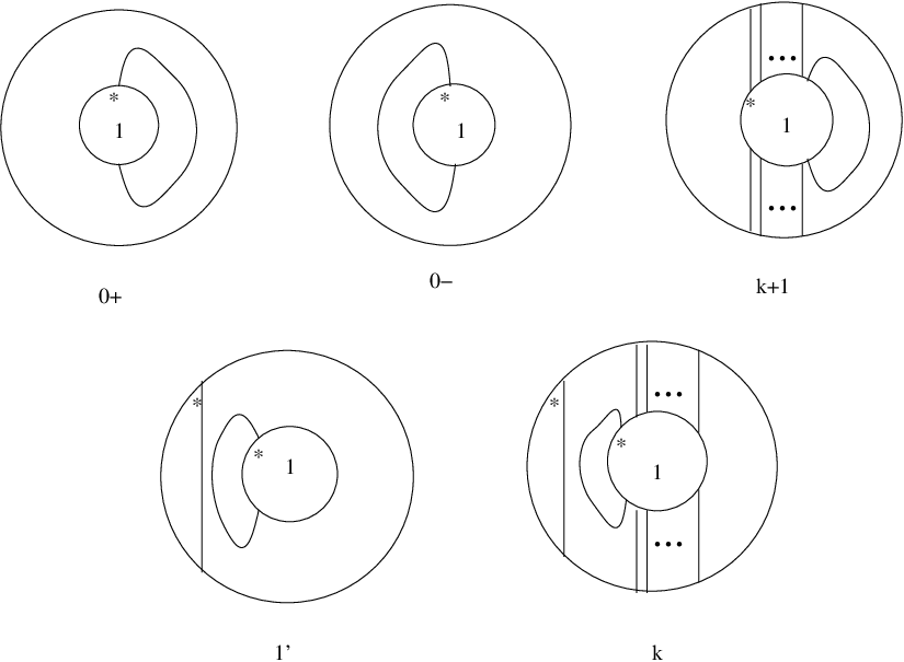

![[Uncaptioned image]](0806.1791v1/state.png)
![[Uncaptioned image]](0806.1791v1/singularity.png)
