Charge asymmetries in $\gamma\gamma\to\ell^{+}\ell^{-}+\nu$’s ($\ell=\mu,\,e$) with polarized photons in the Standard Model.

The Photon Collider (PC) option of the planned International Linear Collider (ILC) (see e.g. [1], [2]) will offer a specific window for the study of new effects in both Standard Model (SM) and New Physics. In particular, it is expected that the charge asymmetry of leptons, produced in the collision of neutral but highly polarized colliding particles $\gamma\gamma\to\ell^{+}\ell^{-}+neutrals$ (where $\ell=\mu,\,e$), can be a good tool for the discovery of New Physics effects. With this aim the study of such asymmetry in SM is a necessary step for both better knowledge of SM and understanding of background for New Physics effects.

In this paper we study the SM process, in which neutrals are neutrinos and the main (but not single) mechanism for charged lepton production is given by $\gamma\gamma\to W^{+}W^{-}$ process with subsequent lepton decay of $W$. The latter process, $\sigma(\gamma\gamma\to WW)Br(W\to\mu\nu)=8.8$ pb, will ensure very high event rate at the anticipated integrated luminosity of ILC (100 fb^-1), about $10^{6}$ events per year. The charge asymmetry here appears due to transformation of initial photon helicity into distribution of final leptons via P-violating but CP-preserving leptonic decay of $W$. In the following we consider the particular case ${\ell=\mu}$ for definiteness. The considered effects are identical for electrons and muons. So that, absolutely the same asymmetry will be observed in $e^{+}\,e^{-}$, $e^{+}\,\mu^{-}$, $\mu^{+}\,e^{-}$ distributions. All these contributions should be added for a complete analysis. This will enhance the value of the cross section for $\gamma\gamma\to\mu^{+}\mu^{-}+\nu^{\prime}s$ from 1.2 to 4.8 pb.

In the main body of the paper we consider the collision of a photon with helicity $\lambda_{1}$ moving in the positive direction of the $z$ axis with a photon of helicity $\lambda_{2}$ moving in the opposite direction. This initial state is denoted as $\gamma_{\lambda_{1}}\gamma_{\lambda_{2}}$ with $\lambda_{i}=\pm$ (left or right circular polarization). For example, the initial state with $\lambda_{1}=+1$, $\lambda_{2}=-1$ is written as $\gamma_{+}\gamma_{-}$. With this choice of the positive direction of the $z$ axis we define the longitudinal momentum $p_{\|}\equiv p_{z}$ and the transverse momentum $p_{\bot}\equiv\sqrt{p_{x}^{2}+p_{y}^{2}}$. For definiteness, we present most of the results for monochromatic photon beams at $\sqrt{s}_{\gamma\gamma}=500$ GeV ($E_{\gamma}=250$ GeV). The above definitions will be slightly modified when discussing the effects due to the non-monochromaticity of photon beams in the future Photon Collider. We start our numerical calculations with the CompHEP package [3] and then switch to the CalcHEP package [4] which allows one to take into account the circular polarization of the initial photons and choose different random seed numbers for the Monte Carlo (MC) generator which is necessary for an estimate of the statistical inaccuracy of future experiments.

The observable final state with $W+\mu$ or two muons with missing transverse momentum carried away by neutrinos can appear either via processes

or via cascade processes like:

in which six or eight particles are present in the final state.

To reduce CPU time in the Monte Carlo event generation, $10^{6}$ events for each channel, we obtain the essential part of the results for the $\mbox{$\gamma\gamma\,$}\to W^{\pm}\mu^{\mp}+\nu^{\prime}s$ process, not taking into account issues related to the reconstruction of the $W$. The analysis of this process allows us to extract the main features of the effect of interest, i.e. the difference in the distributions of $\mu^{+}$ and $\mu^{-}$ at fixed photon helicities (global charge asymmetry). We show that the additional diagrams that contribute to $\gamma\gamma\to\ell^{+}\ell^{-}+neutrals$ give negligible contribution to the cross section and charge asymmetry.

We start with the description in Section II of the general features of the effect, neglecting cascade processes. We classify the diagrams contributing to $\gamma\gamma\to W\mu\nu$ and $\gamma\gamma\to\mu^{+}\mu^{-}\nu_{\mu}\bar{\nu}_{\mu}$ according to the different topologies and give an approximate analytical estimate of their relative impact on the cross section (Sec. II.1). These estimates allow us to present qualitative explanation of the appearance of the charge asymmetry (Sec. II.2).

We then introduce suitable variables for the description of the global asymmetry, i.e. the difference in distributions of $\mu^{+}$ and $\mu^{-}$ in the processes $\gamma\gamma\to W^{\pm}\mu^{\pm}+\nu$’s or $\mbox{$\gamma\gamma\,$}\to\mu^{+}\mu^{-}+\nu$’s (Sec. II.4). In this very section we describe the cuts applied to the observed particles. In Sec. II.5 we discuss a computational method used to estimate a lower bound on the statistical uncertainty of future experiments. This estimate is obtained directly by the repeated Monte Carlo simulations with an anticipated number of events.

Section III is devoted to detailed description of the global charge asymmetry of leptons in the process $\mbox{$\gamma\gamma\,$}\to W\mu\nu$ in monochromatic $\gamma\gamma\,$ collisions.

The accurate calculation of cascade processes with six or more particles in the final state is a computationally challenging task with available software. Since we use CompHEP/CalcHEP packages which don’t fix the helicity of final states while the discussed effects strongly depend on the helicity, the direct use of existing software for tau decay simulation like TAUOLA [5] is not possible here. In Sec. IV we construct reasonable approximations in the description of cascade processes (3). The detailed analysis of the modification of momentum distributions allows to find that the inaccuracy implemented by the mentioned approximation in the final result is within the estimated statistical uncertainty of future experiments.

In Sec. V we discuss the total observable asymmetries.

High energy photons will be produced at the Photon Collider through Compton back-scattering of laser photons from high energy electron or (and) positron beams: the photons will not be monochromatic but will demonstrate an energy and polarization distribution. The high energy part of this spectrum will mainly include photons with definite helicity $\lambda_{i}$ close to $\pm 1$ [2]. We analyse the influence of initial photon non-monochromaticity on results in Sec. VI.

The correlative asymmetry in $\mu^{+}$ and $\mu^{-}$ momenta in each event of $\gamma\gamma\to\mu^{+}\mu^{-}+\nu^{\prime}s$ is expected to provide more information in the search for effects of physics beyond the SM. We discuss it in Sec. VII.

We conclude and summarize the obtained results in Sec. VIII.

Preliminary (and incomplete) parts of this work were reported earlier [6].

The SM cross section of $\gamma\gamma\to W^{+}W^{-}$ at center of mass energy greater than $200$ GeV remains almost constant at the asymptotic value $\sigma\simeq 8\pi\alpha^{2}/{M_{W}^{2}}\simeq 80$ pb and practically independent on photon polarization [8], see the formulas in Subsection II.2. At $\sqrt{s}>200$ GeV this cross section is more than ten times larger than the cross section of $W$ production in $e^{+}e^{-}\,$  mode. It will ensure very high event rate at the anticipated luminosity. The distributions of $W^{+}$ and $W^{-}$ bosons in $\gamma\gamma\to W^{+}W^{-}$ process are identical (charge symmetrical distribution), their polarizations are determined by the polarization of initial photons. The distribution of muons in subsequent decay of polarized $W^{\pm}$ is asymmetrical due to P non-conservation with CP conservation in the SM.

We start with the study of asymmetry neglecting the cascade channel and supposing photon beams monochromatic and completely polarized. First, we present the distributions $\partial^{2}\sigma/(\partial p_{\parallel}\partial p_{\perp})$ of muons in the ($p_{\|},\,p_{\bot}$) plane, at different photon polarizations, in Figs. 3. These figures show explicitly strong difference in the distributions of negative and positive muons as well as strong dependence of distributions on photon polarizations. Therefore, the charge asymmetry in the process is a strong effect.

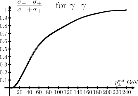
Table I presents obtained average momenta for the negative and positive muons and corresponding asymmetry quantities (7) together with their statistical uncertainties (in percents) for different cuts $p_{\bot\mu}^{c}$. One can see that the values of asymmetry are typically 20-50%.

We have checked that with the change of sign of both photon helicities mean muon momenta for negative and positive muons change their places (within statistical accuracy) so that the quantities $\Delta_{L,T}$ change their signs with this change of polarization.

The longitudinal scale of distributions in momenta is determined by initial photon energy while the transverse scale is determined by the $W$ mass. Hereupon mean transverse momenta are usually smaller than longitudinal.

Besides, for the collision of photons with identical helicity at the growth of cut $p_{\bot\mu}^{c}$ the cross sections for production of positive and negative muons become different, due to discussed charge asymmetry (remind, we discuss only events with negative muons or $W$’s flying in forward hemisphere). For the collision of photons with opposite helicity these cross sections should coincide since, for example, for $\gamma_{-}\gamma_{+}$ collision forward hemisphere for $\mu^{-}$ production realize absolutely the same distribution as backward hemisphere for $\mu^{+}$ production. This effect is clearly seen from Figure 4, where we present the $p_{\bot\mu}^{c}$ dependence for cross sections (13) at different initial photon polarizations.

The corresponding cross section differences, Eq. (12), are shown in Figure 5 without averaging over realizations. The difference in cross sections for $\gamma_{-}\gamma_{-}$ and $\gamma_{+}\gamma_{+}$ collisions is due to our choice of events with negative particles in forward hemisphere. In this case the cross sections coincide at small $p_{\bot\mu}^{c}$, while at high $p_{\bot\mu}^{c}$ one of them becomes larger and larger in comparison with the other, thus $\Delta\sigma$ goes to one (one more demonstration of transverse asymmetry). For the case with opposite photon helicities the deviation of $\Delta\sigma$ from zero shows high statistical uncertainty, due to the very low value of the cross sections (low counting rates) at $p_{\bot\mu}>120$ GeV. Similar dependencies with roughly the same characteristic values of $p_{\bot\mu}^{c}$ remain valid even at higher collision energies (for example, at $\sqrt{s}=2$ TeV) since the scale of this dependence is determined by the $W$ boson mass and not by the total energy.

The observable final state with two muons or $W+\mu$ with missing transverse momentum carried away by neutrinos can appear either via processes $\gamma\gamma\to\mu^{+}\mu^{-}\nu_{\mu}\bar{\nu}_{\mu}$ ($\gamma\gamma\to W\mu\nu$) or via cascade processes with $\tau$ production and subsequent $\tau$ decay ($\tau\to\mu\nu_{\mu}\nu_{\tau}$), see Eq.(3). The latter process enhances the total event rate (without cuts) by a value given by factor $B\equiv Br(\tau\to\mu\nu\nu)=17\,\%$ for the $\mbox{$\gamma\gamma\,$}\to W\mu+\nu^{\prime}s$. Similar event rate enhancement in the process $\mbox{$\gamma\gamma\,$}\to\mu^{+}\mu^{-}+\nu^{\prime}s$ is $2B+B^{2}\approx 37\,\%$.

The accurate calculation of processes with six or more particles in the final state like$\gamma\gamma\to\mu^{+}\mu^{-}\nu_{\mu}\bar{\nu}_{\mu}\nu_{\tau}\bar{\nu}_{\tau}$ is a computationally challenging task with available software. Since $\tau$ is very narrow particle, the diagrams without $\tau$-pole in $s$-channel can be neglected with very high precision, ($\sim\Gamma_{\tau}/m_{\tau}$). Therefore, one can in principle use the results for $\mbox{$\gamma\gamma\,$}\to W\tau\nu$ ($\gamma\gamma\to\tau^{+}\mu^{-}\nu_{\mu}\bar{\nu}_{\mu}$, etc.) and convolute them with the distribution of $\mu$ from $\tau$ decay. However, the latter distribution depends on $\tau$ polarization which cannot be determined definitely with CompHEP/CalcHEP in general case. (Generally, all helicity amplitudes for $\tau$ production are nonzero, and for convolution one must consider not only diagonal helicity states but also their interference).

Fortunately, the cascade process provides only a small fraction of the total cross section and the main contribution to the total cross section is given by the double resonant (DRD) diagrams of Fig. 1(a). That is the reason why in the description of the cascade contribution only these diagrams can be taken into account — DRD approximation. In this approximation the $\tau$ helicity is precisely determined in each MC event. In sect. V.1 we will show that the inaccuracy introduced in the total result using the DRD approximation for the cascade contribution is within the estimated statistical uncertainty, found for the main process.

Note that the distributions obtained in sect. III describe with high accuracy also $\tau$-distributions in $\mbox{$\gamma\gamma\,$}\to W\tau\nu$ processes etc.

In the DRD approximation each $\tau$ is produced only via $W$-decay, and its polarization in the rest frame of $W$ is given by the SM vertex, $\tau^{+}W^{-}_{\mu}\gamma^{\mu}(1-\gamma^{5})\nu_{\tau}+h.c.$. Due to $\gamma^{\mu}(1-\gamma^{5})$ factor, $\tau$ helicity is opposite to that of $\nu_{\tau}$, it is positive for $\tau^{+}$ and negative for $\tau^{-}$ (with accuracy to $m_{\tau}/M_{W}$) and independent on $W$ polarization.

For each generated event momenta of all particles are known. The spin vector of $\tau$ is expressed easily via momenta of $\tau$ and $\nu_{\tau}$, $p_{\tau}$ and $p_{\nu}$ respectively, as

Denoting the momentum of $\mu$ by $k$, the distribution of muons in $\tau$-decay with momentum $p_{\tau}$ and spin $\pm s$ can be written, neglecting muon mass, as

where $d\Gamma$ is a phase space element boosted to the lab frame. In the $\tau$ rest frame $d\Gamma=\theta\left(m_{\tau}/2-k\right)d^{3}k/E_{\mu}$. Note that the sign of helicity before $s$ in Eq. (14) disappears in the result.

Let us discuss now the qualitative features of the muon spectrum given by the convolution of the $\tau$ spectrum with the distribution in Eq. (15). One can consider $\tau\to\mu\nu\nu$ decay as a two body decay: a massless muon and the di-neutrino with invariant mass $m_{\nu\nu}$. At given $m_{\nu\nu}$, the energy and 3-momentum of the muon in the $\tau$ rest frame are ${\varepsilon}_{\mu}=p_{\mu}^{0}=Am_{\tau}/2$ with $A=1-(m_{\nu\nu}/m_{\tau})^{2}$. In the laboratory frame where the 3-momentum of the $\tau$, $\vec{p}_{\tau}$ is under some angle $\theta$ relative to muon momentum in $\tau$ rest frame, the muon momentum is evidently $\vec{p}_{\mu}=A\vec{p}_{\tau}(1+\cos\theta)/2$ plus small corrections negligible in our discussion. Therefore, the muon distribution repeats in some sense that of the $\tau$ but with a factor $A(1+\cos\theta)/2$, which is usually much lower than one. In other words, the distribution of muons in the cascade process is similar in the main features to that of the $\tau$ but it is strongly contracted to the origin of the coordinates.

$\bullet$ It is useful to describe the inaccuracy of the DRD approximation in the description of the $\mbox{$\gamma\gamma\,$}\to W\tau\nu$ cross section itself, $\delta^{\tau W}_{DRD}$, in dependence on the cut $p_{\bot\tau}^{c}$. The estimates in Sec. II.1 show that at the considered energies all contributions to the cross section are small in comparison with that of the DRD except for the SRDW contribution. The interference term $Re(A_{DRD}^{*}A_{SRDW})$ is roughly of the same order of magnitude as $|A_{SRDW}|^{2}$ since the DRD is large only in regions of the final phase space corresponding to the $W$ resonances, while the other contributions do not have these peaks. The numerical value of this inaccuracy is obtained by direct comparison of this cross section, calculated with all diagrams, and those for DRD diagrams with MC simulation.

At $p_{\bot\tau}^{c}=10$ GeV we find that for the $\mbox{$\gamma\gamma\,$}\to W\tau\nu$ process the SRDW contribution itself is about 5 % of the DRD one, and the interference of this contribution with DRD is destructive so that the DRD contribution differs from total cross section only by about 1%. This difference naturally grows with increasing values of $p_{\bot\tau}^{c}$.

More important for us is the inaccuracy of DRD approximation in the description of asymmetry quantities (7). Table 2 presents value of inaccuracy $\delta^{\tau W}_{DRD}(p_{\bot\tau}^{c})$ introduced by DRD approximation in the description of $\mbox{$\gamma\gamma\,$}\to W\tau\nu$ process at different cut values of $\tau$ transverse momenta $p_{\bot\tau}^{c}$.

Large values of the relative quantity $\delta_{T}^{(+-)}$ at large $p_{\bot\tau}^{c}$ appear in the case when the absolute value of $\Delta_{T}^{(+-)}$ is negligibly small. One can see that this inaccuracy grows with increasing the value of the cut, see Fig. 5. However with this increase also the fraction of cascade process within the total process becomes smaller and smaller (see discussion at the end of next section).

For the processes $\mbox{$\gamma\gamma\,$}\to\mu^{\pm}\tau^{\mp}\nu\nu$ and $\mbox{$\gamma\gamma\,$}\to\tau^{+}\tau^{-}\nu\nu$ the inaccuracies of DRD approximation are $\delta^{\tau\mu}_{DRD}(p_{\bot\tau}^{c})=\delta^{\tau W}_{DRD}(p_{\bot\tau}^{c})$ and $\delta^{\tau\tau}_{DRD}(p_{\bot\tau}^{c})=2\delta^{\tau W}_{DRD}(p_{\bot\tau}^{c})$.

The resulting distributions include the complete tree-level results of $\mbox{$\gamma\gamma\,$}\to W\mu\nu$ and DRD approximation for cascade contribution.

Figures 7 show the total observable distributions of muons, i.e. the sum of distributions of muons in $\mbox{$\gamma\gamma\,$}\to W\mu\nu$ and $\mbox{$\gamma\gamma\,$}\to W\tau\nu\to W\mu\nu\nu\nu$, and Table 3 presents the corresponding total asymmetry quantities for $p_{\bot\mu}^{c}=10$ GeV.

Comparison with Fig. 3 and Table I shows that the cascade process introduces a change in the shape of muons distribution only at small momenta and its contribution reduces the asymmetry parameters $\Delta_{L,T}$ in average by about 3 % only.

The plots in Fig. 8 show the dependence of asymmetries $\Delta_{L}$ and $\Delta_{T}$ on $p_{\bot\mu}^{c}$. The longitudinal charge asymmetry remains large even with large cuts, while the transverse charge asymmetry diminishes with $p_{\bot\mu}^{c}$ growth. In particular, for $\gamma_{+}\gamma_{-}$ collision at $p_{\bot\mu}^{c}\geq 120$ GeV the quantities $P_{T}^{+}$ and $P_{T}^{-}$ practically coincide, giving negligible $\Delta_{T}$, right plot, with naturally high statistical uncertainty in this small quantity.

The $p_{\bot\mu}^{c}$ dependence of resulting cross sections for different photon polarizations is shown in Fig. 9. The difference in curves for $(++)$ and $(--)$ initial states arise because of our charge asymmetric selection of events, with negative particles flying in the forward hemisphere (see Sec. II.4).

At the PC photons will be non-monochromatic with spectra peaked near the high energy limit $E_{\gamma}^{max}$. Moreover, due to the finite distance between the conversion point (CP) and the interaction point (IP) and also due to rescatterings of laser photons on electrons after the first collision, photon spectra are even non-factorizable. Fortunately in their high energy part, ($E_{\gamma}>E_{\gamma}^{max}/\sqrt{2}$), these spectra are factorizable with a high precision and these photons have a high degree of polarization. Moreover, the form of the effective spectra in this region is described with high accuracy with the aid of only one additional parameter, independent from the details of the experimental setup, while the polarization is the same as for pure Compton effect [10]. The luminosity of the Photon Collider is normalized for this very region only.

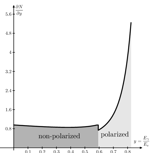
The low energy part of the effective photon spectrum, depends strongly on the details of the experimental setup which may change during the construction process of the ILC. Therefore, in our simulations, we used a photon spectrum composed of two parts as shown in Fig. 11. At $E_{\gamma}>E_{\gamma}^{max}/\sqrt{2}$ we used the approximation from Ref. [10] with $\rho=1$ and $x=4.8$ with polarization for ideal Compton effect [2]. In order to imitate the low energy part of the spectrum (at $E_{\gamma}<E_{\gamma}^{max}/\sqrt{2}$) we used spectra from [2] for the case when the IP and CP coincide ($\rho=0$) and consider these photons to be unpolarized.

In this section we denote by $\gamma_{-}$ an initial photon state obtained in collision of laser photon with helicity $P_{c}=+1$ and an electron with mean double initial helicity $2\lambda_{e}=0.85$, which gives $\lambda_{\gamma}=-1$ for photons with $E_{\gamma}=E_{\gamma}^{max}$. In this case mean polarization of photons with $E_{\gamma}>E_{\gamma}^{max}/\sqrt{2}$ is also negative but its absolute value is lower than one as it is described in [2]. At $E_{\gamma}<E_{\gamma}^{max}/\sqrt{2}$ we treat these photons as non-polarized. The state $\gamma_{+}$ is defined in the same way.

The resulting distributions of muons are presented on Fig. 12 for the case when incident electron energies are 250 GeV and the laser parameter is $x=4.8$. They resemble those presented in Fig. 3 with additional maximum at low energies. Table 4 shows the corresponding asymmetry quantities. These values are slightly smaller in comparison to the monochromatic case, but they are still large enough and replicate in main features the values in Table 1 with approximately the same statistical uncertainties.