Fixed points in models of continuous opinion dynamics under bounded confidence

Jan Lorenz ^†^†thanks: Email: post@janlo.de, present adress: ETH Zürich, Chair of Systems Design, Kreuzplatz˜5, 8032 Zürich, Switzerland Affiliation: Universität Bremen, Fachbereich Mathematik und Informatik Affiliation: Bibliothekstraße, 28359 Bremen, Germany Affiliation:

October 6, 2007

Abstract

We present two models of continuous opinion dynamics under bounded confidence which are representable as nonnegative discrete dynamical systems, namely the Hegselmann-Krause model (Hegselmann and Krause, Journal of Artificial Societies and Social Simulation 5(3), 2002) and the Deffuant-Weisbuch model (Deffuant et al, Advances in Complex Systems, 3, 2000). We fully characterize the set of fixed points for both models. They are identical. Further on, we present reformulations of both models on the more general level of densities of agents in the opinion space as interactive Markov chains. We also characterize the sets of fixed points as identical in both models.

agent-based models, density-based models, interactive Markov chain, discrete master equation

1 Introduction

Consider a set of $n\in\mathbb{N}$ agents which hold continuous opinions. ‘Continuous’ means that the opinion is in its essence a vector of $d\in\mathbb{N}$ real numbers. An example for a continuous opinion is a budget plan proposal, where a fixed amount of money is distributed to $d$ departements. Other examples are prices for products or an estimate of an unknown fact, like the number of humans on earth in 2050.

Consider further on that the agents are willing to adjust their opinion towards the opinions of others. Adjustment of a continuous opinion can be well described by computing a weighted arithmetic mean of other agent’s opinions. A process of continuous opinion dynamics can be seen as repeated averaging of opinions.

If the averaging weights are fixed (as in [8, 3, 4]) then the process can be mapped to $x(t+1)=Ax(t)$ with $x(0)$ being the $n$ -dimensional vector of opinions and $A$ being a row-stochastic matrix which represents the averaging weights for each agent in a row. The central research question was about conditions for reaching consensus.

Krause [13] invented a nonlinear bounded confidence model based on this linear model in 1997. Agents give positive weights to other agents only when they are close in opinion to their own opinion. So, agents may change their weights dynamically. Analytical conditions for convergence to consensus are only possible for very low number of agents [12], so in the next step extensive computer simulations have been done together with Hegselmann [11]. Then, the model got a lot of attention and is now mostly referenced as the Hegselmann-Krause model.

Independently, Deffuant and others invented a similar bounded confidence model working on a project [7, 6]about improving agri-environmental policies in 2000. Partly inspired by Axelrod [1] and particle physics they proposed a model of random pairwise interaction, where agents compromise if their opinions differ not too much.

Both models differ a lot in the detail (e.g. one is stochastic, one is deterministic) but are on the other hand similar in spirit, because they both make a ‘bounded confidence’-assumption for the agents. They can be represented as special cases in a general model [21]. For this general model it is possible to prove convergence to a limit opinion configuration [15]. But the proof does not use the bounded confidence assumption and nothing has been said about the set of all possible limit opinion configurations. This paper is to show the set of fixed points for both models (Section 2). Although the answer is quite plausible the proof for the Hegselmann-Krause model is not trivial.

Further on, both models have been redefined as density-based models. The idea goes back to Ben-Naim et al [2] in 2002 for the Deffuant-Weisbuch model and has been copied for the Hegselmann-Krause model [9]. Both can be approximated as state-discrete interactive Markov chains as done in [14, 16, 19] inspired by [5]. It has been seen in simulation that the density-based models also converge to limit opinion formations. Both types of limit formations are of the same heuristic type. But a proof of convergence is lacking.

This paper is furthermore to show the set of fixed points for the density-based models in their approxiamtion as interactive Markov chain (Section 3). Again the answer is quite plausible but the proof for the Hegselmann-Krause model is not trivial. The results for the fixed points of the interactive Markov chains are the central result of this paper.

In dynamical systems analysis it is natural to start finding the set of fixed points. Fixed points are stable opinion configurations. We guess that the processes in the agent-based as well as density-based model converge to one point in their set of fixed points. There is strong evidence from simulation for this conjecture, but a proof is lacking for the density-based models. As a starting point, we present a Lyapunov function which ensures that the density-based dynamics of the Deffuant-Weisbuch model can not have cycles.

The proofs for the fixed points of the interactive Markov chains rely on defining the difference equation which serves as a sort of discrete master equation which give gain and loss terms for each opinion class.

2 Agent-based bounded confidence models

Let us consider a set of $n\in\mathbb{N}$ agents which hold continuous opinions. An opinion is a real number or respectively a vector of $d\in\mathbb{N}$ real numbers. The opinion space is thus $S\subset\mathbb{R}^{d}$ . Usually $S$ is compact and convex. The opinion of agent $i\in\underline{n}$ at time $t\in\mathbb{N}$ is $x_{i}(t)\in S$ , and the vector $x(t)\in S^{n}$ is the opinion profile at time $t$ . Notice that $x(t)\in(\mathbb{R}^{d})^{n}$ is a vector of vectors for $d>1$ .

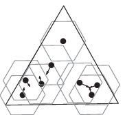
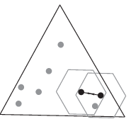
Figure 1 shows visualisations for the dynamics in one time step of both processes in a two dimensional triangular opinion space¹¹ 1 This opinion space could represent a simplex where opinions are proposals for the allocation of a fixed amount of money to three projects. See [17, 18] for simualtion results and the impact of the dimension in simplex opinion space.

Refer to caption — Figure 1: Visualisation for HK (left) and DW (right) dynamics in agent-based representation.

2.1 Agent-based Hegselmann-Krause model

Let there be $n\in\mathbb{N}$ agents and an appropriate opinion space $S\subset\mathbb{R}^{d}$ .

Given an initial profile $x(0)\in S^{n}$ , bound of confidence $\varepsilon>0$ and a norm $\left\|\cdot\right\|$ we define the HK process $(x(t))_{t\in\mathbb{N}}$ recursively through

x(t+1)=A(x(t),\varepsilon)x(t),

(1)

with $A(x,\varepsilon)$ being the confidence matrix defined

A_{ij}(x,\varepsilon):=\left\{\begin{array}[]{cl}\frac{1}{\#I_{\varepsilon}(i,x)}&\textrm{if }j\in I_{\varepsilon}(i,x)\\ 0&\textrm{otherwise,}\end{array}\right.\\

with $I_{\varepsilon}(i,x):=\{j\in\underline{n}\,|\,\left\|x^{i}-x^{j}\right\|\leq\varepsilon\}$ .

2.2 Agent-based Deffuant-Weisbuch model

Let there be $n\in\mathbb{N}$ agents and an opinion space $S\subset\mathbb{R}^{d}$ convex. Given an initial profile $x(0)\in S^{n}$ , bound of confidence $\varepsilon>0$ , and a norm $\left\|\cdot\right\|$ we define the DW process as the random process $(x(t))_{t\in\mathbb{N}}$ that chooses in each time step $t\in\mathbb{N}$ two random agents $i,j$ which perform the action

\displaystyle x^{i}(t+1)

\displaystyle=

\displaystyle\left\{\begin{array}[]{ll}\frac{1}{2}(x^{j}(t)+x^{i}(t))&\hbox{if $\left\|x^{i}(t)-x^{j}(t)\right\|\leq\varepsilon$}\\ x^{i}(t)&\hbox{otherwise.}\end{array}\right.

The same for $x^{j}(t+1)$ with $i$ and $j$ interchanged.

2.3 The set of fixed points in agent-based models

We call $x^{\ast}\in(\mathbb{R}^{d})^{n}$ a fixed point of the HK model if $A(x^{\ast},\varepsilon)x^{\ast}=x^{\ast}$ . We call $x^{\ast}\in(\mathbb{R}^{d})^{n}$ a fixed point of the DW model if for all choices $i,j\in\underline{n}$ the profile $x^{\ast}$ does not change if agents $i$ and $j$ communicate. Further, $F^{\mathrm{HK}}\subset(\mathbb{R}^{d})^{n}$ and $F^{\mathrm{DW}}\subset(\mathbb{R}^{d})^{n}$ are the sets of fixed points of the corresponding models.

In the following we describe these sets and show that they are equal. The proof for the DW model is trivial while the proof for the HK model needs a little bit of care. It relies on the finiteness of the number of agents.

The following lemma will be helpful. Beforehand we define for an opinion profile $x\in(\mathbb{R}^{d})^{n}$ and two agents $i,j\in\underline{n}$ as $H_{ij}\subset\mathbb{R}^{d}$ the hyperplane that is orthogonal to $x^{j}-x^{i}$ which goes through $x^{j}$ , and $H_{ij}^{+}\subset\mathbb{R}^{d}$ is the closed half-space defined by $H_{ij}$ which does not contain $x^{i}$ .

Lemma 1.

Let $x^{\ast}\in(\mathbb{R}^{d})^{n}$ be a fixed point of the homogeneous HK model with bound of confidence $\varepsilon>0$ . Let there be $i,j\in\underline{n}$ with $x^{i}\neq x^{j}$ such that $i\in I_{\varepsilon}(j,x)$ and let there be $k\in\underline{n}$ such that $x^{k}\not\in H_{ij}^{+}$ . Then there exists $m\in I_{\varepsilon}(j,x)$ different from $i,j,k$ such that $x^{m}\in H_{kj}^{+}$ .

Proof.

We abbreviate $x:=x^{\ast}$ . Due to $x$ being a fixed point it must hold that

x^{j}=\frac{1}{\#I_{\varepsilon}(j,x)}\sum_{s\in I_{\varepsilon}(j,x)}x^{s}.

So, $x^{j}$ is the barycenter of all the opinions in of agents in the confidence set $I_{\varepsilon}(j,x)$ . By definition $i\in I_{\varepsilon}(j,x)$ . Due to the fact that $k\not\in H_{ij}^{+}$ and that $H_{ij}^{+}$ is closed, the angle between $x^{i}-x^{j}$ and $x^{k}-x^{j}$ is less then $\frac{\pi}{2}$ and thus $i\not\in H_{kj}^{+}$ . (See Figure 2 for a visualisation.)

There must be at least one more agent in $I_{\varepsilon}(j,x)$ besides $i$ and $j$ , because otherwise $x^{j}$ is not the barycenter of $x^{i}$ and $x^{j}$ . If all these other agents were not in $H_{jk}^{+}$ then $x^{j}$ would be an extreme point²² 2 See Rockafellar [20] for convex analysis. of the convex hull of the opinions of the agents in $I_{\varepsilon}(j,x)$ . Thus, there must be $m\in I_{\varepsilon}(j,x)$ such that $x^{m}\in H_{jk}^{+}$ and $m\neq j$ . ∎

Proposition 2.

Let $\varepsilon>0$ be a bound of confidence which defines the homogeneous HK model and the DW model on the opinion space $(\mathbb{R}^{d})^{n}$ . It holds that

F^{\mathrm{HK}}=F^{\mathrm{DW}}=\{x\in(\mathbb{R}^{d})^{n}\,|\,\forall i,j\in\underline{n}:\left\|x^{i}-x^{j}\right\|_{p}>\varepsilon\hbox{ or }x^{i}=x^{j}\}.

(3)

Proof.

If $x$ is in the set as described in (3) each two agents either reached consensus or are too far away from each other to interact. Thus, $x$ is a fixed point in the DW and in the HK model.

Let $x$ be not in the set as described in (3) then there are $i,j\in\underline{n}$ such that $\left\|x^{i}-x^{j}\right\|_{p}\leq\varepsilon$ and $x^{i}\neq x^{j}$ .

Then $x$ can not be a fixed point of the DW model, because if $i,j$ are chosen as communication partners both agents will move towards each other.

It remains to show that $x$ cannot be a fixed point of the HK model. We assume that $x$ is a fixed point of the HK model and derive a contradiction.

Due to Lemma 1 there exists $m_{0}\in I_{\varepsilon}(j,x)$ with $x^{m_{0}}\in H_{ij}^{+}$ with

\left\|x^{i}-x^{m_{0}}\right\|_{2}>\left\|x^{i}-x^{j}\right\|_{2}

(we set $k$ in the lemma equal to $i$ ). Now we apply the lemma again for $j\in I_{\varepsilon}(m_{0},x)$ . Then obviously $i\not\in H_{jm_{0}}^{+}$ , and thus there is $m_{1}\in H_{im_{0}}^{+}$ such that $\left\|x^{i}-x^{m_{1}}\right\|_{2}>\left\|x^{i}-x^{m_{0}}\right\|_{2}$ . We can conclude like this to derive a sequence of agents $m_{0},m_{1},m_{2},\dots$ such that $\left\|x^{i}-x^{m_{0}}\right\|_{2}<\left\|x^{i}-x^{m_{1}}\right\|_{2}<\left\|x^{i}-x^{m_{2}}\right\|_{2}<\dots$ . This is a contradiction to the finiteness of the number of agents. ∎

Figure 3 gives impressions how the set of fixed points $F^{\mathrm{HK}}$ and $F^{\mathrm{DW}}$ looks for the opinion space $[0,1]\subset\mathbb{R}$ (so $d=1$ ), $n=2,3$ and $\varepsilon=0.3$ .

For higher $n$ (but still $d=1$ ) one can imagine this set like: Take the whole state space $\mathbb{R}^{n}$ and remove successively points. First, take all subspaces where numbers in two dimensions must be equal and remove the closed $\varepsilon$ -region around this subspaces from the whole space but keep the subspaces itself. Then take from every of these subspaces all subspaces where either a third number must be equal to the former two, or two other numbers must be equal and remove their $\varepsilon$ -region but keep the subspaces them self. Continuing like this spans a lattice of subspaces which is of the same kind as the lattice of partitions of the set $\{1,2,\dots,n\}$ . The number of subspaces to treat is much bigger than $n$ it is determined by the Bell numbers.

3 Density-based bounded confidence models

In the following we reformulate the Hegselmann-Krause model and Deffuant-Weisbuch model for a one-dimensional opinion space as density-based models with the same heuristics as in the agent-based model. We approximate density-based dynamics as interactive Markov chains as first outlined in [14].

Instead of concrete agents and their opinions we define the state of the system as a density function on the opinion space which evolves in time. As a simplification we only regard a one-dimensional interval as opinion space and discretise it into $n$ subintervals which serve as opinion classes. So, we switch from $n$ agents with opinions in the opinion space to an idealized infinite population, which is divided to the opinion classes $\underline{n}=\{1,\dots,n\}$ .

Class $i$ contains a fraction of the total population $p_{i}$ . For convenience we define $p_{i}=0$ for all $i\notin\underline{n}$ . A vector $p(t)\in\mathbb{R}^{n}$ represents the opinion distribution at time $t\in\mathbb{N}$ . Naturally, the fractions in the classes should sum up to one. So, the state space in a density-based model is a simplex. We define $\triangle^{n-1}=\{p\in\mathbb{R}^{n}_{\geq 0}\,|\,\sum_{i=1}^{n}p_{i}=1\}$ . One should think of an opinion distribution as a row vector.

If we define transition probabilities from one class to another we can represent the opinion dynamics process as an interactive Markov chain with transition matrix $B(p(t))$ . It is called ‘interactive’ because the transition matrix depends on the actual state of the system.

Let $\underline{n}$ be a set of opinion classes and $p(0)\in\triangle^{n-1}\subset\mathbb{R}^{n}$ be an initial opinion distribution. A density-based process is defined as an interactive Markov chain

p(t+1)=p(t)B(p(t))

(4)

with the explicit definition of the transition matrix function. In the following we give $B^{\mathrm{HK}}(p(t))$ for the HK model and $B^{\mathrm{DW}}(p(t))$ for the DW model.

3.1 Density-based Hegselmann-Krause transition matrix

We need some preliminary definitions to define the transition matrix for the interactive Markov chain with communication of repeated meetings like in the Hegselmann-Krause model.

Let $I=\{i,\stackrel{{\scriptstyle+1}}{{\dots}},j\}\subset\underline{n}$ be a discrete interval and $p\in\triangle^{n-1}$ be an opinion distribution. We call

M_{I}^{0}(p):=\sum_{k\in I}p_{k}\textrm{ the \emph{$I$-mass} (or 0th moment) of $p$,}

M_{I}^{1}(p):=\sum_{k\in I}kp_{k}\textrm{ the \emph{first $I$-moment} of $p$ and}

M_{I}^{\mathrm{bary}}(p):=\left\{\begin{array}[]{ll}\frac{M_{I}^{1}(p)}{M_{I}^{0}(p)},&\hbox{if $p_{I}\neq 0$,}\\ \frac{\max I+\min I}{2},&\hbox{if $p_{I}=0$.}\\ \end{array}\right.\textrm{ the \emph{$I$-barycenter} of $p$.}

Let $p\in\triangle^{n-1}$ be an opinion distribution and $\epsilon\in\mathbb{N}$ be a discrete bound of confidence. For $i\in\underline{n}$ we abbreviate the $\epsilon$ -local mean as

M_{i}:=M^{\mathrm{bary}}_{\{i-\epsilon,\stackrel{{\scriptstyle+1}}{{\dots}},i+\epsilon\}}(p)

We define the HK transition matrix as

B^{\mathrm{HK}}_{ij}(p,\epsilon):=\left\{\begin{array}[]{ll}1&\hbox{if $j=M_{i}$,}\\ \lceil M_{i}\rceil-M_{i}&\hbox{if $j=\lfloor M_{i}\rfloor$, $j\neq M_{i}$,}\\ M_{i}-\lfloor M_{i}\rfloor&\hbox{if $j=\lceil M_{i}\rceil$, $j\neq M_{i}$,}\\ 0&\hbox{otherwise.}\\ \end{array}\right.

Each row of the transition matrix $B^{\mathrm{HK}}(p,\epsilon)$ contains only one or two adjacent positive entries. The population with opinion $i$ goes completely to the $\epsilon$ -local mean opinion if this is an integer. Otherwise they distribute to the two adjacent opinions. The fraction which goes to the lower (upper) opinion class depends on how close the $\epsilon$ -local mean lies to it. Thus, the heuristic of averaging all opinions in a local area is represented. Figure 4 may give a hint how dynamics work.

3.2 Density-based Deffuant-Weisbuch transition matrix

The Deffuant-Weisbuch transition matrix for an opinion distribution $p\in\triangle^{n-1}$ , a discrete bound of confidence $\epsilon\in\mathbb{N}$ is defined by

B^{\mathrm{DW}}_{ij}(p,\epsilon,\mu)\left\{\begin{array}[]{ll}\frac{\pi^{i}_{2j-i-1}}{2}+\pi^{i}_{2j-i}+\frac{\pi^{i}_{2j-i+1}}{2},&\hbox{if $i\neq j$, }\\ q_{i},&\hbox{if $i=j$.}\\ \end{array}\right.

with $q_{i}=1-\sum_{j\neq i,j=1}^{n}B^{\mathrm{DW}}_{ij}(p,\epsilon,\mu)_{ij}$ and

\pi^{i}_{m}:=\left\{\begin{array}[]{ll}p_{m},&\hbox{if $|i-m|\leq\epsilon$}\\ 0,&\hbox{otherwise}\\ \end{array}\right.

Remember that we defined $p_{i}=0$ for all $i\not\in\underline{n}$ .

We briefly describe how the agent-based heuristics of the Deffuant-Weisbuch model governs the transition matrix of the interactive Markov chain. By the founding idea of the model an agent with opinion $i$ moves to the new opinion $j$ if he compromises with an agent with opinion $i+2(j-i)=2j-i$ . The probability to communicate with an agent with opinion $2j-i$ is of course $p_{2j-i}$ . Thus, the heuristic of random pairwise interaction is represented. The terms $\frac{\pi^{i}_{2j-i-1}}{2},\frac{\pi^{i}_{2j-i+1}}{2}$ stand for the case when agents with opinion $i$ communicate with agents with opinion $j$ , but the distance $|i-j|$ is odd. In this case the population should go with probability $\frac{1}{2}$ to one of the two possible opinion classes $\lfloor\frac{i+j}{2}\rfloor,\lceil\frac{i+j}{2}\rceil$ . Figure 4 may give a hint how dynamics work.

3.3 The set of fixed points in density based models

Here, we will prove that the set of fixed points of the interactive Markov chains

p(t+1)=p(t)B^{\mathrm{CR}}(p(t),\epsilon)

(5)

with DW and HK transition matrix is

G^{\mathrm{HK}}=G^{\mathrm{DW}}=\{p\in\triangle^{n-1}\,|\,p_{k}>0\Rightarrow p_{m}=0\textrm{ for all }m\in\{k-\epsilon,\stackrel{{\scriptstyle+1}}{{\dots}},k-2,k+2,\stackrel{{\scriptstyle+1}}{{\dots}},k+\epsilon\}\cap\underline{n}\}.

(6)

The structure of the set of fixed points is thus: all opinion classes with positive mass lie in adjacent pairs or isolated. Pairs and isolated classes must have a distance greater than $\epsilon$ to each other. In an adjacent pair of classes in a fixed point there are no further restrictions on the proportion of agents in the two classes. So, fixed points lie in certain lines in the simplex $\triangle^{n-1}$ .

Further on, we give a Lyapunov-function for the interactive Markov chain with DW transition matrix which rules out cycles. Convergence to fixed point remains as conjecture for the DW as well as for the HK transition matrix.

For both interactive Markov chains it is useful to look at their difference equation, because it can play the role of a discrete master equation (see [10]), which displays gain and loss terms for the mass changes in one class at one time step.

Let

\Delta p:=pB^{\mathrm{CR}}(p,\epsilon)-p=p(B^{\mathrm{CR}}(p,\epsilon)-E),

(7)

then the interactive Markov chain is a trajectory of the equation

p(t+1)=p(t)+\Delta p(t)=p(t)+p(t)(B^{\mathrm{CR}}(p(t),\epsilon)-E).

An opinion distribution $p^{\ast}$ is a fixed point of the interactive Markov chain (5) if $p^{\ast}=p^{\ast}B^{\mathrm{CR}}(p^{\ast},\epsilon)$ . Obviously, this is equivalent to $\Delta p^{\ast}=0$ .

3.3.1 The Deffuant-Weisbuch model

We take a look at the difference $\Delta p$ in detail. Simply calculating equation (7) with $B^{\mathrm{CR}}(p,\epsilon):=B^{\mathrm{DW}}(p,\epsilon)$ leads to the the following explanatory difference equation for all $k\in\underline{n}$ .

\Delta p_{k}=\underbrace{\sum_{\frac{i+j}{2}=k,2\leq|i-j|\leq\epsilon}p_{i}p_{j}+\sum_{\frac{i+j}{2}=k\pm\frac{1}{2},2\leq|i-j|\leq\epsilon}\frac{1}{2}p_{i}p_{j}}_{\textrm{fraction joining state $k$}}-\underbrace{p_{k}\sum_{2\leq|j-k|\leq\epsilon}p_{j}}_{\textrm{fraction leaving state $k$}}

(8)

(The first two sums go over all $(i,j)\in\underline{n}\times\underline{n}$ , the third over $j\in\underline{n}$ , under restriction of the equations below.) This is analog to a master equation in physics determining the fraction leaving a state and the fraction joining a state, but discrete in state and time.

Theorem 3.

An opinion distribution $p\in\triangle^{n-1}\subset\mathbb{R}^{n}$ is a fixed point of the interactive Markov chain (5) with DW transition matrix and discrete bound of confidence $\epsilon\in\mathbb{N}$ if and only if it holds for all $k\in\underline{n}$ that

p_{k}>0\Rightarrow p_{m}=0\textrm{ for all }m\in\{k-\epsilon,\stackrel{{\scriptstyle+1}}{{\dots}},k-2,k+2,\stackrel{{\scriptstyle+1}}{{\dots}},k+\epsilon\}\cap\underline{n}.

(9)

Proof.

For the ‘if’-part let us assume that $p$ is a fixed point and show that (9) holds. If $p$ is a fixed point it holds $\Delta p_{k}=0$ for all $k\in\underline{n}$ .

Let $k\in\underline{n}$ be such that $p_{k}>0$ . For an indirect proof let us assume that there is $m_{0}\in\{k-\epsilon,\dots,k-2,k+2,\dots,k+\epsilon\}\cap\underline{n}$ such that $p_{m_{0}}>0$ and find a contradiction.

We can conclude from $\Delta p_{k}=0$ and equation (8) that it holds

\underbrace{p_{k}}_{>0}\underbrace{\sum_{2\leq|j-k|\leq\epsilon}p_{j}}_{>0\textrm{ because it contains $p_{m_{0}}$}}=\sum_{\frac{i+j}{2}=k,2\leq|i-j|\leq\epsilon}p_{i}p_{j}+\sum_{\frac{i+j}{2}=k\pm\frac{1}{2},2\leq|i-j|\leq\epsilon}\frac{1}{2}p_{i}p_{j}

Thus, on the right hand side one addend $p_{m_{1}}p_{n_{1}}$ must be positive. A careful look at the summation index sets will help us to conclude further. If we assume without loss of generality $m_{1}<n_{1}$ then we can conclude $m_{1}<k$ .

We can conclude from $\Delta p^{\ast}_{m_{1}}=0$ and equation (8) that

\underbrace{p^{\ast}_{m_{1}}}_{>0}\underbrace{\sum_{2\leq|j-m_{1}|}p^{\ast}_{j}}_{>0\textrm{ because it contains $p^{\ast}_{n_{1}}$}}=\sum_{\frac{i+j}{2}=m_{1},2\leq|i-j|\leq\epsilon}p_{i}p_{j}+\sum_{\frac{i+j}{2}=m_{1}\pm\frac{1}{2},2\leq|i-j|\leq\epsilon}\frac{1}{2}p_{i}p_{j}

Thus, on the right hand side one addend $p_{m_{2}}p_{n_{2}}$ must be positive again and there is $m_{2}<m_{1}<k$ .

We conclude by induction until we reach an index $m_{z}<1$ for which $p_{m_{z}}$ must be positive – a contradiction.

To prove the ‘only if’-part we assume that for all $k\in\underline{n}$ it holds (9). We have to check that $\Delta p_{k}=0$ in equation (8) for all $k\in\underline{n}$ . We see that every addend in each equation is of the form $p_{i}p_{j}$ with $2\leq|j-l|\leq\epsilon$ and $\frac{i+j}{2}\in\{k,k\pm\frac{1}{2}\}$ . From (9) we know that in every case either $p_{i}$ or $p_{j}$ are zero. ∎

Theorem 4.

For every $p(0)\in\triangle^{n-1}\subset\mathbb{R}^{n}$ the interactive DW Markov chain $(p(t))_{t\in\mathbb{N}_{0}}$ can not be periodic.

Proof.

We define a Lyapunov function $L:S_{n}\to\mathbb{R}$ which is continuous and strictly decreasing on $(p(t))_{t\in\mathbb{N}_{0}}$ for every initial distribution $p(0)$ as long as we do not reach a fixed point. Let

L(p):=\sum_{i=1}^{n}2^{i}p_{i}.

Now we have to show that for every $p$ which is not a fixed point it holds that $L(p)>L(pB(p,\epsilon))$ .

Because of the linearity of $L$ we can transform the inequality such that we have to show

0>L(pB(p,\epsilon)-p)=L(\Delta(p)).

Due to (8) it holds

$\displaystyle L(\Delta p)$	$\displaystyle=$	$\displaystyle\sum_{k\in\underline{n}}2^{k}\left(\sum_{\frac{i+j}{2}=k,2\leq\|i-j\|\leq\epsilon}p_{i}p_{j}+\sum_{\frac{i+j}{2}=k\pm\frac{1}{2},2\leq\|i-j\|\leq\epsilon}\frac{1}{2}p_{i}p_{j}\right.$
		$\displaystyle\quad\quad\quad\quad\quad\quad\quad\quad\quad\quad\quad\quad\quad\left.-p_{k}\sum_{2\leq\|j-k\|\leq\epsilon}p_{j}\right)$
	$\displaystyle=$	$\displaystyle\sum_{2\leq\|i-j\|\leq\epsilon}(2^{\lfloor\frac{i+j}{2}\rfloor}+2^{\lceil\frac{i+j}{2}\rceil})p_{i}p_{j}+\sum_{2\leq\|i-j\|\leq\epsilon}(2^{i}+2^{j})p_{i}p_{j}$
	$\displaystyle=$	$\displaystyle\sum_{2\leq\|i-j\|\leq\epsilon}(2^{\lfloor\frac{i+j}{2}\rfloor}+2^{\lceil\frac{i+j}{2}\rceil}-2^{i}-2^{j})p_{i}p_{j}$

It holds $(2^{\lfloor\frac{i+j}{2}\rfloor}+2^{\lceil\frac{i+j}{2}\rceil}-2^{i}-2^{j})<0$ for all $i,j$ with $|i-j|\geq 2$ and thus it holds $L(\Delta p_{i})<0$ .

Due to the existence of the Lyapunov function it holds that $(p(t))_{t\in\mathbb{N}_{0}}$ can not have cycles. Because if we consider that there is a period $T\in\mathbb{N}$ such that $p(t)=p(t+T)$ then the sum $\sum_{s=t}^{t+T-1}L(\Delta p(s))$ would be negative, but on the other hand it also holds

\sum_{s=t}^{t+T}L(\Delta p(t))=\sum_{s=t}^{t+T}L(p(s+1)-p(s))=\sum_{s=t}^{t+T}L(p(s+1))-L(p(s))=0.

Thus there is a contradiction to a periodic solution. ∎

If one would define a Lyapunov function which is zero on every fixed point one might prove convergence to a fixed point.

Conjecture. For every $p(0)\in\triangle^{n-1}\subset\mathbb{R}^{n}$ the interactive DW Markov chain $(p(t))_{t\in\mathbb{N}_{0}}$ converges to a fixed point.

There is evidence from simulation for this conjecture [19].

3.3.2 The Hegselmann-Krause model

Here we show that the fixed points of the interactive Markov chain (4) with HK transition matrix are the same as for the DW transition matrix.

We start with a lemma on the $I$ -barycenters.

Lemma 5.

Let $p\in\triangle^{n-1}\subset R^{n}$ be an opinion distribution and discrete intervals $I_{0}=\{i_{0},\stackrel{{\scriptstyle+1}}{{\dots}},j_{0}\}\subset\underline{n}$ and $I_{1}=\{i_{1},\stackrel{{\scriptstyle+1}}{{\dots}},j_{1}\}\subset\underline{n}$ . It holds

1.

$i_{0}\leq i_{1}$ and $j_{0}\leq j_{1}\Longrightarrow M^{\mathrm{bary}}_{I_{0}}(p)\leq M^{\mathrm{bary}}_{I_{1}}(p),$

if $i_{0}\leq i_{1}$ and $j_{0}\leq j_{1}$

M^{\mathrm{bary}}_{I_{0}}(p)<M^{\mathrm{bary}}_{I_{1}}(p)\Longleftrightarrow\exists m\in(I_{0}\cup I_{1})\setminus(I_{0}\cap I_{1})\textrm{ with }p_{m}>0.

Proof.

In a first step we assume $p_{I_{0}}\neq 0$ and $p_{I_{1}}\neq 0$ Thus there is $m_{0}\in I_{0}$ with $p_{m_{0}}>0$ and one $m_{1}\in I_{1}$ with $p_{m_{1}}>0$ thus the following equation is well defined:

	$\displaystyle M^{\mathrm{bary}}_{I_{0}}(p)$	$\displaystyle=$	$\displaystyle\frac{M^{1}_{I_{0}}(p)}{M^{0}_{I_{0}}(p)}=\frac{M^{1}_{I_{0}}(p)M^{0}_{I_{1}}(p)}{M^{0}_{I_{0}}(p)M^{1}_{I_{1}}(p)}M^{\mathrm{bary}}_{I_{1}}(p)$
		$\displaystyle=$	$\displaystyle\frac{\sum\limits_{(m_{0},m_{1})\in I_{0}\times I_{1}}m_{0}p_{m_{0}}p_{m_{1}}}{\sum\limits_{(m_{0},m_{1})\in I_{0}\times I_{1}}m_{1}p_{m_{0}}p_{m_{1}}}M^{\mathrm{bary}}_{I_{1}}(p)$

To prove (1) we have to show that the fraction in equation (3.3.2) is less or equal than one.

We compare the summands in the numerator and the denominator. If $m_{0},m_{1}\in I_{0}\cap I_{1}$ then the summands $m_{0}p_{m_{0}}p_{m_{1}}$ and $m_{1}p_{m_{0}}p_{m_{1}}$ appear in both. In all other combination of indices it holds either $(m_{0},m_{1})\in(I_{0}\setminus I_{1})\times I_{1}$ or $(m_{0},m_{1})\in I_{0}\times(I_{1}\setminus I_{0})$ . Due to $i_{0}\leq i_{1}$ and $j_{0}\leq j_{1}$ it holds $m_{0}<m_{1}$ and thus the numerator is less or equal to the denominator and the fraction is less or equal to one.

To prove (2) we have to show that fraction in (3.3.2) is strictly less then one. This holds if there is a pair $(m_{0},m_{1})\in(I_{0}\setminus I_{1})\times I_{1}$ or $(m_{0},m_{1})\in I_{0}\times(I_{1}\setminus I_{0})$ for which $p_{m_{0}}>0$ and $p_{m_{1}}>0$ . This is obviously the case due to the claim in (2) and the assumption $p_{I_{0}}\neq 0$ and $p_{I_{1}}\neq 0$ .

At least we have to check the case, where $p_{I_{0}}=0$ or $p_{I_{1}}=0$ . The same steps as in Equation (3.3.2) lead with the definition of the local mean to the equations

$\displaystyle p_{I_{0}}\neq 0,p_{I_{1}}=0$	$\displaystyle\Rightarrow$	$\displaystyle M_{I_{0}}^{\mathrm{bc}}(p)=\frac{2\sum_{m\in I_{0}\setminus I_{1}}mp_{m}}{(j_{1}+i_{1})\sum_{m\in I_{0}\setminus I_{1}}p_{m}}M_{I_{1}}^{\mathrm{bc}}(p)$
$\displaystyle p_{I_{0}}=0,p_{I_{1}}\neq 0$	$\displaystyle\Rightarrow$	$\displaystyle M_{I_{0}}^{\mathrm{bc}}(p)=\frac{(j_{0}+i_{0})\sum_{m\in I_{1}\setminus I_{0}}p_{m}}{2\sum_{m\in I_{1}\setminus I_{0}}mp_{m}}M_{I_{1}}^{\mathrm{bc}}(p)$
$\displaystyle p_{I_{0}}=0,p_{I_{1}}=0$	$\displaystyle\Rightarrow$	$\displaystyle M_{I_{0}}^{\mathrm{bc}}(p)=\frac{j_{0}+i_{0}}{j_{1}+i_{1}}M_{I_{1}}^{\mathrm{bc}}(p)$

(We can choose the summation index sets $I_{0}\setminus I_{1}$ instead of $I_{0}$ in the upper equation, because all summands with indices out of $I_{0}\cap I_{1}$ are obviously zero. Analog for the middle equation.) For all three equations we can conclude like above to get 1 and 2. ∎

For an opinion distribution $p\in\triangle^{n-1}\subset\mathbb{R}^{n}$ and a discrete bound of confidence $\epsilon\in\underline{n}$ we recall the abbreviation $M_{i}:=M^{\mathrm{bary}}_{\{i-\epsilon,\stackrel{{\scriptstyle+1}}{{\dots}},i+\epsilon\}}(p)$ . Due to Lemma 5 it holds

M_{1}\leq M_{2}\leq\dots\leq M_{n}.

(10)

Analog to the former subsection we reformulate (7), which leads to the following explanatory difference equation for all $k\in\underline{n}$ (again in analogy to a master equation).

\Delta p_{k}=\underbrace{\sum_{j\in I_{k}^{\lceil\cdot\rceil}}(M_{j}-\lfloor M_{j}\rfloor)p_{j}+\sum_{j\in I_{k}}p_{j}+\sum_{j\in I_{i}^{\lfloor\cdot\rfloor}}(\lceil M_{j}\rceil-M_{j})p_{j}}_{\textrm{fraction joining $k$}}\underbrace{-p_{k}}_{\textrm{fraction leaving $k$}}

(11)

with

I_{k}^{\lceil\cdot\rceil}:=\{j\in\underline{n}\,|\,M_{j}\neq k=\lceil M_{j}\rceil\textrm{ and }p_{k}>0\},

I_{k}^{\ast}:=\{j\in\underline{n}\,|\,k=M_{j}\textrm{ and }p_{k}>0\}\textrm{ and }

I_{k}^{\lfloor\cdot\rfloor}:=\{j\in\underline{n}\,|\,M_{j}\neq k=\lfloor M_{j}\rfloor\textrm{ and }p_{j}k>0\}.

It is easy to see with (10) that the sets $I_{i}^{\lceil\cdot\rceil},I_{i}^{\ast}$ and $I_{i}^{\lfloor\cdot\rfloor}$ are all discrete intervals, that they are pairwise disjoint and that their union

I_{i}:=I_{i}^{\lceil\cdot\rceil}\cup I_{i}^{\ast}\cup I_{i}^{\lfloor\cdot\rfloor}

is a discrete interval, too. We know also that the coefficients $(M_{j}-\lfloor M_{j}\rfloor)$ and $(\lceil M_{j}\rceil-M_{j})$ in (11) are always positive and strictly less than one by definition.

The following proposition shows that an opinion class with positive mass has a local barycenter which is less than one class away and that the adjacent class has positive mass too and a local barycenter between the two classes.

Proposition 6.

Let $p\in\triangle^{n-1}\subset\mathbb{R}^{n}$ be a fixed point of the interactive HK Markov chain (5) with HK transition matrix and let $p_{i}>0$ then it holds

	either		$\displaystyle M_{i}=i\textrm{ and }I_{i}=\{i\}$
	or		$\displaystyle i<M_{i}\leq M_{i+1}<i+1,p_{i+1}>0\textrm{ and }I_{i}=\{i,i+1\}=I_{i+1},$
	or		$\displaystyle i-1<M_{i-1}\leq M_{i}<i,p_{i-1}>0\textrm{ and }I_{i}=\{i,i-1\}=I_{i-1}$

Proof.

We define $p=[p_{1}\dots p_{n}]$ .

In a first step we will show that $i-1<M_{i}<i+1$ . Let us assume for an indirect proof that $M_{i}\geq i+1$ .

The fact that $p$ is a fixed point implies $\Delta p=0$ and thus we can derive from Equation (11) that

p_{i}=\sum_{j\in I_{i}^{\lceil\cdot\rceil}}(M_{j}-\lfloor M_{j}\rfloor)p_{j}+\sum_{j\in I_{i}^{\ast}}p_{j}+\sum_{j\in I_{i}^{\lfloor\cdot\rfloor}}(\lceil M_{j}\rceil-M_{j})p_{j}

(12)

Due to $M_{i}\geq i+1$ it holds that $i\not\in I_{i}$ (the union of all index sets) and due to Lemma 5 it holds for $j\in I_{i}$ that $j\leq i-1$ . Let $i_{1}:=\max I_{i}$ . Thus it is clear that $i_{1}<i,p_{i_{1}}>0$ and $i_{1}<M_{i_{1}}$ .

We conclude further with Equation (11) that

p_{i_{1}}=\sum_{j\in I_{i_{1}}^{\lceil\cdot\rceil}}(M_{j}-\lfloor M_{j}\rfloor)p_{j}+\sum_{j\in I_{i_{1}}^{\ast}}p_{j}+\sum_{j\in I_{i_{1}}^{\lfloor\cdot\rfloor}}(\lceil M_{j}\rceil-M_{j})p_{j}

(13)

It may $i_{1}\in I_{i_{1}}^{\lceil\cdot\rceil}$ but it holds $\max I_{i_{1}}\leq i_{1}$ and due to $(M_{j}-\lfloor M_{j}\rfloor)<1$ it holds that there must exist $i_{2}:=\max I_{i_{1}}\setminus\{i_{1}\}$ with $p_{i_{2}}>0$ and $i_{2}<M_{i_{2}}$ .

We derive by induction further on the existence of a decreasing chain of indices $i>i_{1}>i_{2}>\dots$ with $p_{i}>0,p_{i_{1}}>0,p_{i_{2}}>0,\dots$ . Thus there must be $z<1$ with $p_{z}>0$ , a contradiction, thus $M_{i}<i+1$ .

If we assume $M_{i}\leq i-1$ we can derive analog that there must be $z>n$ with $p_{z}>0$ . Thus we know $i-1<M_{i}<i+1$ .

In the second step we show $M_{i}>i\Rightarrow M_{i+1}<i+1,p_{i+1}>0$ . It is clear by Lemma 5 that $M_{i+1}\geq M_{i}$ , lets assume $M_{i+1}\geq i+1$ . Then we find (looking at Equation (12)) that $i\in I_{i}^{\lfloor\cdot\rfloor}$ and $i+1\not\in I_{i}$ thus we can conclude in the same way as after Equation (13) that there exist $z<1$ with $p_{z}>0$ . Thus it follows by this contradiction that $M_{i+1}<i+1$ . Analog we derive $M_{i}<i\Rightarrow M_{i-1}>i-1$

In the third step we show that $M_{i}>i$ implies $I_{i}=\{i,i+1\}=I_{i+1}$ and $p_{i+1}>0$ . From equation $\Delta p=0$ and Equation (11) we can derive the two equations

	$\displaystyle p_{i}$	$\displaystyle=$	$\displaystyle(\lceil M_{i}\rceil-M_{i})p_{i}+(\lceil M_{i+1}\rceil-M_{i+1})p_{i+1}+\sum_{j\in I_{i}\setminus\{i,i+1\}}\textrm{positive terms}$
	$\displaystyle p_{i+1}$	$\displaystyle=$	$\displaystyle(M_{i}-\lfloor M_{i}\rfloor)p_{i}+(M_{i+1}-\lfloor M_{i+1}\rfloor)p_{i+1}+\sum_{j\in I_{i+1}\setminus\{i,i+1\}}\textrm{positive terms}$

If we add both equations we get by calculation

0=\sum_{j\in I_{i}\setminus\{i,i+1\}}\textrm{positive terms}=\sum_{j\in I_{i+1}\setminus\{i,i+1\}}\textrm{positive terms}

and thus $I_{i}\setminus\{i,i+1\}$ and $I_{i+1}\setminus\{i,i+1\}$ must be empty. And due $i+1\in I_{i}$ it holds $p_{i+1}>0$ .

Analog, we prove that $M_{i}<i$ implies $I_{i}=\{i-1,i\}=I_{i-1}$ and $p_{i-1}>0$ . ∎

So, for the fixed point $p$ and $p_{i}>0$ we know that either $I_{i}=\{i\}$ or $I_{i}=\{i,i+1\}$ with $p_{i+1}>0$ or $I_{i}=\{i-1,i\}$ with $p_{i-1}>0$ . We define two new discrete intervals

I_{i}^{-\epsilon}:=\{(\min I_{i})-\epsilon,\stackrel{{\scriptstyle+1}}{{\dots}},(\min I_{i})-1\},

I_{i}^{+\epsilon}:=\{(\max I_{i})+1,\stackrel{{\scriptstyle+1}}{{\dots}},(\max I_{i})+\epsilon\}.

The discrete interval $I_{i}^{-\epsilon}\cup I_{i}\cup I_{i}^{+\epsilon}$ is the interval which contains all the classes where the imaginary agents in the classes of $I_{i}$ interact with. The next proposition shows that the class(es) in $I_{i}^{-\epsilon}$ and $I_{i}^{+\epsilon}$ can only both contain mass or both contain no mass.

Proposition 7.

Let $p\in\triangle^{n-1}\subset\mathbb{R}^{n}$ be a fixed point of the interactive HK Markov chain (5) with HK transition matrix and let $p_{i}>0$ then it holds

p_{I_{i}^{-\epsilon}}=0\Leftrightarrow p_{I_{i}^{+\epsilon}}=0.

Proof.

First we consider $I_{i}=\{i,i+1\}$ . Thus, due to Proposition 6 it holds $i<M_{i}\leq M_{i+1}<i+1$ . It holds $\Delta p=0$ because $p$ is a fixed point. From (11) we can thus derive

p_{i}=(\lceil M_{i}\rceil-M_{i})p_{i}+(\lceil M_{i+1}\rceil-M_{i+1})p_{i+1}

With $\lceil M_{i}\rceil=\lceil M_{i+1}\rceil=i+1$ it follows

p_{i}=((i+1)-M_{i})p_{i}+((i+1)-M_{i+1})p_{i+1}.

This can be transformed to

M_{i}p_{i}+M_{i+1}p_{i+1}=ip_{i}+(i+1)p_{i+1}

(14)

Now, we assume for an indirect proof that $p_{I_{i}^{-\epsilon}}=0$ and $p_{I_{i}^{+\epsilon}}\neq 0$ and derive a contradiction. Due to this assumption it holds $M_{i}=M^{\mathrm{bary}}_{\{i,\stackrel{{\scriptstyle+1}}{{\dots}},i+\epsilon\}}$ and $M_{i+1}=M^{\mathrm{bary}}_{\{i,\stackrel{{\scriptstyle+1}}{{\dots}},i+1+\epsilon\}}$ . Then it follows from lemma 5 that $M^{\mathrm{bary}}_{\{i,i+1\}}<M_{i+1}$ and $M^{\mathrm{bary}}_{\{i,i+1\}}\leq M_{i}$ . Now, we conclude from (14) that

M^{\mathrm{bary}}_{\{i,i+1\}}p_{i}+M^{\mathrm{bary}}_{\{i,i+1\}}p_{i+1}<ip_{i}+(i+1)p_{i+1}.

Both sides divided by the positive term $(p_{i}+p_{i+1})$ delivers

M^{\mathrm{bary}}_{\{i,i+1\}}<\frac{ip_{i}+(i+1)p_{i+1}}{p_{i}+p_{i+1}}=M^{\mathrm{bary}}_{\{i,i+1\}}.

A similar contradiction can be derived for the assumption $p_{I_{i}^{-\epsilon}}\neq 0$ and $p_{I_{i}^{+\epsilon}}=0$ . This proves $p_{I_{i}^{-\epsilon}}=0\Leftrightarrow p_{I_{i}^{+\epsilon}}=0$ .

For $I_{i}=\{i-1,i\}$ arguments are the same after renumbering $i\to i-1$ .

For $I_{i}=\{i\}$ it holds $M_{i}=i$ . Again, we assume for an indirect proof that $p_{I_{i}^{-\epsilon}}=0$ and $p_{I_{i}^{+\epsilon}}>0$ and derive a contradiction:

M_{i}=M^{\mathrm{bary}}_{\{i,\stackrel{{\scriptstyle+1}}{{\dots}},i+\epsilon\}}<M^{\mathrm{bary}}_{\{i\}}=i=M_{i}.

∎

Now, we show that the set of fixed points of the interactive Markov chain with HK transition matrix is the same as for the DW transition matrix.

Theorem 8.

An opinion distribution $p\in\triangle^{n-1}\subset\mathbb{R}^{n}$ is a fixed point of the interactive Markov chain (5) with HK transition matrix and discrete bound of confidence $\epsilon\in\mathbb{N}$ if and only if it holds for all $k\in\underline{n}$ that

p_{k}>0\Rightarrow p_{m}=0\textrm{ for all }m\in\{k-\epsilon,\dots,k-2,k+2,\dots,k+\epsilon\}\cap\underline{n}.

(15)

Proof.

For the ‘if’-part let us assume that $p$ is a fixed point and show that (15) holds. For an indirect proof we assume that there are $i,j\in\underline{n}$ such that $i<j$ , $2\leq|i-j|\leq\epsilon$ and $p_{i},p_{j}>0$ and find a contradiction.

From Proposition 6 we know that $I_{i}$ and $I_{j}$ are disjoint. From Proposition 7 we know that there must exist $m_{0}\in\mathbb{N}$ such that $m_{0}<i$ , $|i-m_{0}|\leq\epsilon$ , $p_{m_{0}}>0$ and $I_{m_{0}}$ and $I_{i}$ are disjoint. Comparing $m_{0}$ and $i$ we know with the same arguments that there must exist $m_{1}\in\mathbb{N}$ with $m_{1}<m_{0}$ , $|m_{0}-m_{1}|\leq\epsilon$ , $p_{m_{1}}>0$ and $I_{m_{1}}$ and $I_{m_{0}}$ are disjoint. By induction we can construct a sequence of natural numbers $m_{0}>m_{1}>m_{2}>\dots$ with $p_{m_{0}},p_{m_{1}},p_{m_{2}},\dots>0$ . Thus there must exist $z\in\mathbb{N}$ such that $m_{z}<1$ and $p_{m_{z}}>0$ , which is a contradiction.

To prove the ‘only if’-part we assume that for all $k\in\underline{n}$ it holds (15). We have to check that $\Delta p_{i}=0$ in (11) for all $i\in\underline{n}$ . We see that every addend in each equation is of the form $p_{i}p_{j}$ with $2\leq|j-l|\leq\epsilon$ and $\frac{i+j}{2}\in\{k,k\pm\frac{1}{2}\}$ . From (15) we know that in every case either $p_{i}$ or $p_{j}$ are zero. ∎

The convergence to a fixed point remains as a conjecture.

Conjecture. For every $p(0)\in\triangle^{n-1}\subset\mathbb{R}^{n}$ the interactive HK Markov chain $(p(t))_{t\in\mathbb{N}_{0}}$ converges to a fixed point. Convergence occurs in finite time.

There is strong evidence from simulation for the conjecture [19].

4 Conclusion

We characterised the set of fixed points for the agent-based DW and HK model. They are identical. We did the same for their corresponding density-based model versions (in the approximation of an interactive Markov chain).

The proofs were not in every case trivial (especially in the density-based HK model) although the set of fixed-points is quite plausible on a first view. One reason for this is that there can be arbitrary long covergence times in the HK model (for examples see [19]).

Proofs of convergence for the interactive Markov chains are still lacking, although there is strong evidence from simulation for convergence to one point in the set of fixed points. Further on, this is an interesting type of set convergence. The processe processes show an interesting type of set-convergence. In contrast to many other models these models have a huge amount of fixed points and more over they are not isolated but appear in lines, planes and hyperplanes. On the other hands in contrast to other types of set-convergence the process always converges to one of these fixed points and there are no limit cycles.

A last question is about a class of models for which one can prove that they have the presented sets of fixed points where both models appear as special cases. Here, proofs for both models have been derived seperately, although the models are similar in spirit.

References

[1] Robert Axelrod. The Dissemination of Culture: A Model with Local Convergnance and Global Polarization. Journal of Conflict Resolution, 41(203), 1997. reprinted in R. Axelrod, The complexity of cooperation, Princeton University Press, Princeton, 1997.
[2] Eli Ben-Naim, Sidney Redner, and Paul L. Krapivsky. Bifurcation and Patterns in Compromise Processes. Physica D, 183:190–204, 2003.
[3] Roger L. Berger. A Necessary and Sufficient Condition for Reaching Consensus Using DeGroot’s Method. Journal of the American Statistical Association, 76:415–418, 1981.
[4] Samprit Chatterjee and Eugene Seneta. Towards Consensus: Some Convergence Theorems on Repeated Averaging. J. Appl. Prob., 14:159–164, 1977.
[5] John Conlisk. Interactive Markov Chains. Journal of Mathematical Sociology, 4:157–185, 1976.
[6] Guillaume Deffuant, David Neau, Frédéric. Amblard, and Gérard Weisbuch. Mixing Beliefs among Interacting Agents. Advances in Complex Systems, 3:87–98, 2000.
[7] Guillaume Deffuant (Coordinator). Final report: Improving Agri-environmental Policies: a Simulation Approach to the Cognitive Properties of Farmers and Institutions (IMAGES). Technical report, EU Project: FAIR3 CT 2092, 2001.
[8] Morris H. DeGroot. Reaching a Consensus. Journal of the American Statistical Association, 69(345):118–121, 1974.
[9] Santo Fortunato, Vito Latora, Alessandro Pluchino, and Andrea Rapisarda. Vector Opinion Dynamics in a Bounded Confidence Consensus Model. International Journal of Modern Physics C, 16(10):1535–1551, 2005.
[10] Daniel T. Gillespie. Markov Processes - An Introduction for the Physical Scientist. Academic Press, Inc., 1992.
[11] Rainer Hegselmann and Ulrich Krause. Opinion Dynamics and Bounded Confidence, Models, Analysis and Simulation. Journal of Artificial Societies and Social Simulation, 5(3), 2002.
[12] Ulrich Krause. A Discrete Nonlinear and Non-Autonomous Model of Consensus Formation. In S. Elyadi, G. Ladas, J. Popenda, and J. Rakowski, editors, Communications in Difference Equations, pages 227–236. Gordon and Breach Pub., Amsterdam, 2000.
[13] Ulrich Krause and Manfred Stöckler, editors. Modellierung und Simulation von Dynamiken mit Vielen Interagierenden Akteuren. Modus, Universität Bremen, 1997.
[14] Jan Lorenz. Continuous Opinion Dynamics: Insights through Interactive Markov Chains;. Proceedings of IASTED Conference ”Modelling, Simulation and Optimization MSO 2005 ” August 29-31, Oranjestad, Aruba, 2005.
[15] Jan Lorenz. A Stabilization Theorem for Dynamics of Continuous Opinions. Physica A, 355(1):217–223, 2005.
[16] Jan Lorenz. Consensus Strikes Back in the Hegselmann-Krause Model of Continuous Opinion Dynamics under Bounded Confidence. Journal of Artificial Societies and Social Simulation, 9(1), 2006.
[17] Jan Lorenz. Continuous Opinion Dynamics of Multidimensional Allocation Problems under Bounded Confidence: More Dimensions Lead to Better Chances for Consensus. European Journal of Economic and Social Systems, 19:213–227, 2006.
[18] Jan Lorenz. Managing Complexity, Editor Dirk Helbing, chapter Fostering Consensus in Multidimensional Continuous Opinion Dynamics under bounded Confidence. Springer, 2007.
[19] Jan Lorenz. Repeated Averaging and Bounded Confidence – Modeling, Analysis and Simulation of Continuous Opinion Dynamics. PhD thesis, Universität Bremen, March 2007. http://nbn-resolving.de/urn:nbn:de:gbv:46-diss000106688.
[20] R. Tyrell Rockafellar. Convex Analysis. Princeton Landmarks in Mathematics. Princeton University Press, New Jersey, 1970.
[21] Diemo Urbig, Jan Lorenz, and Heiko Herzberg. Opinion Dynamics: the Effect of the Number of Peers Met at Once. Journal of Artificial Societies and Social Simulation, 11(2):4, 2008.