跳到论文正文
W Papers独立论文阅读器 arXiv:0806.1528 论文正文 计算阅读时间 · 0%
引用这篇论文根据当前论文元数据生成,正式投稿前建议核对。


License: arXiv.org perpetual non-exclusive license
arXiv:0806.1528v1 [math.SP] 09 Jun 2008
\urladdr

http://www.math.caltech.edu/people/simon.html

The Christoffel–Darboux Kernel

This work was supported in part by NSF grant DMS-0652919 and U.S.–Israel Binational Science Foundation (BSF) Grant No. 2002068
Barry Simon∗ Address: Mathematics 253–37, California Institute of Technology, Pasadena, CA 91125, U.S.A. Email: bsimon@caltech.edu
Abstract.

A review of the uses of the CD kernel in the spectral theory of orthogonal polynomials, concentrating on recent results.

keywords
Orthogonal polynomials, spectral theory
2000 Mathematics Subject Classification
34L40, 47-02, 42C05

1. Introduction

This article reviews a particular tool of the spectral theory of orthogonal polynomials. Let μ\mu be a measure on ℂ{\mathbb{C}} with finite moments, that is,

∫|z|n​𝑑μ​(z)<∞\int\lvert z\rvert^{n}\,d\mu(z)<\infty (1.1)

for all n=0,1,2,…n=0,1,2,\dots and which is nontrivial in the sense that it is not supported on a finite set of points. Thus, {zn}n=0∞\{z^{n}\}_{n=0}^{\infty} are independent in L2​(ℂ,d​μ)L^{2}({\mathbb{C}},d\mu), so by Gram–Schmidt, one can define monic orthogonal polynomials, Xn​(z,d​μ)X_{n}(z;d\mu), and orthonormal polynomials, xn=Xn/∥Xn∥L2x_{n}=X_{n}/\lVert X_{n}\rVert_{L^{2}}. Thus,

∫z¯j​Xn​(z,𝑑μ)​𝑑μ​(z)=0j=0,…,n−1\displaystyle\int\bar{z}^{j}X_{n}(z;d\mu)\,d\mu(z)=0\qquad j=0,\dots,n-1 (1.2)
Xn​(z)=zn+lower order\displaystyle X_{n}(z)=z^{n}+\text{lower order} (1.3)
∫xn​(z)¯​xm​(z)​𝑑μ=δn​m\displaystyle\int\overline{x_{n}(z)}\,x_{m}(z)\,d\mu=\delta_{nm} (1.4)

We will often be interested in the special cases where μ\mu is supported on ℝ{\mathbb{R}} (especially with support compact), in which case we use Pn,pnP_{n},p_{n} rather than Xn,xnX_{n},x_{n}, and where μ\mu is supported on ∂𝔻\partial{\mathbb{D}} (𝔻={z∣|z|<1}{\mathbb{D}}=\{z\mid\lvert z\rvert<1\}), in which case we use Φn,φn\Phi_{n},\varphi_{n}. We call these OPRL and OPUC (for “real line” and “unit circle”).

OPRL and OPUC are spectral theoretic because there are Jacobi parameters {an,bn}n=1∞\{a_{n},b_{n}\}_{n=1}^{\infty} and Verblunsky coefficients {αn}n=0∞\{\alpha_{n}\}_{n=0}^{\infty} with recursion relations (p−1=0p_{-1}=0; p0=Φ0=1p_{0}=\Phi_{0}=1):

z​pn​(z)\displaystyle zp_{n}(z) =an+1​pn+1​(z)+bn+1​pn​(z)+an​pn−1​(z)\displaystyle=a_{n+1}p_{n+1}(z)+b_{n+1}p_{n}(z)+a_{n}p_{n-1}(z) (1.5)
Φn+1​(z)\displaystyle\Phi_{n+1}(z) =z​Φn​(z)−α¯n​Φn∗​(z)\displaystyle=z\Phi_{n}(z)-\bar{\alpha}_{n}\Phi_{n}^{*}(z) (1.6)
Φn∗​(z)\displaystyle\Phi_{n}^{*}(z) =zn​Φn​(1/z¯)¯\displaystyle=z^{n}\,\overline{\Phi_{n}(1/\bar{z})} (1.7)

We will sometimes need the monic OPRL and normalized OPUC recursion relations:

z​Pn​(z)=Pn+1​(z)+bn+1​Pn​(z)+an2​Pn−1​(z)\displaystyle zP_{n}(z)=P_{n+1}(z)+b_{n+1}P_{n}(z)+a_{n}^{2}P_{n-1}(z) (1.8)
z​φn​(z)=ρn​φn+1​(z)+α¯n​φn∗​(z)\displaystyle z\varphi_{n}(z)=\rho_{n}\varphi_{n+1}(z)+\bar{\alpha}_{n}\varphi_{n}^{*}(z) (1.9)
ρn≡(1−|αn|2)1/2\displaystyle\rho_{n}\equiv(1-\lvert\alpha_{n}\rvert^{2})^{1/2} (1.10)

Of course, the use of ρn\rho_{n} implies |αn|<1\lvert\alpha_{n}\rvert<1 and all sets of {αn}n=0∞\{\alpha_{n}\}_{n=0}^{\infty} obeying this occur. Similarly, bn∈ℝb_{n}\in{\mathbb{R}}, an∈(0,∞)a_{n}\in(0,\infty) and all such sets occur. In the OPUC case, {αn}n=0∞\{\alpha_{n}\}_{n=0}^{\infty} determine d​μd\mu, while in the OPRL case, they do if sup(|an|+|bn|)<∞\sup(\lvert a_{n}\rvert+\lvert b_{n}\rvert)<\infty, and may or may not in the unbounded case. For basics of OPRL, see [94, 23, 35, 90]; and for basics of OPUC, see [94, 38, 35, 81, 82, 80].

We will use κn\kappa_{n} (or κn​(d​μ)\kappa_{n}(d\mu)) for the leading coefficient of xnx_{n}, pnp_{n}, or φn\varphi_{n}, so

κn=∥Xn∥L2​(d​μ)−1\kappa_{n}=\lVert X_{n}\rVert_{L^{2}(d\mu)}^{-1} (1.11)

The Christoffel–Darboux kernel (named after [24, 29]) is defined by

Kn​(z,ζ)=∑j=0nxj​(z)¯​xj​(ζ)K_{n}(z,\zeta)=\sum_{j=0}^{n}\overline{x_{j}(z)}\,x_{j}(\zeta) (1.12)

We sometimes use Kn​(z,ζ,μ)K_{n}(z,\zeta;\mu) if we need to make the measure explicit. Note that if c>0c>0,

Kn​(z,ζ,c​μ)=c−1​Kn​(z,ζ,μ)K_{n}(z,\zeta;c\mu)=c^{-1}K_{n}(z,\zeta;\mu) (1.13)

since xn(z;cdμ)=c−1/2xn(z;dμ)x_{n}(z;cd\mu)=c^{-1/2}x_{n}(z;d\mu).

By the Schwarz inequality, we have

|Kn​(z,ζ)|2≤Kn​(z,z)​Kn​(ζ,ζ)\lvert K_{n}(z,\zeta)\rvert^{2}\leq K_{n}(z,z)K_{n}(\zeta,\zeta) (1.14)

There are three variations of convention. Some only sum to n−1n-1; this is the more common convention but (1.12) is used by Szegő [94], Atkinson [6], and in [81, 82]. As we will note shortly, it would be more natural to put the complex conjugate on xn​(ζ)x_{n}(\zeta), not xn​(z)x_{n}(z)—and a very few authors do that. For OPRL with z,ζz,\zeta real, the complex conjugate is irrelevant—and some authors leave it off even for complex zz and ζ\zeta.

As a tool in spectral analysis, convergence of OP expansions, and other aspects of analysis, the use of the CD kernel has been especially exploited by Freud and Nevai, and summarized in Nevai’s paper on the subject [69]. A series of recent papers by Lubinsky (of which [61, 62] are most spectacular) has caused heightened interest in the subject and motivated me to write this comprehensive review.

Without realizing they were dealing with OPRL CD kernels, these objects have been used extensively in the spectral theory community, especially the diagonal kernel

Kn​(x,x)=∑j=0n|pj​(x)|2K_{n}(x,x)=\sum_{j=0}^{n}\,\lvert p_{j}(x)\rvert^{2} (1.15)

Continuum analogs of the ratios of this object for the first and second kind polynomials appeared in the work of Gilbert–Pearson [39] and the discrete analog in Khan–Pearson [50] and then in Jitomirskaya–Last [46]. Last–Simon [56] studied 1n​Kn​(x,x)\frac{1}{n}K_{n}(x,x) as n→∞n\to\infty. Variation of parameters played a role in all these works and it exploits what is essentially mixed CD kernels (see Section 8).

One of our goals here is to emphasize the operator theoretic point of view, which is often underemphasized in the OP literature. In particular, in describing μ\mu, we think of the operator MzM_{z} on L2​(ℂ,d​μ)L^{2}({\mathbb{C}},d\mu) of multiplication by zz:

(Mz​f)​(z)=z​f​(z)(M_{z}f)(z)=zf(z) (1.16)

If supp​(d​μ)\text{\rm{supp}}(d\mu) is compact, MzM_{z} is a bounded operator defined on all of L2​(ℂ,d​μ)L^{2}({\mathbb{C}},d\mu). If it is not compact, there are issues of domain, essential selfadjointness, etc. that will not concern us here, except to note that in the OPRL case, they are connected to uniqueness of the solution of the moment problem (see [78]). With this in mind, we use σ⁡(d​μ)\sigma(d\mu) for the spectrum of MzM_{z}, that is, the support of d​μd\mu, and σess​(d​μ)\sigma_{\text{\rm{ess}}}(d\mu) for the essential spectrum. When dealing with OPRL of compact support (where MzM_{z} is bounded selfadjoint) or OPUC (where MzM_{z} is unitary), we will sometimes use σac​(d​μ)\sigma_{\text{\rm{ac}}}(d\mu), σsc​(d​μ)\sigma_{\text{\rm{sc}}}(d\mu), σpp​(d​μ)\sigma_{\text{\rm{pp}}}(d\mu) for the spectral theory components. (We will discuss σess​(d​μ)\sigma_{\text{\rm{ess}}}(d\mu) only in the OPUC/OPRL case where it is unambiguous, but for general operators, there are multiple definitions; see [32].)

The basis of operator theoretic approaches to the study of the CD kernel depends on its interpretation as the integral kernel of a projection. In L2​(ℂ,d​μ)L^{2}({\mathbb{C}},d\mu), the set of polynomials of degree at most nn is an n+1n+1-dimensional space. We will use πn\pi_{n} for the operator of orthogonal projection onto this space. Note that

(πn​f)​(ζ)=∫Kn​(z,ζ)​f​(z)​𝑑μ​(z)(\pi_{n}f)(\zeta)=\int K_{n}(z,\zeta)f(z)\,d\mu(z) (1.17)

The order of zz and ζ\zeta is the opposite of the usual for integral kernels and why we mentioned that putting complex conjugation on xn​(ζ)x_{n}(\zeta) might be more natural in (1.12).

In particular,

deg⁡(f)≤n⇒f⁡(ζ)=∫Kn​(z,ζ)​f​(z)​𝑑μ​(z)\deg(f)\leq n\Rightarrow f(\zeta)=\int K_{n}(z,\zeta)f(z)\,d\mu(z) (1.18)

In particular, since KnK_{n} is a polynomial in ζ\zeta of degree nn, we have

Kn​(z,w)=∫Kn​(z,ζ)​Kn​(ζ,w)​𝑑μ​(ζ)K_{n}(z,w)=\int K_{n}(z,\zeta)K_{n}(\zeta,w)\,d\mu(\zeta) (1.19)

often called the reproducing property.

One major theme here is the frequent use of operator theory, for example, proving the CD formula as a statement about operator commutators. Another theme, motivated by Lubinsky [61, 62], is the study of asymptotics of 1n​Kn​(x,y)\frac{1}{n}K_{n}(x,y) on diagonal (x=yCLOSE(x=y) and slightly off diagonal ((x−y)=O⁡(1n)(x-y)=O(\frac{1}{n})).

Sections 2, 3, and 6 discuss very basic formulae, and Sections 4 and 7 simple applications. Sections 5 and 8 discuss extensions of the context of CD kernels. Section 9 starts a long riff on the use of the Christoffel variational principle which runs through Section 23. Section 24 is a final simple application.

Vladimir Maz’ya has been an important figure in the spectral analysis of partial differential operators. While difference equations are somewhat further from his opus, they are related. It is a pleasure to dedicate this article with best wishes on his 70th birthday.

I would like to thank J. Christiansen for producing Figure 1 (in Section 7) in Maple, and C. Berg, F. Gesztesy, L. Golinskii, D. Lubinsky, F. Marcellán, E. Saff, and V. Totik for useful discussions.

2. The ABC Theorem

We begin with a result that is an aside which we include because it deserves to be better known. It was rediscovered and popularized by Berg [12], who found it earliest in a 1939 paper of Collar [25], who attributes it to his teacher, Aitken—so we dub it the ABC theorem. Given that it is essentially a result about Gram–Schmidt, as we shall see, it is likely it really goes back to the nineteenth century. For applications of this theorem, see [14, 48].

KnK_{n} is a polynomial of degree nn in z¯\bar{z} and ζ\zeta, so we can define an (n+1)×(n+1)(n+1)\times(n+1) square matrix, k(n)k^{(n)}, with entries kj​m(n)k_{jm}^{(n)}, 0≤j,m≤n0\leq j,m\leq n, by

Kn​(z,ζ)=∑j,m=0nkj​m(n)​z¯m​ζjK_{n}(z,\zeta)=\sum_{j,m=0}^{n}k_{jm}^{(n)}\bar{z}^{m}\zeta^{j} (2.1)

One also has the moment matrix

mj​k(n)=⟨zj,zk⟩=∫z¯j​zk​𝑑μ​(z)m_{jk}^{(n)}=\langle z^{j},z^{k}\rangle=\int\bar{z}^{j}z^{k}\,d\mu(z) (2.2)

0≤j,k≤n0\leq j,k\leq n. For OPRL, this is a function of j+kj+k, so m(n)m^{(n)} is a Hankel matrix. For OPUC, this is a function of j−kj-k, so m(n)m^{(n)} is a Toeplitz matrix.

Theorem 2.1 (ABC Theorem).
(m(n))−1=k(n)(m^{(n)})^{-1}=k^{(n)} (2.3)
Proof.

By (1.18) for ℓ=0,…,n\ell=0,\dots,n,

∫Kn​(z,ζ)​zℓ​𝑑μ​(z)=ζℓ\int K_{n}(z,\zeta)z^{\ell}\,d\mu(z)=\zeta^{\ell} (2.4)

Plugging (2.1) in for KK, using (2.2) to do the integrals leads to

∑j,q=0nkj​q(n)​mq​ℓ(n)​ζj=ζℓ\sum_{j,q=0}^{n}k_{jq}^{(n)}m_{q\ell}^{(n)}\zeta^{j}=\zeta^{\ell} (2.5)

which says that

∑qkj​q(n)​mq​ℓ(n)=δj​ℓ\sum_{q}k_{jq}^{(n)}m_{q\ell}^{(n)}=\delta_{j\ell} (2.6)

which is (2.3). ∎

Here is a second way to see this result in a more general context: Write

xj​(z)=∑k=0jaj​k​zkx_{j}(z)=\sum_{k=0}^{j}a_{jk}z^{k} (2.7)

so we can define an (n+1)×(n+1)(n+1)\times(n+1) triangular matrix a(n)a^{(n)} by

aj​k(n)=aj​ka_{jk}^{(n)}=a_{jk} (2.8)

Then (the Cholesky factorization of kk)

k(n)=a(n)​(a(n))∗k^{(n)}=a^{(n)}(a^{(n)})^{*} (2.9)

with ∗ Hermitean adjoint. The condition

⟨xj,xℓ⟩=δj​ℓ\langle x_{j},x_{\ell}\rangle=\delta_{j\ell} (2.10)

says that

(a(n))∗​m(n)​(a(n))=𝟏(a^{(n)})^{*}m^{(n)}(a^{(n)})={\boldsymbol{1}} (2.11)

the identity matrix. Multiplying by (a(n))∗(a^{(n)})^{*} on the right and [(a(n))∗]−1[(a^{(n)})^{*}]^{-1} on the left yields (2.3). This has a clear extension to a general Gram–Schmidt setting.

3. The Christoffel–Darboux Formula

The Christoffel–Darboux formula for OPRL says that

Kn​(z,ζ)=an+1​(pn+1​(z)¯​pn​(ζ)−pn​(z)¯​pn+1​(ζ)z¯−ζ)K_{n}(z,\zeta)=a_{n+1}\biggl(\frac{\overline{p_{n+1}(z)}\,p_{n}(\zeta)-\overline{p_{n}(z)}\,p_{n+1}(\zeta)}{\bar{z}-\zeta}\biggr) (3.1)

and for OPUC that

Kn​(z,ζ)=φn+1∗​(z)¯​φn+1∗​(ζ)−φn+1​(z)¯​φn+1​(ζ)1−z¯​ζK_{n}(z,\zeta)=\frac{\overline{\varphi_{n+1}^{*}(z)}\,\varphi_{n+1}^{*}(\zeta)-\overline{\varphi_{n+1}(z)}\,\varphi_{n+1}(\zeta)}{1-\bar{z}\zeta} (3.2)

The conventional wisdom is that there is no CD formula for general OPs, but we will see, in a sense, that is only half true. The usual proofs are inductive. Our proofs here will be direct operator theoretic calculations.

We focus first on (3.1). From the operator point of view, the key is to note that, by (1.17),

⟨g,[Mz,πn]​f⟩=∫g⁡(ζ)¯​(ζ¯−z)​Kn​(z,ζ)​f​(z)​𝑑μ​(ζ)​𝑑μ​(z)\langle g,[M_{z},\pi_{n}]f\rangle=\int\overline{g(\zeta)}\,(\bar{\zeta}-z)K_{n}(z,\zeta)f(z)\,d\mu(\zeta)d\mu(z) (3.3)

where [A,B]=A​B−B​A[A,B]=AB-BA. For OPRL, in (3.3), ζ\zeta and zz are real, so (3.1) for z,ζ∈σ⁡(d​μ)z,\zeta\in\sigma(d\mu) is equivalent to

[Mz,πn]=an+1​[⟨pn,⋅⟩​pn+1−⟨pn+1,⋅⟩​pn][M_{z},\pi_{n}]=a_{n+1}[\langle p_{n},\,\cdot\,\rangle p_{n+1}-\langle p_{n+1},\,\cdot\,\rangle p_{n}] (3.4)

While (3.4) only proves (3.1) for such z¯,ζ\bar{z},\zeta by the fact that both sides are polynomials in zz and ζ\zeta, it is actually equivalent. Here is the general result:

Theorem 3.1 (General Half CD Formula).

Let μ\mu be a measure on ℂ{\mathbb{C}} with finite moments. Then:

(1−πn)​[Mz,πn]​(1−πn)=0\displaystyle(1-\pi_{n})[M_{z},\pi_{n}](1-\pi_{n})=0 (3.5)
πn​[Mz,πn]​πn=0\displaystyle\pi_{n}[M_{z},\pi_{n}]\pi_{n}=0 (3.6)
(1−πn)​[Mz,πn]​πn=∥Xn+1∥∥Xn∥​⟨xn,⋅⟩​xn+1\displaystyle(1-\pi_{n})[M_{z},\pi_{n}]\pi_{n}=\frac{\lVert X_{n+1}\rVert}{\lVert X_{n}\rVert}\,\langle x_{n},\,\cdot\,\rangle x_{n+1} (3.7)
Remark.

If μ\mu has compact support, these are formulae involving bounded operators on L2​(ℂ,d​μ)L^{2}({\mathbb{C}},d\mu). If not, regard πn\pi_{n} and MzM_{z} as maps of polynomials to polynomials.

Proof.

(3.5) follows from expanding [Mz,πn][M_{z},\pi_{n}] and using

πn​(1−πn)=(1−πn)​πn=0\pi_{n}(1-\pi_{n})=(1-\pi_{n})\pi_{n}=0 (3.8)

If we note that [Mz,πn]=−[Mz,(1−πn)][M_{z},\pi_{n}]=-[M_{z},(1-\pi_{n})], (3.6) similarly follows from (3.8). By (3.8) again,

(1−πn)​[Mz,πn]​πn=(1−πn)​Mz​πn(1-\pi_{n})[M_{z},\pi_{n}]\pi_{n}=(1-\pi_{n})M_{z}\pi_{n} (3.9)

On ran​(πn−1)\text{\rm{ran}}(\pi_{n-1}), πn\pi_{n} is the identity, and multiplication by zz leaves one in πn\pi_{n}, that is,

(1−πn)​Mz​πn↾ran​(πn−1)=0(1-\pi_{n})M_{z}\pi_{n}\restriction\text{\rm{ran}}(\pi_{n-1})=0 (3.10)

On the other hand, for the monic OPs,

(1−πn)​Mz​πn​Xn=Xn+1(1-\pi_{n})M_{z}\pi_{n}X_{n}=X_{n+1} (3.11)

since Mz​πn​Xn=zn+1+M_{z}\pi_{n}X_{n}=z^{n+1}+ lower order and (1−πn)(1-\pi_{n}) takes any such polynomial to Xn+1X_{n+1}. Since

∥Xn+1∥∥Xn∥​⟨xn,Xn⟩​xn+1=Xn+1\frac{\lVert X_{n+1}\rVert}{\lVert X_{n}\rVert}\,\langle x_{n},X_{n}\rangle x_{n+1}=X_{n+1}

we see (3.4) holds on ran​(1−πn)+ran​(πn−1)+[Xn]\text{\rm{ran}}(1-\pi_{n})+\text{\rm{ran}}(\pi_{n-1})+[X_{n}], and so on all of L2L^{2}. ∎

From this point of view, we can understand what is missing for a CD formula for general OP. The missing piece is

πn​[Mz,πn]​(1−πn)=((1−πn)​Mz∗​πn)∗\pi_{n}[M_{z},\pi_{n}](1-\pi_{n})=((1-\pi_{n})M_{z}^{*}\pi_{n})^{*} (3.12)

The operator on the left of (3.7) is proven to be rank one, but (1−πn)​Mz∗​πn(1-\pi_{n})M_{z}^{*}\pi_{n} is, in general, rank nn. For φ∈ker⁡[(1−πn)​Mz∗​πn]∩ran​(πn)\varphi\in\ker[(1-\pi_{n})M_{z}^{*}\pi_{n}]\cap\text{\rm{ran}}(\pi_{n}) means that φ\varphi is a polynomial of degree nn and so is z¯​φ\bar{z}\varphi, at least for a.e. zz with respect to μ\mu. Two cases where many z¯​φ\bar{z}\varphi are polynomials of degree nn—indeed, so many that (1−πn)​Mz∗​πn(1-\pi_{n})M_{z}^{*}\pi_{n} is also rank one—are for OPRL where z¯​φ=z​φ\bar{z}\varphi=z\varphi (a.e. z∈σ⁡(d​μ)z\in\sigma(d\mu)) and OPUC where z¯​φ=z−1​φ\bar{z}\varphi=z^{-1}\varphi (a.e. z∈σ⁡(d​μ)z\in\sigma(d\mu)). In the first case, z¯​φ∈ran​(πn)\bar{z}\varphi\in\text{\rm{ran}}(\pi_{n}) if deg⁡(φ)≤n−1\deg(\varphi)\leq n-1, and in the second case, if φ⁡(0)=0\varphi(0)=0.

Thus, only for these two cases do we expect a simple formula for [Mz,π][M_{z},\pi].

Theorem 3.2 (CD Formula for OPRL).

For OPRL, we have

[Mz,πn]=an+1​[⟨pn,⋅⟩​pn+1−⟨pn+1,⋅⟩​pn][M_{z},\pi_{n}]=a_{n+1}[\langle p_{n},\,\cdot\,\rangle p_{n+1}-\langle p_{n+1},\,\cdot\,\rangle p_{n}] (3.13)

and (3.1) holds for z¯≠ζ\bar{z}\neq\zeta.

Proof.

Inductively, one has that pn​(x)=(a1​…​an)−1​xn+…p_{n}(x)=(a_{1}\dots a_{n})^{-1}x^{n}+\dots, so

∥Pn∥=a1​…​an​μ​(ℝ)1/2\lVert P_{n}\rVert=a_{1}\dots a_{n}\mu({\mathbb{R}})^{1/2} (3.14)

and thus,

∥Pn+1∥∥Pn∥=an+1\frac{\lVert P_{n+1}\rVert}{\lVert P_{n}\rVert}=a_{n+1} (3.15)

Moreover, since Mz∗=MzM_{z}^{*}=M_{z} for OPRL and [A,B]∗=−[A∗,B∗][A,B]^{*}=-[A^{*},B^{*}], we get from (3.12) that

πn​[Mz,πn]​(1−πn)=−an+1​⟨pn+1,⋅⟩​pn\pi_{n}[M_{z},\pi_{n}](1-\pi_{n})=-a_{n+1}\langle p_{n+1},\,\cdot\,\rangle p_{n} (3.16)

(3.5)–(3.7), (3.14), and (3.16) imply (3.13) which, as noted, implies (3.1). ∎

For OPUC, the natural object is (note Mz​Mz∗=Mz∗​Mz=1M_{z}M_{z}^{*}=M_{z}^{*}M_{z}=1)

Bn=πn−Mz​πn​Mz∗=−[Mz,πn]​Mz∗B_{n}=\pi_{n}-M_{z}\pi_{n}M_{z}^{*}=-[M_{z},\pi_{n}]M_{z}^{*} (3.17)
Theorem 3.3 (CD Formula for OPUC).

For OPUC, we have

πn−Mz​πn​Mz∗=⟨φn+1∗,⋅⟩​φn+1∗−⟨φn+1,⋅⟩​φn+1\pi_{n}-M_{z}\pi_{n}M_{z}^{*}=\langle\varphi_{n+1}^{*},\,\cdot\,\rangle\varphi_{n+1}^{*}-\langle\varphi_{n+1},\,\cdot\,\rangle\varphi_{n+1} (3.18)

and (3.2) holds.

Proof.

BnB_{n} is selfadjoint so ran​(Bn)=ker⁡(Bn)⟂\text{\rm{ran}}(B_{n})=\ker(B_{n})^{\perp}. Clearly, ran​(Bn)⊂ran​(πn)+Mz​[ran​(πn)]=ran​(πn+1)\text{\rm{ran}}(B_{n})\subset\text{\rm{ran}}(\pi_{n})+M_{z}[\text{\rm{ran}}(\pi_{n})]=\text{\rm{ran}}(\pi_{n+1}) and Bn​zℓ=0B_{n}z^{\ell}=0 for ℓ=1,…,n\ell=1,\dots,n, so ran​(Bn)={z,z2,…,zn}⟂∩ran​(πn+1)\text{\rm{ran}}(B_{n})=\{z,z^{2},\dots,z^{n}\}^{\perp}\cap\text{\rm{ran}}(\pi_{n+1}) is spanned by φn+1\varphi_{n+1} and φn+1∗\varphi_{n+1}^{*}. Thus, both BnB_{n} and the right side of (3.18) are rank two selfadjoint operators with the same range and both have trace 00. Thus, it suffices to find a single vector η\eta in the span of φn+1\varphi_{n+1} and φn+1∗\varphi_{n+1}^{*} with Bn​η=(RHS of (3.18))​ηB_{n}\eta=(\text{RHS of \eqref{3.13}})\eta, since a rank at most one selfadjoint operator with zero trace is zero!

We will take η=z​φn\eta=z\varphi_{n}, which lies in the span since, by (1.9) and its ∗{}^{*}\,,

ρn​φn+1=z​φn−α¯n​φn∗ρn​φn+1∗=φn∗−αn​z​φn\rho_{n}\varphi_{n+1}=z\varphi_{n}-\bar{\alpha}_{n}\varphi_{n}^{*}\qquad\rho_{n}\varphi_{n+1}^{*}=\varphi_{n}^{*}-\alpha_{n}z\varphi_{n} (3.19)

By (3.16), (3.17), and

∥Φn∥=ρ0​…​ρn−1​μ​(∂𝔻)\lVert\Phi_{n}\rVert=\rho_{0}\dots\rho_{n-1}\mu(\partial{\mathbb{D}}) (3.20)

we have that

Bn​(z​φn)\displaystyle B_{n}(z\varphi_{n}) =[πn,Mz]​φn\displaystyle=[\pi_{n},M_{z}]\varphi_{n}
=−(1−πn)​Mz​πn​φn\displaystyle=-(1-\pi_{n})M_{z}\pi_{n}\varphi_{n}
=−ρn​φn+1\displaystyle=-\rho_{n}\varphi_{n+1} (3.21)

On the other hand, φn+1∗⟂{z,…,zn+1}\varphi_{n+1}^{*}\perp\{z,\dots,z^{n+1}\}, so

⟨φn+1∗,z​φn⟩=0\langle\varphi_{n+1}^{*},z\varphi_{n}\rangle=0

and, by (3.19),

⟨φn+1,z​φn⟩\displaystyle\langle\varphi_{n+1},z\varphi_{n}\rangle =ρn​⟨φn+1,φn+1⟩+α¯n​⟨φn+1,φn∗⟩\displaystyle=\rho_{n}\langle\varphi_{n+1},\varphi_{n+1}\rangle+\bar{\alpha}_{n}\langle\varphi_{n+1},\varphi_{n}^{*}\rangle
=ρn\displaystyle=\rho_{n}

so

[LHS of (3.18)]​z​φn=−ρn​φn+1[\text{LHS of \eqref{3.13}}]z\varphi_{n}=-\rho_{n}\varphi_{n+1} (3.22)

∎

Note that (3.2) implies

Kn+1​(z,ζ)\displaystyle K_{n+1}(z,\zeta) =Kn​(z,ζ)+φn+1​(z)¯​φn+1​(ζ)​(1−z¯​ζ1−z¯​ζ)\displaystyle=K_{n}(z,\zeta)+\overline{\varphi_{n+1}(z)}\,\varphi_{n+1}(\zeta)\biggl(\frac{1-\bar{z}\zeta}{1-\bar{z}\zeta}\biggr)
=φn+1∗​(z)¯​φn+1∗​(ζ)−z¯​ζ​φn+1​(z)¯​φn+1​(ζ)1−z¯​ζ\displaystyle=\frac{\overline{\varphi_{n+1}^{*}(z)}\,\varphi_{n+1}^{*}(\zeta)-\bar{z}\zeta\,\overline{\varphi_{n+1}(z)}\,\varphi_{n+1}(\zeta)}{1-\bar{z}\zeta}

so changing index, we get the “other form” of the CD formula for OPUC,

Kn​(z,ζ)=φn​(z)∗¯​φn∗​(ζ)−z​φn​(z)¯​ζ​φn​(ζ)1−z¯​φK_{n}(z,\zeta)=\frac{\overline{\varphi_{n}(z)^{*}}\,\varphi_{n}^{*}(\zeta)-\overline{z\varphi_{n}(z)}\,\zeta\varphi_{n}(\zeta)}{1-\bar{z}\varphi} (3.23)

We also note that Szegő [94] derived the recursion relation from the CD formula, so the lack of a CD formula for general OPs explains the lack of a recursion relation in general.

4. Zeros of OPRL: Basics Via CD

In this section, we will use the CD formula to derive the basic facts about the zeros of OPRL. In the vast literature on OPRL, we suspect this is known but we don’t know where. We were motivated to look for this by a paper of Wong [106], who derived the basics for zeros of POPUC (paraorthogonal polynomials on the unit circle) using the CD formula (for other approaches to zeros of POPUCs, see [20, 87]). We begin with the CD formula on diagonal:

Theorem 4.1.

For OPRL and xx real,

∑j=0n|pj​(x)|2=an+1​[pn+1′​(x)​pn​(x)−pn′​(x)​pn+1​(x)]\sum_{j=0}^{n}\,\lvert p_{j}(x)\rvert^{2}=a_{n+1}[p^{\prime}_{n+1}(x)p_{n}(x)-p^{\prime}_{n}(x)p_{n+1}(x)] (4.1)
Proof.

In (3.1) with z=xz=x, ζ=y\zeta=y both real, subtract pn+1​(y)​pn​(y)p_{n+1}(y)p_{n}(y) from both products on the left and take the limit as y→xy\to x. ∎

Corollary 4.2.

If pn​(x0)=0p_{n}(x_{0})=0 for x0x_{0} real, then

pn+1​(x0)​pn′​(x0)<0p_{n+1}(x_{0})p^{\prime}_{n}(x_{0})<0 (4.2)
Proof.

The left-hand side of (4.1) is strictly positive since p0​(x)=1p_{0}(x)=1. ∎

Theorem 4.3.

All the zeros of pn​(x)p_{n}(x) are real and simple and the zeros of pn+1p_{n+1} strictly interlace those of pnp_{n}. That is, between any successive zeros of pn+1p_{n+1} lies exactly one zero of pnp_{n} and it is strictly between, and pn+1p_{n+1} has one zero between each successive zero of pnp_{n} and it has one zero above the top zero of pnp_{n} and one below the bottom zero of pnp_{n}.

Proof.

By (4.2), pn​(x0)=0⇒pn′​(x0)≠0p_{n}(x_{0})=0\Rightarrow p^{\prime}_{n}(x_{0})\neq 0, so zeros are simple, which then implies that the sign of pn′p^{\prime}_{n} changes between its successive zeros. By (4.2), the sign of pn+1p_{n+1} thus changes between zeros of pnp_{n}, so pn+1p_{n+1} has an odd number of zeros between zeros of pnp_{n}.

p1p_{1} is a real polynomial, so it has one real zero. For xx large, pn​(x)>0p_{n}(x)>0 since the leading coefficient is positive. Thus, pn′​(x0)>0p^{\prime}_{n}(x_{0})>0 at the top zero. From (4.2), pn+1​(x0)<0p_{n+1}(x_{0})<0 and thus, since pn+1​(x)>0p_{n+1}(x)>0 for xx large, pn+1p_{n+1} has a zero above the top zero of pnp_{n}. Similarly, it has a zero below the bottom zero.

We thus see inductively, starting with p1p_{1}, that pnp_{n} has nn real zeros and they interlace those of pn−1p_{n-1}. ∎

We note that Ambroladze [4] and then Denisov–Simon [30] used properties of the CD kernel to prove results about zeros (see Wong [106] for the OPUC analog); the latter paper includes:

Theorem 4.4.

Suppose a∞=supnan<∞a_{\infty}=\sup_{n}a_{n}<\infty and x0∈ℝx_{0}\in{\mathbb{R}} has d=dist​(x0,σ⁡(d​μ))>0d=\text{\rm{dist}}(x_{0},\sigma(d\mu))>0. Let δ=d2/(d+2​a∞)\delta=d^{2}/(d+\sqrt{2}\,a_{\infty}). Then at least one of pnp_{n} and pn−1p_{n-1} has no zeros in (x0−δ,x0+δ)(x_{0}-\delta,x_{0}+\delta).

They also have results about zeros near isolated points of σ⁡(d​μ)\sigma(d\mu).

5. The CD Kernel and Formula for MOPs

Given an ℓ×ℓ\ell\times\ell matrix-valued measure, there is a rich structure of matrix OPs (MOPRL and MOPUC). A huge literature is surveyed and extended in [28]. In particular, the CD kernel and CD formula for MORL are discussed in Sections 2.6 and 2.7, and for MOPUC in Section 3.4.

There are two “inner products,” maps from L2L^{2} matrix-valued functions to matrices, ⟨⟨⋅,⋅⟩⟩R\langle\!\langle\,\cdot\,,\,\cdot\,\rangle\!\rangle_{\text{\rm{R}}} and ⟨⟨⋅,⋅⟩⟩L\langle\!\langle\,\cdot\,,\,\cdot\,\rangle\!\rangle_{\text{\rm{L}}}. The R for right comes from the form of scalar homogeneity, for example,

⟨⟨f,g​A⟩⟩R=⟨⟨f,g⟩⟩R​A\langle\!\langle f,gA\rangle\!\rangle_{\text{\rm{R}}}=\langle\!\langle f,g\rangle\!\rangle_{\text{\rm{R}}}A (5.1)

but ⟨⟨f,A​g⟩⟩R\langle\!\langle f,Ag\rangle\!\rangle_{\text{\rm{R}}} is not related to ⟨⟨f,g⟩⟩R\langle\!\langle f,g\rangle\!\rangle_{\text{\rm{R}}}.

There are two normalized OPs, pjR​(x)p_{j}^{\text{\rm{R}}}(x) and pjL​(x)p_{j}^{\text{\rm{L}}}(x), orthonormal in ⟨⟨⋅,⋅⟩⟩R\langle\!\langle\,\cdot\,,\,\cdot\,\rangle\!\rangle_{\text{\rm{R}}} and ⟨⟨⋅,⋅⟩⟩L\langle\!\langle\,\cdot\,,\,\cdot\,\rangle\!\rangle_{\text{\rm{L}}}, respectively, but a single CD kernel (for z,wz,w real and † is matrix adjoint),

Kn​(z,w)\displaystyle K_{n}(z,w) =∑k=0npkR​(z)​pkR​(w)†\displaystyle=\sum_{k=0}^{n}p_{k}^{\text{\rm{R}}}(z)p_{k}^{\text{\rm{R}}}(w)^{\dagger} (5.2)
=∑k=0npkL​(z)†​pkL​(w)\displaystyle=\sum_{k=0}^{n}p_{k}^{\text{\rm{L}}}(z)^{\dagger}p_{k}^{\text{\rm{L}}}(w) (5.3)

One has that

⟨⟨Kn​(⋅,z),f⁡(⋅)⟩⟩R=(πn​f)​(z)\langle\!\langle K_{n}(\,\cdot\,,z),f(\,\cdot\,)\rangle\!\rangle_{\text{\rm{R}}}=(\pi_{n}f)(z) (5.4)

where πn\pi_{n} is the projection in the Tr​(⟨⟨⋅,⋅⟩⟩R)\text{\rm{Tr}}(\langle\!\langle\,\cdot\,,\,\cdot\,\rangle\!\rangle_{\text{\rm{R}}}) inner product to polynomials of degree nn.

In [28], the CD formula is proven using Wronskian calculations. We note here that the commutator proof we give in Section 3 extends to this matrix case.

Within the Toeplitz matrix literature community, a result equivalent to the CD formula is called the Gohberg–Semencul formula; see [11, 36, 40, 41, 49, 101, 102].

6. Gaussian Quadrature

Orthogonal polynomials allow one to approximate integrals over a measure d​μd\mu on ℝ{\mathbb{R}} by certain discrete measures. The weights in these discrete measures depend on Kn​(x,x)K_{n}(x,x). Here we present an operator theoretic way of understanding this.

Fix nn and, for b∈ℝb\in{\mathbb{R}}, let Jn;F​(b)J_{n;F}(b) be the n×nn\times n matrix

Jn;F​(b)=(b1a10a1b2a20a2b3⋱bn+b)J_{n;F}(b)=\begin{pmatrix}b_{1}&a_{1}&0\\ a_{1}&b_{2}&a_{2}\\ 0&a_{2}&b_{3}\\ {}&{}&{}&\ddots\\ {}&{}&{}&{}&b_{n}+b\end{pmatrix} (6.1)

(i.e., we truncate the infinite Jacobi matrix and change only the corner matrix element bnb_{n} to bn+bb_{n}+b).

Let x~j(n)​(b)\tilde{x}_{j}^{(n)}(b), j=1,…,nj=1,\dots,n, be the eigenvalues of Jn;F​(b)J_{n;F}(b) labelled by x~1<x~2<…\tilde{x}_{1}<\tilde{x}_{2}<\dots. (We shall shortly see these eigenvalues are all simple.) Let φ~j(n)\tilde{\varphi}_{j}^{(n)} be the normalized eigenvectors with components [φ~j(n)​(b)]ℓ[\tilde{\varphi}_{j}^{(n)}(b)]_{\ell}, ℓ=1,…,n\ell=1,\dots,n, and define

λ~j(n)​(b)=|[φ~j(n)​(b)]1|2\tilde{\lambda}_{j}^{(n)}(b)=\lvert[\tilde{\varphi}_{j}^{(n)}(b)]_{1}\rvert^{2} (6.2)

so that if e1e_{1} is the vector (1 0​…​0)t(1\,0\dots 0)^{t}, then

∑j=1nλ~j(n)​(b)​δx~j(n)​(b)\sum_{j=1}^{n}\tilde{\lambda}_{j}^{(n)}(b)\delta_{\tilde{x}_{j}^{(n)}(b)} (6.3)

is the spectral measure for Jn;F​(b)J_{n;F}(b) and e1e_{1}, that is,

⟨e1,Jn;F​(b)ℓ​e1⟩=∑j=1nλ~j(n)​(b)​x~j(n)​(b)ℓ\langle e_{1},J_{n;F}(b)^{\ell}e_{1}\rangle=\sum_{j=1}^{n}\tilde{\lambda}_{j}^{(n)}(b)\tilde{x}_{j}^{(n)}(b)^{\ell} (6.4)

for all ℓ\ell. We are going to begin by proving an intermediate quadrature formula:

Theorem 6.1.

Let μ\mu be a probability measure. For any bb and any ℓ=0,1,…,2​n−2\ell=0,1,\dots,2n-2,

∫xℓ​𝑑μ=∑j=1nλ~j(n)​(b)​x~j(n)​(b)ℓ\int x^{\ell}\,d\mu=\sum_{j=1}^{n}\tilde{\lambda}_{j}^{(n)}(b)\tilde{x}_{j}^{(n)}(b)^{\ell} (6.5)

If b=0b=0, this holds also for ℓ=2​n−1\ell=2n-1.

Proof.

For any measure, {aj,bj}j=1n−1\{a_{j},b_{j}\}_{j=1}^{n-1} determine {pj}j=0n−1\{p_{j}\}_{j=0}^{n-1}, and moreover,

∫x​|pn−1​(x)|2​𝑑μ=bn\int x\lvert p_{n-1}(x)\rvert^{2}\,d\mu=b_{n} (6.6)

If a measure has finite support with at least nn points, one can still define {pj}j=0n−1\{p_{j}\}_{j=0}^{n-1}, Jacobi parameters {aj,bj}j=1n−1\{a_{j},b_{j}\}_{j=1}^{n-1}, and bnb_{n} by (6.6).

d​μd\mu and the measure, call it d​μ~1(n)d\tilde{\mu}_{1}^{(n)}, of (6.3) have the same Jacobi parameters {aj,bj}j=1n−1\{a_{j},b_{j}\}_{j=1}^{n-1}, so the same {pj}j=0n−1\{p_{j}\}_{j=0}^{n-1}, and thus by

∫xk​pj​(x)​𝑑μ=0k=0,1,…,j−1;j=1,…,n−1\int x^{k}p_{j}(x)\,d\mu=0\qquad k=0,1,\dots,j-1;\,j=1,\dots,n-1 (6.7)

we inductively get (6.5) for ℓ=0,1,2,…,2​n−3\ell=0,1,2,\dots,2n-3. Moreover,

∫pn−1​(x)2​𝑑μ=1\int p_{n-1}(x)^{2}\,d\mu=1 (6.8)

determines inductively (6.5) for ℓ=2​n−2\ell=2n-2. Finally, if b=0b=0, (6.6) yields (6.5) for ℓ=2​n−1\ell=2n-1. ∎

As the second step, we want to determine the x~j(n)​(b)\tilde{x}_{j}^{(n)}(b) and λ~j(n)​(b)\tilde{\lambda}_{j}^{(n)}(b).

Theorem 6.2.

Let Kn;F=πn−1​Mz​πn−1↾ran​(πn−1)K_{n;F}=\pi_{n-1}M_{z}\pi_{n-1}\restriction\text{\rm{ran}}(\pi_{n-1}) for a general finite moment measure, μ\mu, on ℂ{\mathbb{C}}. Then

detran​(πn−1)⁡(z​𝟏−Kn;F)=Xn​(z)\det_{\text{\rm{ran}}(\pi_{n-1})}(z{\boldsymbol{1}}-K_{n;F})=X_{n}(z) (6.9)
Proof.

Suppose Xn​(z)X_{n}(z) has a zero of order ℓ\ell at z0z_{0}. Let φ=Xn​(z)/(z−z0)ℓ\varphi=X_{n}(z)/(z-z_{0})^{\ell}. Then, in ran​(πn)\text{\rm{ran}}(\pi_{n}),

(Kn;F−z0)j​φ\displaystyle(K_{n;F}-z_{0})^{j}\varphi ≠0j=0,1,…,ℓ−1\displaystyle\neq 0\qquad j=0,1,\dots,\ell-1 (6.10)
(Kn;F−z0)ℓ​φ\displaystyle(K_{n;F}-z_{0})^{\ell}\varphi =0\displaystyle=0 (6.11)

since (Mz−z0)ℓ​φ=Xn​(z)(M_{z}-z_{0})^{\ell}\varphi=X_{n}(z) and πn−1​Xn=0\pi_{n-1}X_{n}=0. Thus, z0z_{0} is an eigenvalue of Kn;FK_{n;F} of algebraic multiplicity at least ℓ\ell. Since Xn​(z)X_{n}(z) has nn zeros counting multiplicity, this accounts for all the roots, so (6.9) holds because both sides of monic polynomials of degree nn with the same roots. ∎

Corollary 6.3.

We have for OPRL

det⁡(z−Jn;F​(b))=Pn​(z)−b​Pn−1​(z)\det(z-J_{n;F}(b))=P_{n}(z)-bP_{n-1}(z) (6.12)

The eigenvalues x~j(n)​(b)\tilde{x}_{j}^{(n)}(b) are all simple and obey for 0<b<∞0<b<\infty and j=1,…,nj=1,\dots,n (with x~n+1​(0)=∞\tilde{x}_{n+1}(0)=\infty),

x~j(n)​(0)<x~j(n)​(b)<x~j+1(n)​(0)\tilde{x}_{j}^{(n)}(0)<\tilde{x}_{j}^{(n)}(b)<\tilde{x}_{j+1}^{(n)}(0) (6.13)

and for −∞<b<0-\infty<b<0 and j=1,…,nj=1,\dots,n (with x~n−1​(0)=−∞\tilde{x}_{n-1}(0)=-\infty),

x~j−1(n)​(0)<x~j(n)​(b)<x~j(n)​(0)\tilde{x}_{j-1}^{(n)}(0)<\tilde{x}_{j}^{(n)}(b)<\tilde{x}_{j}^{(n)}(0) (6.14)
Proof.

(6.12) for b=0b=0 is just (6.9). Expanding in minors shows the determinant of (z−Jn;F​(b))(z-J_{n;F}(b)) is just the value at b=0b=0 minus bb times the (n−1)×(n−1)(n-1)\times(n-1) determinant, proving (6.12) in general.

The inequalities in (6.13)/(6.14) follow either by eigenvalue perturbation theory or by using the arguments in Section 4. ∎

In fact, our analysis below proves that for 0<b<∞0<b<\infty,

x~j(n)​(0)<x~j(n)​(b)<x~j(n−1)​(0)\tilde{x}_{j}^{(n)}(0)<\tilde{x}_{j}^{(n)}(b)<\tilde{x}_{j}^{(n-1)}(0) (6.15)

The recursion formula for monic OPs proves that pj​(x~j​(b))p_{j}(\tilde{x}_{j}(b)) is the unnormalized eigenvector for Jn;F​(b)J_{n;F}(b). Kn−1​(x~j​(b),x~j​(b))1/2K_{n-1}(\tilde{x}_{j}(b),\tilde{x}_{j}(b))^{1/2} is the normalization constant, so since p0≡1p_{0}\equiv 1 (if μ⁡(ℝ)=1\mu({\mathbb{R}})=1):

Proposition 6.4.

If μ⁡(ℝ)=1\mu({\mathbb{R}})=1, then

λj(n)​(b)=(Kn−1​(x~j(n)​(b),x~j(n)​(b)))−1\lambda_{j}^{(n)}(b)=(K_{n-1}(\tilde{x}_{j}^{(n)}(b),\tilde{x}_{j}^{(n)}(b)))^{-1} (6.16)

Now fix nn and x0∈ℝx_{0}\in{\mathbb{R}}. Define

b⁡(x0)=Pn​(x0)Pn−1​(x0)b(x_{0})=\frac{P_{n}(x_{0})}{P_{n-1}(x_{0})} (6.17)

with the convention b=∞b=\infty if Pn−1​(x0)=0P_{n-1}(x_{0})=0. Define for b≠∞b\neq\infty,

xj(n)​(x0)=x~j(n)​(b⁡(x0))j=1,…,nx_{j}^{(n)}(x_{0})=\tilde{x}_{j}^{(n)}(b(x_{0}))\qquad j=1,\dots,n (6.18)

and if b⁡(x0)=∞b(x_{0})=\infty,

xj(n)​(x0)=x~j(n−1)​(0)j=1,…,n−1x_{j}^{(n)}(x_{0})=\tilde{x}_{j}^{(n-1)}(0)\qquad j=1,\dots,n-1 (6.19)

and

λj(n)​(x0)=(Kn−1​(xj(n)​(x0),xj(n)​(x0)))−1\lambda_{j}^{(n)}(x_{0})=(K_{n-1}(x_{j}^{(n)}(x_{0}),x_{j}^{(n)}(x_{0})))^{-1} (6.20)

Then Theorem 6.1 becomes

Theorem 6.5 (Gaussian Quadrature).

Fix n,x0n,x_{0}. Then

∫Q⁡(x)​𝑑μ=∑j=1nλj(n)​(x0)​Q​(xj(n)​(x0))\int Q(x)\,d\mu=\sum_{j=1}^{n}\lambda_{j}^{(n)}(x_{0})Q(x_{j}^{(n)}(x_{0})) (6.21)

for all polynomials QQ of degree up to:

  • (1)

    2​n−12n-1 if Pn​(x0)=0P_{n}(x_{0})=0

  • (2)

    2​n−22n-2 if Pn​(x0)≠0≠Pn−1​(x0)P_{n}(x_{0})\neq 0\neq P_{n-1}(x_{0})

  • (3)

    2​n−32n-3 if Pn−1​(x0)=0P_{n-1}(x_{0})=0.

Remarks.

1. The sum goes to n−1n-1 if Pn−1​(x0)=0P_{n-1}(x_{0})=0.

2. We can define xj(n)x_{j}^{(n)} to be the solutions of

pn−1​(x0)​pn​(x)−pn​(x0)​pn−1​(x)=0p_{n-1}(x_{0})p_{n}(x)-p_{n}(x_{0})p_{n-1}(x)=0 (6.22)

which has degree nn if pn−1​(x0)≠0p_{n-1}(x_{0})\neq 0 and n−1n-1 if pn−1​(x0)=0p_{n-1}(x_{0})=0.

3. (6.20) makes sense even if μ⁡(ℝ)≠1\mu({\mathbb{R}})\neq 1 and dividing by μ⁡(ℝ)\mu({\mathbb{R}}) changes ∫Q⁡(x)​𝑑μ\int Q(x)\,d\mu and λj(n)\lambda_{j}^{(n)} by the same amount, so (6.21) holds for all positive μ\mu (with finite moments), not just the normalized ones.

4. The weights, λj(n)​(x0)\lambda_{j}^{(n)}(x_{0}), in Gaussian quadrature are called Cotes numbers.

7. Markov–Stieltjes Inequalities

The ideas of this section go back to Markov [64] and Stieltjes [93] based on conjectures of Chebyshev [22] (see Freud [35]).

Lemma 7.1.

Fix x1<⋯<xnx_{1}<\cdots<x_{n} in ℝ{\mathbb{R}} distinct and 1≤ℓ<n1\leq\ell<n. Then there is a polynomial, QQ, of degree 2​n−22n-2 so that

  • (i)
    Q⁡(xj)={1j=1,…,ℓ01=ℓ+1,…,nQ(x_{j})=\begin{cases}1&j=1,\dots,\ell\\ 0&1=\ell+1,\dots,n\end{cases} (7.1)
  • (ii)

    For all x∈ℝx\in{\mathbb{R}},

    Q(x)≥χ(−∞,xℓ](x)Q(x)\geq\chi_{(-\infty,x_{\ell}]}(x) (7.2)
Remark.

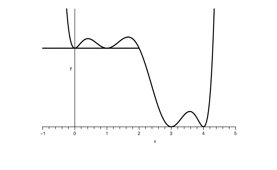
Figure 1 has a graph of QQ and χ(−∞,xℓ]\chi_{(-\infty,x_{\ell}]} for n=5n=5, ℓ=3\ell=3, xj=j−1x_{j}=j-1.

Refer to caption
Figure 1. An interpolation polynomial
Proof.

By standard interpolation theory, there exists a unique polynomial of degree kk with k+1k+1 conditions of the form

Q⁡(yj)=Q′​(yj)=⋯=Q(nj)​(yj)=0Q(y_{j})=Q^{\prime}(y_{j})=\cdots=Q^{(n_{j})}(y_{j})=0

∑jnj=k+1\sum_{j}n_{j}=k+1. Let QQ be the polynomial of degree 2​n−22n-2 with the nn conditions in (7.1) and the n−1n-1 conditions

Q′​(xj)=0j=1,…,ℓ−1,ℓ+1,…,nQ^{\prime}(x_{j})=0\qquad j=1,\dots,\ell-1,\ell+1,\dots,n (7.3)

Clearly, Q′Q^{\prime} has at most 2​n−32n-3 zeros. n−1n-1 are given by (7.3) and, by Snell’s theorem, each of the n−2n-2 intervals (x1,x2),…,(xℓ−1,xℓ),(xℓ+1,xℓ+2),…,(xn−1,xn)(x_{1},x_{2}),\dots,(x_{\ell-1},x_{\ell}),(x_{\ell+1},x_{\ell+2}),\dots,(x_{n-1},x_{n}) must have a zero. Since Q′Q^{\prime} is nonvanishing on (xℓ,xℓ+1)(x_{\ell},x_{\ell+1}) and Q⁡(xℓ)=1>Q⁡(xℓ+1)=0Q(x_{\ell})=1>Q(x_{\ell+1})=0, Q′​(y)<0Q^{\prime}(y)<0 on (xℓ,xℓ+1)(x_{\ell},x_{\ell+1}). Tracking where Q′Q^{\prime} changes sign, one sees that (7.2) holds. ∎

Theorem 7.2.

Suppose d​μd\mu is a measure on ℝ{\mathbb{R}} with finite moments. Then

∑{j∣xj(n)​(x0)≤x0}1Kn−1​(xj(n)​(x0),xj(n)​(x0))≥μ((−∞,x0])≥μ⁡((,,,))≥∑{j∣xj(n)​(x0)<x0}1Kn−1​(xj(n)​(x0),xj(n)​(x0))\begin{split}&\sum_{\{j\mid x_{j}^{(n)}(x_{0})\leq x_{0}\}}\frac{1}{K_{n-1}(x_{j}^{(n)}(x_{0}),x_{j}^{(n)}(x_{0}))}\geq\mu((-\infty,x_{0}])\\ &\qquad\geq\mu((-\infty,x_{0}))\geq\sum_{\{j\mid x_{j}^{(n)}(x_{0})<x_{0}\}}\frac{1}{K_{n-1}(x_{j}^{(n)}(x_{0}),x_{j}^{(n)}(x_{0}))}\end{split} (7.4)
Remarks.

1. The two bounds differ by Kn−1​(x0,x0)−1K_{n-1}(x_{0},x_{0})^{-1}.

2. These imply

μ⁡({x0})≤Kn−1​(x0,x0)−1\mu(\{x_{0}\})\leq K_{n-1}(x_{0},x_{0})^{-1} (7.5)

In fact, one knows (see (9.21) below)

μ⁡({x0})=limn→∞Kn−1​(x0,x0)−1\mu(\{x_{0}\})=\lim_{n\to\infty}\,K_{n-1}(x_{0},x_{0})^{-1} (7.6)

If μ⁡({x0})=0\mu(\{x_{0}\})=0, then the bounds are exact as n→∞n\to\infty.

Proof.

Suppose Pn−1​(x0)≠0P_{n-1}(x_{0})\neq 0. Let ℓ\ell be such that xℓ(n)​(x0)=x0x_{\ell}^{(n)}(x_{0})=x_{0}. Let QQ be the polynomial of Lemma 7.1. By (7.2),

μ((−∞,x0])≤∫Q(x)dμ\mu((-\infty,x_{0}])\leq\int Q(x)\,d\mu

and, by (7.1) and Theorem 6.5, the integral is the sum on the left of (7.4).

Clearly, this implies

μ⁡((x0,∞))≥∑{j∣xj(n)​(x0)>x0}1Kn−1​(xj(n)​(x0),xj(n)​(x0))\mu((x_{0},\infty))\geq\sum_{\{j\mid x_{j}^{(n)}(x_{0})>x_{0}\}}\frac{1}{K_{n-1}(x_{j}^{(n)}(x_{0}),x_{j}^{(n)}(x_{0}))}

which, by x→−xx\to-x symmetry, implies the last inequality in (7.4). ∎

Corollary 7.3.

If ℓ≤k−1\ell\leq k-1, then

∑j=ℓ+1k−11K⁡(xj(n)​(x0),xj(n)​(x0))\displaystyle\sum_{j=\ell+1}^{k-1}\frac{1}{K(x_{j}^{(n)}(x_{0}),x_{j}^{(n)}(x_{0}))} ≤μ⁡([xℓ(n)​(x0),xk(n)​(x0)])\displaystyle\leq\mu([x_{\ell}^{(n)}(x_{0}),x_{k}^{(n)}(x_{0})]) (7.7)
≤∑j=ℓk1K⁡(xj(n)​(x0),xj(n)​(x0))\displaystyle\leq\sum_{j=\ell}^{k}\frac{1}{K(x_{j}^{(n)}(x_{0}),x_{j}^{(n)}(x_{0}))}
Proof.

Note if x1=xℓ(n)​(x0)x_{1}=x_{\ell}^{(n)}(x_{0}) for some ℓ\ell, then xj(n)​(x0)=xj(n)​(x1)x_{j}^{(n)}(x_{0})=x_{j}^{(n)}(x_{1}), so we get (7.7) by subtracting values of (7.4). ∎

Notice that this corollary gives effective lower bounds only if k−1≥ℓ+1k-1\geq\ell+1, that is, only on at least three consecutive zeros. The following theorem of Last–Simon [58], based on ideas of Golinskii [42], can be used on successive zeros (see [58] for the proof).

Theorem 7.4.

If E,E′E,E^{\prime} are distinct zeros of Pn​(x)P_{n}(x), E~=12​(E+E′)\widetilde{E}=\frac{1}{2}(E+E^{\prime}) and δ>12​|E−E′|\delta>\frac{1}{2}\lvert E-E^{\prime}\rvert, then

|E−E′|≥δ2−(12​|E−E′|2)23​n​[Kn​(E,E)sup|y−E~|≤δKn​(y,y)]1/2\lvert E-E^{\prime}\rvert\geq\frac{\delta^{2}-(\frac{1}{2}\lvert E-E^{\prime}\rvert^{2})^{2}}{3n}\biggl[\frac{K_{n}(E,E)}{\sup_{\lvert y-\widetilde{E}\rvert\leq\delta}K_{n}(y,y)}\biggr]^{1/2} (7.8)

8. Mixed CD Kernels

Recall that given a measure μ\mu on ℝ{\mathbb{R}} with finite moments and Jacobi parameters {an,bn}n=1∞\{a_{n},b_{n}\}_{n=1}^{\infty}, the second kind polynomials are defined by the recursion relations (1.5) but with initial conditions

q0​(x)=0q1​(x)=a1−1q_{0}(x)=0\qquad q_{1}(x)=a_{1}^{-1} (8.1)

so qn​(x)q_{n}(x) is a polynomial of degree n−1n-1. In fact, if μ~\tilde{\mu} is the measure with Jacobi parameters given by

a~n=an+1b~n=bn+1\tilde{a}_{n}=a_{n+1}\qquad\tilde{b}_{n}=b_{n+1}

then

qn​(x,d​μ)=a1−1​pn−1​(x,d​μ~)q_{n}(x;d\mu)=a_{1}^{-1}p_{n-1}(x;d\tilde{\mu}) (8.2)

It is sometimes useful to consider

Kn(q)​(x,y)=∑j=0nqj​(x)¯​qj​(y)K_{n}^{(q)}(x,y)=\sum_{j=0}^{n}\,\overline{q_{j}(x)}\,q_{j}(y) (8.3)

and the mixed CD kernel

Kn(p​q)​(x,y)=∑j=0nqj​(x)¯​pj​(y)K_{n}^{(pq)}(x,y)=\sum_{j=0}^{n}\,\overline{q_{j}(x)}\,p_{j}(y) (8.4)

Since (8.2) implies

Kn(q)​(x,y,d​μ)=a1−2​Kn−1​(x,y,d​μ~)K_{n}^{(q)}(x,y;d\mu)=a_{1}^{-2}K_{n-1}(x,y;d\tilde{\mu}) (8.5)

there is a CD formula for K(q)K^{(q)} which follows immediately from the one for KK. There is also a mixed CD formula for Kn(p​q)K_{n}^{(pq)}.

OPUC also have second kind polynomials, mixed CD kernels, and mixed CD formulae. These are discussed in Section 3.2 of [81].

Mixed CD kernels will enter in Section 21.

9. Variational Principle: Basics

If one thing marks the OP approach to the CD kernel that has been missing from the spectral theorists’ approach, it is a remarkable variational principle for the diagonal kernel. We begin with:

Lemma 9.1.

Fix (α1,…,αm)∈ℂm(\alpha_{1},\dots,\alpha_{m})\in{\mathbb{C}}^{m}. Then

min⁡(∑j=1m|zj|2|∑j=1mαj​zj=1)=(∑j=1m|αj|2)−1\min\biggl(\,\sum_{j=1}^{m}\lvert z_{j}\rvert^{2}\biggm|\sum_{j=1}^{m}\alpha_{j}z_{j}=1\biggr)=\biggl(\,\sum_{j=1}^{m}\,\lvert\alpha_{j}\rvert^{2}\biggr)^{-1} (9.1)

with the minimizer given uniquely by

zj(0)=α¯j∑j=1m|αj|2z_{j}^{(0)}=\frac{\bar{\alpha}_{j}}{\sum_{j=1}^{m}\,\lvert\alpha_{j}\rvert^{2}} (9.2)
Remark.

One can use Lagrange multipliers to a priori compute zj(0)z_{j}^{(0)} and prove this result.

Proof.

If

∑j=1mαj​zj=1\sum_{j=1}^{m}\alpha_{j}z_{j}=1 (9.3)

then

∑j=1m|zj−zj(0)|2=∑j=1m|zj|2−(∑j=1m|αj|2)−1\sum_{j=1}^{m}\,\lvert z_{j}-z_{j}^{(0)}\rvert^{2}=\sum_{j=1}^{m}\,\lvert z_{j}\rvert^{2}-\biggl(\,\sum_{j=1}^{m}\,\lvert\alpha_{j}\rvert^{2}\biggr)^{-1} (9.4)

from which the result is obvious. ∎

If QQ has deg⁡(Q)≤n\deg(Q)\leq n and Qn​(z0)=1Q_{n}(z_{0})=1, then

Qn​(z)=∑j=0nαj​xj​(z)Q_{n}(z)=\sum_{j=0}^{n}\alpha_{j}x_{j}(z) (9.5)

with xjx_{j} the orthonormal polynomials for a measure d​μd\mu, then ∑αj​xj​(z0)=1\sum\alpha_{j}x_{j}(z_{0})=1 and ∥Qn∥L2​(ℂ,d​μ)2=∑j=0n|αj|2\lVert Q_{n}\rVert_{L^{2}({\mathbb{C}},d\mu)}^{2}=\sum_{j=0}^{n}\lvert\alpha_{j}\rvert^{2}. Thus the lemma implies:

Theorem 9.2 (Christoffel Variational Principle).

Let μ\mu be a measure on ℂ{\mathbb{C}} with finite moments. Then for z¯0∈ℂ\bar{z}_{0}\in{\mathbb{C}},

min⁡(∫|Qn​(z)|2​𝑑μ|Qn​(z0)=1,deg⁡(Qn)≤n)=1Kn​(z0,z0)\min\biggl(\int\lvert Q_{n}(z)\rvert^{2}\,d\mu\biggm|Q_{n}(z_{0})=1,\,\deg(Q_{n})\leq n\biggr)=\frac{1}{K_{n}(z_{0},z_{0})} (9.6)

and the minimizer is given by

Qn​(z,z0)=Kn​(z0,z)Kn​(z0,z0)Q_{n}(z,z_{0})=\frac{K_{n}(z_{0},z)}{K_{n}(z_{0},z_{0})} (9.7)

One immediate useful consequence is:

Theorem 9.3.

If μ≤ν\mu\leq\nu, then

Kn​(z,z,d​ν)≤Kn​(z,z,d​μ)K_{n}(z,z;d\nu)\leq K_{n}(z,z;d\mu) (9.8)

For this reason, it is useful to have comparison models:

Example 9.4.

Let d​μ=d​θ/2​πd\mu=d\theta/2\pi for z=r​ei​θz=re^{i\theta} and ζ=ei​φ\zeta=e^{i\varphi}. We have, since φn​(z)=zn\varphi_{n}(z)=z^{n},

Kn​(z,ζ)=1−rn+1​ei​(n+1)​(φ−θ)1−r​ei⁡(φ−θ)K_{n}(z,\zeta)=\frac{1-r^{n+1}e^{i(n+1)(\varphi-\theta)}}{1-re^{i(\varphi-\theta)}} (9.9)

If r<1r<1, Kn​(z,z0)K_{n}(z,z_{0}) has a limit as n→∞n\to\infty, and for z=ei​φz=e^{i\varphi}, z0=r​ei​θz_{0}=re^{i\theta}, r<1r<1,

|Qn​(z,z0)|2​d​φ2​π→Pr​(θ,φ)​d​φ2​π\lvert Q_{n}(z,z_{0})\rvert^{2}\,\frac{d\varphi}{2\pi}\to P_{r}(\theta,\varphi)\,\frac{d\varphi}{2\pi} (9.10)

the Poisson kernel,

Pr​(θ,φ)=1−r21+r2−2​r​cos⁡(θ−φ)P_{r}(\theta,\varphi)=\frac{1-r^{2}}{1+r^{2}-2r\cos(\theta-\varphi)} (9.11)

For r=1r=1, we have

|Kn​(ei​θ,ei​φ)|2=sin2⁡(n+12​(θ−φ))sin2⁡(θ−φ)\lvert K_{n}(e^{i\theta},e^{i\varphi})\rvert^{2}=\frac{\sin^{2}(\frac{n+1}{2}(\theta-\varphi))}{\sin^{2}(\theta-\varphi)} (9.12)

the Fejér kernel.

For r>1r>1, we use

Kn​(z,ζ)=z¯n​ζn​Kn​(1z,1ζ)K_{n}(z,\zeta)=\bar{z}^{n}\zeta^{n}K_{n}\biggl(\frac{1}{z}\,,\frac{1}{\zeta}\biggr) (9.13)

which implies, for z=ei​φz=e^{i\varphi}, z0=r​ei​θz_{0}=re^{i\theta}, r>1r>1,

|Qn​(z,z0)|2​d​φ2​π→Pr−1​(θ,φ)​d​φ2​π\lvert Q_{n}(z,z_{0})\rvert^{2}\,\frac{d\varphi}{2\pi}\to P_{r^{-1}}(\theta,\varphi)\,\frac{d\varphi}{2\pi} (9.14)

∎

Example 9.5.

Let d​μ0d\mu_{0} be the measure

d​μ0​(x)=12​π​4−x2​χ[−2,2]​(x)​d​xd\mu_{0}(x)=\frac{1}{2\pi}\,\sqrt{4-x^{2}}\,\chi_{[-2,2]}(x)\,dx (9.15)

on [−2,2][-2,2]. Then pnp_{n} are the Chebyshev polynomials of the second kind,

pn​(2​cos⁡θ)=sin⁡(n+1)​θsin⁡θp_{n}(2\cos\theta)=\frac{\sin(n+1)\theta}{\sin\theta} (9.16)

In particular, if |x|≤2−δ\lvert x\rvert\leq 2-\delta,

|pn​(x+i​y)|≤C1,δ​en​C2,δ​|y|\lvert p_{n}(x+iy)\rvert\leq C_{1,\delta}e^{nC_{2,\delta}\lvert y\rvert} (9.17)

and so

1n​|Kn​(x+i​y,x+i​y)|≤C1,δ2​e2​n​C2,δ​|y|\frac{1}{n}\,\lvert K_{n}(x+iy,x+iy)\rvert\leq C_{1,\delta}^{2}e^{2nC_{2,\delta}\lvert y\rvert} (9.18)

∎

The following shows the power of the variational principle:

Theorem 9.6.

Let

d​μ=w⁡(x)​d​x+d​μsd\mu=w(x)\,dx+d\mu_{\text{\rm{s}}} (9.19)

Suppose for some x0,δx_{0},\delta, we have

w⁡(x)≥c>0w(x)\geq c>0

for x∈[x0−δ,x0+δ]x\in[x_{0}-\delta,x_{0}+\delta]. Then for any δ′<δ\delta^{\prime}<\delta and all x∈[x0−δ′,x0+δ′]x\in[x_{0}-\delta^{\prime},x_{0}+\delta^{\prime}], we have for all aa real,

1n​Kn​(x+i​an,x+i​an)≤C1​eC2​|a|\frac{1}{n}\,K_{n}\biggl(x+\frac{ia}{n},x+\frac{ia}{n}\biggr)\leq C_{1}e^{C_{2}\lvert a\rvert} (9.20)
Proof.

We can find a scaled and translated version of the d​μ0d\mu_{0} of (9.15) with μ≥μ0\mu\geq\mu_{0}. Now use Theorem 9.3 and (9.18). ∎

The following has many proofs, but it is nice to have a variational one:

Theorem 9.7.

Let μ\mu be a measure on ℝ{\mathbb{R}} of compact support. For all x0∈ℝx_{0}\in{\mathbb{R}},

limn→∞Kn​(x0,x0)=μ​({x0})−1\lim_{n\to\infty}\,K_{n}(x_{0},x_{0})=\mu(\{x_{0}\})^{-1} (9.21)
Remark.

If μ⁡({x0})=0\mu(\{x_{0}\})=0, the limit is infinite.

Proof.

Clearly, if Q⁡(x0)=1Q(x_{0})=1, ∫|Qn​(x)|2​𝑑μ≥μ⁡({x0})\int\lvert Q_{n}(x)\rvert^{2}\,d\mu\geq\mu(\{x_{0}\}), so

Kn​(x0,x0)≤μ​({x0})−1K_{n}(x_{0},x_{0})\leq\mu(\{x_{0}\})^{-1} (9.22)

On the other hand, pick A≥diam⁡(σ⁡(d​μ))A\geq\diam(\sigma(d\mu)) and let

Q2​n​(x)=(1−(x−x0)2A2)nQ_{2n}(x)=\biggl(1-\frac{(x-x_{0})^{2}}{A^{2}}\biggr)^{n} (9.23)

For any aa,

sup|x−x0|≥ax∈σ⁡(d​μ)|Q2​n​(x)|≡M2​n​(a)→0\sup_{\begin{subarray}{c}\lvert x-x_{0}\rvert\geq a\\ x\in\sigma(d\mu)\end{subarray}}\lvert Q_{2n}(x)\rvert\equiv M_{2n}(a)\to 0 (9.24)

so, since Q2​n≤1Q_{2n}\leq 1 on σ⁡(d​μ)\sigma(d\mu),

Kn​(x0,x0)≥[μ⁡((,,,))+M2​n​(a)]−1K_{n}(x_{0},x_{0})\geq[\mu((x_{0}-a,x_{0}+a))+M_{2n}(a)]^{-1} (9.25)

so

lim infKn​(x0,x0)≥[μ⁡((,,,))]\liminf\,K_{n}(x_{0},x_{0})\geq[\mu((x_{0}-a,x_{0}+a))] (9.26)

for each aa. Since lima↓0μ⁡((,,,))=μ⁡({x0})\lim_{a\downarrow 0}\mu((x_{0}-a,x_{0}+a))=\mu(\{x_{0}\}), (9.22) and (9.26) imply (9.21). ∎

10. The Nevai Class: An Aside

In his monograph, Nevai [68] emphasized the extensive theory that can be developed for OPRL measures whose Jacobi parameters obey

an→abn→ba_{n}\to a\qquad b_{n}\to b (10.1)

for some bb real and a>0a>0. He proved such measures have ratio asymptotics, that is, Pn+1​(z)/Pn​(z)P_{n+1}(z)/P_{n}(z) has a limit for all z∈ℂ∖ℝz\in{\mathbb{C}}\setminus{\mathbb{R}}, and Simon [79] proved a converse: Ratio asymptotics at one point of ℂ+{\mathbb{C}}_{+} implies there are a,b,a,b, with (10.1). The essential spectrum for such a measure is [b−2​a,b+2​a][b-2a,b+2a], so the Nevai class is naturally associated with a single interval 𝔢⊂ℝ{\mathfrak{e}}\subset{\mathbb{R}}.

The question of what is the proper analog of the Nevai class for a set 𝔢{\mathfrak{e}} of the form

𝔢=[α1,β1]∪[α2,β2]∪…​[αℓ+1,βℓ+1]{\mathfrak{e}}=[\alpha_{1},\beta_{1}]\cup[\alpha_{2},\beta_{2}]\cup\dots[\alpha_{\ell+1},\beta_{\ell+1}] (10.2)

with

α1<β1<⋯<αℓ+1<βℓ+1\alpha_{1}<\beta_{1}<\cdots<\alpha_{\ell+1}<\beta_{\ell+1} (10.3)

has been answered recently and is relevant below.

The key was the realization of López [9, 10] that the proper analog of an arc of a circle was |αn|→a\lvert\alpha_{n}\rvert\to a and α¯n+1​αn→a2\bar{\alpha}_{n+1}\alpha_{n}\to a^{2} for some a>0a>0. This is not that αn\alpha_{n} approaches a fixed sequence but rather that for each kk,

min⁡∑j=nn+kei​θ∈∂𝔻⁡|αj−a​ei​θ|→0\min_{e^{i\theta}\in\partial{\mathbb{D}}}\,\sum_{j=n}^{n+k}\,\lvert\alpha_{j}-ae^{i\theta}\rvert\to 0 (10.4)

as n→∞n\to\infty. Thus, αj\alpha_{j} approaches a set of Verblunsky coefficients rather than a fixed one.

For any finite gap set 𝔢{\mathfrak{e}} of the form (10.2)/(10.3), there is a natural torus, 𝒥𝔢{\mathcal{J}}_{\mathfrak{e}}, of almost periodic Jacobi matrics with σess​(J)=𝔢\sigma_{\text{\rm{ess}}}(J)={\mathfrak{e}} for all J∈𝒥𝔢J\in{\mathcal{J}}_{\mathfrak{e}}. This can be described in terms of minimal Herglotz functions [91, 90] or reflectionless two-sided Jacobi matrices [76]. All J∈𝒥𝔢J\in{\mathcal{J}}_{\mathfrak{e}} are periodic if and only if each [αj,βj][\alpha_{j},\beta_{j}] has rational harmonic measure. In this case, we say 𝔢{\mathfrak{e}} is periodic.

Definition.
dm​({an,bn}n=1∞,{a~n,b~n}n=1∞)=∑j=0∞e−j​(|am+j−a~m+j|+|bm+j−b~m+j|)\displaystyle d_{m}(\{a_{n},b_{n}\}_{n=1}^{\infty},\{\tilde{a}_{n},\tilde{b}_{n}\}_{n=1}^{\infty})=\sum_{j=0}^{\infty}e^{-j}(\lvert a_{m+j}-\tilde{a}_{m+j}\rvert+\lvert b_{m+j}-\tilde{b}_{m+j}\rvert) (10.5)
dm​({an,bn},𝒥𝔢)=minJ∈𝒥𝔢⁡dm​({an,bn},J)\displaystyle d_{m}(\{a_{n},b_{n}\},{\mathcal{J}}_{\mathfrak{e}})=\min_{J\in{\mathcal{J}}_{\mathfrak{e}}}\,d_{m}(\{a_{n},b_{n}\},J) (10.6)
Definition.

The Nevai class for 𝔢{\mathfrak{e}}, N⁡(𝔢)N({\mathfrak{e}}), is the set of all Jacobi matrices, JJ, with

dm​(J,𝒥𝔢)→0d_{m}(J,{\mathcal{J}}_{\mathfrak{e}})\to 0 (10.7)

as m→∞m\to\infty.

This definition is implicit in Simon [82]; the metric dmd_{m} is from [27]. Notice that in case of a single gap 𝔢{\mathfrak{e}} in ∂𝔻\partial{\mathbb{D}}, the isospectral torus is the set of {αn}n=0∞\{\alpha_{n}\}_{n=0}^{\infty} with αn=a​ei​θ\alpha_{n}=ae^{i\theta} for all nn where aa is 𝔢{\mathfrak{e}} dependent and fixed and θ\theta is arbitrary. The above definition is the López class.

That this is the “right” definition is seen by the following pair of theorems:

Theorem 10.1 (Last–Simon [57]).

If J∈N⁡(𝔢)J\in N({\mathfrak{e}}), then

σess​(J)=𝔢\sigma_{\text{\rm{ess}}}(J)={\mathfrak{e}} (10.8)
Theorem 10.2 ([27] for periodic 𝔢{\mathfrak{e}}’s; [76] in general).

If

σess​(J)=σac​(J)=𝔢\sigma_{\text{\rm{ess}}}(J)=\sigma_{\text{\rm{ac}}}(J)={\mathfrak{e}}

then J∈N⁡(𝔢)J\in N({\mathfrak{e}}).

11. Delta Function Limits of Trial Polynomials

Intuitively, the minimizer, Qn​(x,x0)Q_{n}(x,x_{0}), in the Christoffel variational principle must be 11 at z0z_{0} and should try to be small on the rest of σ⁡(d​μ)\sigma(d\mu). As the degree gets larger and larger, one expects it can do this better and better. So one might guess that for every δ>0\delta>0,

sup|x−x0|>δx∈σ⁡(d​μ)|Qn​(x,x0)|→0\sup_{\begin{subarray}{c}\lvert x-x_{0}\rvert>\delta\\ x\in\sigma(d\mu)\end{subarray}}\lvert Q_{n}(x,x_{0})\rvert\to 0 (11.1)

While this happens in many cases, it is too much to hope for. If x1∈σ⁡(d​μ)x_{1}\in\sigma(d\mu) but μ\mu has very small weight near x1x_{1}, then it may be a better strategy for QnQ_{n} not to be small very near x1x_{1}. Indeed, we will see (Example 11.3) that the sup\sup in (11.1) can go to infinity. What is more likely is to expect that |Qn​(x,x0)|2​d​μ\lvert Q_{n}(x,x_{0})\rvert^{2}\,d\mu will be concentrated near x0x_{0}. We normalize this to define

d​ηn(x0)​(x)=|Qn​(x,x0)|2​d​μ​(x)∫|Qn​(x,x0)|2​𝑑μ​(x)d\eta_{n}^{(x_{0})}(x)=\frac{\lvert Q_{n}(x,x_{0})\rvert^{2}\,d\mu(x)}{\int\lvert Q_{n}(x,x_{0})\rvert^{2}\,d\mu(x)} (11.2)

so, by (9.6)/(9.7), in the OPRL case,

d​ηn(x0)​(x)=|Kn​(x,x0)|2Kn​(x,x0)​d​μ​(x)d\eta_{n}^{(x_{0})}(x)=\frac{\lvert K_{n}(x,x_{0})\rvert^{2}}{K_{n}(x,x_{0})}\,d\mu(x) (11.3)

We say μ\mu obeys the Nevai δ\delta-convergence criterion if and only if, in the sense of weak (aka vague) convergence of measures,

d​ηn(x0)​(x)→δx0d\eta_{n}^{(x_{0})}(x)\to\delta_{x_{0}} (11.4)

the point mass at x0x_{0}. In this section, we will explore when this holds.

Clearly, if x0∉σ⁡(d​μ)x_{0}\notin\sigma(d\mu), (11.4) cannot hold. We saw, for OPUC with d​μ=d​θ/2​πd\mu=d\theta/2\pi and z∉∂𝔻z\notin\partial{\mathbb{D}}, the limit was a Poisson measure, and similar results should hold for suitable OPRL. But we will see below (Example 11.2) that even on σ⁡(d​μ)\sigma(d\mu), (11.4) can fail. The major result below is that for Nevai class on 𝔢int{\mathfrak{e}}^{\text{\rm{int}}}, it does hold. We begin with an equivalent criterion:

Definition.

We say Nevai’s lemma holds if

limn→∞|pn​(x0)|2Kn​(x0,x0)=0\lim_{n\to\infty}\,\frac{\lvert p_{n}(x_{0})\rvert^{2}}{K_{n}(x_{0},x_{0})}=0 (11.5)
Theorem 11.1.

If d​μd\mu is a measure on ℝ{\mathbb{R}} with bounded support and

infnan>0\inf_{n}\,a_{n}>0 (11.6)

then for any fixed x0∈ℝx_{0}\in{\mathbb{R}},

(11.4)⇔(11.5)\eqref{11.4}\Leftrightarrow\eqref{11.5}
Remark.

That (11.5) ⇒\Rightarrow (11.4) is in Nevai [68]. The equivalence is a result of Breuer–Last–Simon [15].

Proof.

Since

1−Kn−1​(x0,x0)Kn​(x0,x0)=|pn​(x0)|2Kn​(x0,x0)\displaystyle 1-\frac{K_{n-1}(x_{0},x_{0})}{K_{n}(x_{0},x_{0})}=\frac{\lvert p_{n}(x_{0})\rvert^{2}}{K_{n}(x_{0},x_{0})} (11.7)
(11.5)⇔Kn−1​(x0,x0)Kn​(x0,x0)→1\displaystyle\eqref{11.5}\Leftrightarrow\frac{K_{n-1}(x_{0},x_{0})}{K_{n}(x_{0},x_{0})}\to 1 (11.8)

so

(11.5)⇒|pn+1​(x0)|2Kn​(x0,x0)=|pn+1​(x0)|2Kn+1​(x0,x0)​Kn+1​(x0,x0)Kn​(x0,x0)→0\eqref{11.5}\Rightarrow\frac{\lvert p_{n+1}(x_{0})\rvert^{2}}{K_{n}(x_{0},x_{0})}=\frac{\lvert p_{n+1}(x_{0})\rvert^{2}}{K_{n+1}(x_{0},x_{0})}\,\frac{K_{n+1}(x_{0},x_{0})}{K_{n}(x_{0},x_{0})}\to 0

We thus conclude

(11.5)⇔|pn​(x0)|2+|pn+1​(x0)|2Kn​(x0,x0)→0\eqref{11.5}\Leftrightarrow\frac{\lvert p_{n}(x_{0})\rvert^{2}+\lvert p_{n+1}(x_{0})\rvert^{2}}{K_{n}(x_{0},x_{0})}\to 0 (11.9)

By the CD formula and orthonormality of pj​(x)p_{j}(x),

∫|x−x0|2​|Kn​(x,x0)|2​𝑑μ=an+12​[pn​(x0)2+pn+1​(x0)2]\int\lvert x-x_{0}\rvert^{2}\lvert K_{n}(x,x_{0})\rvert^{2}\,d\mu=a_{n+1}^{2}[p_{n}(x_{0})^{2}+p_{n+1}(x_{0})^{2}] (11.10)

so, by (11.6) and (11.10),

∫|x−x0|2​d​ηn(x0)​(x)→0⇔(11.5)\int\lvert x-x_{0}\rvert^{2}\,d\eta_{n}^{(x_{0})}(x)\to 0\Leftrightarrow\eqref{11.5}

when ana_{n} is uniformly bounded above and away from zero. But since d​ηnd\eta_{n} have support in a fixed interval,

(11.4)⇔∫|x−x0|2​d​ηn(x0)→0∎\eqref{11.4}\Leftrightarrow\int\lvert x-x_{0}\rvert^{2}\,d\eta_{n}^{(x_{0})}\to 0\qed
Example 11.2.

Suppose at some point x0x_{0}, we have

limn→∞(|pn​(x0)|2+|pn+1​(x0)|2)1/n→A>1\lim_{n\to\infty}\,(\lvert p_{n}(x_{0})\rvert^{2}+\lvert p_{n+1}(x_{0})\rvert^{2})^{1/n}\to A>1 (11.11)

We claim that

lim supn→∞|pn​(x0)|2Kn​(x0,x0)>0\limsup_{n\to\infty}\,\frac{\lvert p_{n}(x_{0})\rvert^{2}}{K_{n}(x_{0},x_{0})}>0 (11.12)

for if (11.12) fails, then (11.5) holds and, by (11.7), for any ε\varepsilon, we can find N0N_{0} so for n≥N0n\geq N_{0},

Kn+1​(x0,x0)≤(1+ε)​Kn​(x0,x0)K_{n+1}(x_{0},x_{0})\leq(1+\varepsilon)K_{n}(x_{0},x_{0}) (11.13)

so

limKn​(x0,x0)1/n≤1\lim\,K_{n}(x_{0},x_{0})^{1/n}\leq 1

So, by (11.5), (11.11) fails. Thus, (11.11) implies that (11.5) fails, and so (11.4) fails. ∎

Remark.

As the proof shows, rather than a limit in (11.12), we can have a lim inf>1\liminf>1.

The first example of this type was found by Szwarc [95]. He has a d​μd\mu with pure points at 2−n−12-n^{-1} but not at 22, and so that the Lyapunov exponent at 22 was positive but 22 was not an eigenvalue, so (11.11) holds. The Anderson model (see [21]) provides a more dramatic example. The spectrum is an interval [a,b][a,b] and (11.11) holds for a.e. x∈[a,b]x\in[a,b]. The spectral measure in this case is supported at eigenvalues and at eigenvalues (11.8), and so (11.4) holds. Thus (11.4) holds on a dense set in [a,b][a,b] but fails for Lebesgue a.e. x0x_{0}!

Example 11.3.

A Jacobi weight has the form

d​μ​(x)=Ca,b​(1−x)a​(1+x)b​d​xd\mu(x)=C_{a,b}(1-x)^{a}(1+x)^{b}\,dx (11.14)

with a,b>−1a,b>-1. In general, one can show [94]

pn​(1)∼c​na+1/2p_{n}(1)\sim cn^{a+1/2} (11.15)

so if x0∈(−1,1)x_{0}\in(-1,1) where |pn​(x0)|2+|pn−1​(x0)|2\lvert p_{n}(x_{0})\rvert^{2}+\lvert p_{n-1}(x_{0})\rvert^{2} is bounded above and below, one has

|Kn​(x0,1)|Kn​(x0,x0)∼na+1/2n=na−1/2\frac{\lvert K_{n}(x_{0},1)\rvert}{K_{n}(x_{0},x_{0})}\sim\frac{n^{a+1/2}}{n}=n^{a-1/2}

so if a>12a>\frac{1}{2}, |Qn​(x0,1)|→∞\lvert Q_{n}(x_{0},1)\rvert\to\infty. Since d​μ​(x)d\mu(x) is small for xx near 11, one can (and, as we will see, does) have (11.4) even though (11.1) fails. ∎

With various counterexamples in place (and more later!), we turn to the positive results:

Theorem 11.4 (Nevai [68], Nevai–Totik–Zhang [70]).

If d​μd\mu is a measure in the classical Nevai class (i.e., for a single interval, 𝔢=[b−2​a,b+2​a]{\mathfrak{e}}=[b-2a,b+2a]), then (11.5) and so (11.4) holds uniformly on 𝔢{\mathfrak{e}}.

Theorem 11.5 (Zhang [109], Breuer–Last–Simon [15]).

Let 𝔢{\mathfrak{e}} be a periodic finite gap set and let μ\mu lie in the Nevai class for 𝔢{\mathfrak{e}}. Then (11.5) and so (11.4) holds uniformly on 𝔢{\mathfrak{e}}.

Theorem 11.6 (Breuer–Last–Simon [15]).

Let 𝔢{\mathfrak{e}} be a general finite gap set and let μ\mu lie in the Nevai class for 𝔢{\mathfrak{e}}. Then (11.5) and so (11.4) holds uniformly on compact subsets of 𝔢int{\mathfrak{e}}^{\text{\rm{int}}}.

Remarks.

1. Nevai [68] proved (10.4)/(10.5) for the classical Nevai class for every energy in 𝔢{\mathfrak{e}} but only uniformly on compacts of 𝔢int{\mathfrak{e}}^{\text{\rm{int}}}. Uniformity on all of 𝔢{\mathfrak{e}} using a beautiful lemma is from [70].

2. Zhang [109] proved Theorem 11.5 for any μ\mu whose Jacobi parameters approached a fixed periodic Jacobi matrix. Breuer–Last–Simon [15] noted that without change, Zhang’s result holds for the Nevai class.

3. It is hoped that the final version of [15] will prove the result in Theorem 11.6 on all of 𝔢{\mathfrak{e}}, maybe even uniformly in 𝔢{\mathfrak{e}}.

Example 11.7 ([15]).

In the next section, we will discuss regular measures. They have zero Lyapunov exponent on σess​(μ)\sigma_{\text{\rm{ess}}}(\mu), so one might expect Nevai’s lemma could hold—and it will in many regular cases. However, [15] prove that if bn≡0b_{n}\equiv 0 and ana_{n} is alternately 11 and 12\frac{1}{2} on successive very long blocks (11 on blocks of size 3n23^{n^{2}} and 12\frac{1}{2} on blocks of size 2n22^{n^{2}}), then d​μd\mu is regular for σ⁡(d​μ)=[−2,2]\sigma(d\mu)=[-2,2]. But for a.e. x∈[−2,2]∖[−1,1]x\in[-2,2]\setminus[-1,1], (10.4) and (10.3) fail. ∎

Conjecture 11.8 ([15]).

The following is extensively discussed in [15]: For general OPRL of compact support and a.e. xx with respect to μ\mu, (10.4) and so (10.3) holds.

12. Regularity: An Aside

There is another class besides the Nevai class that enters in variational problems because it allows exponential bounds on trial polynomials. It relies on notions from potential theory; see [43, 53, 74, 103] for the general theory and [92, 86] for the theory in the context of orthogonal polynomials.

Definition.

Let μ\mu be a measure with compact support and let 𝔢=σess​(μ){\mathfrak{e}}=\sigma_{\text{\rm{ess}}}(\mu). We say μ\mu is regular for 𝔢{\mathfrak{e}} if and only if

limn→∞(a1​…​an)1/n=C⁡(𝔢)\lim_{n\to\infty}\,(a_{1}\dots a_{n})^{1/n}=C({\mathfrak{e}}) (12.1)

the capacity of 𝔢{\mathfrak{e}}.

For 𝔢=[−1,1]{\mathfrak{e}}=[-1,1], C⁡(𝔢)=12C({\mathfrak{e}})=\frac{1}{2} and the class of regular measures was singled out initially by Erdős–Turán [33] and extensively studied by Ullman [104]. The general theory was developed by Stahl–Totik [92].

Recall that any set of positive capacity has an equilibrium measure, ρ𝔢\rho_{\mathfrak{e}}, and Green’s function, G𝔢G_{\mathfrak{e}}, defined by requiring G𝔢G_{\mathfrak{e}} is harmonic on ℂ∖𝔢{\mathbb{C}}\setminus{\mathfrak{e}}, G𝔢​(z)=log⁡|z|+O⁡(1)G_{\mathfrak{e}}(z)=\log\lvert z\rvert+O(1) near infinity, and for quasi-every x∈𝔢x\in{\mathfrak{e}},

limzn→xG𝔢​(zn)=0\lim_{z_{n}\to x}\,G_{\mathfrak{e}}(z_{n})=0 (12.2)

(quasi-every means except for a set of capacity 00). 𝔢{\mathfrak{e}} is called regular for the Dirichlet problem if and only if (12.2) holds for every x∈𝔢x\in{\mathfrak{e}}. Finite gap sets are regular for the Dirichlet problem.

One major reason regularity will concern us is:

Theorem 12.1.

Let 𝔢⊂ℝ{\mathfrak{e}}\subset{\mathbb{R}} be compact and regular for the Dirichlet problem. Let μ\mu be a measure regular for 𝔢{\mathfrak{e}}. Then for any ε\varepsilon, there is δ>0\delta>0 and CεC_{\varepsilon} so that

supdist​(z,𝔢)<δ|pn​(z,d​μ)|≤Cε​eε​|n|\sup_{\text{\rm{dist}}(z,{\mathfrak{e}})<\delta}\,\lvert p_{n}(z,d\mu)\rvert\leq C_{\varepsilon}e^{\varepsilon\lvert n\rvert} (12.3)

For proofs, see [92, 86]. Since KnK_{n} has n+1n+1 terms, (12.3) implies

supdist​(z,𝔢)<δdist​(w,𝔢)<δ|Kn​(z,w)|≤(n+1)​Cε2​e2​ε​|n|\sup_{\begin{subarray}{c}\text{\rm{dist}}(z,{\mathfrak{e}})<\delta\\ \text{\rm{dist}}(w,{\mathfrak{e}})<\delta\end{subarray}}\lvert K_{n}(z,w)\rvert\leq(n+1)C_{\varepsilon}^{2}e^{2\varepsilon\lvert n\rvert} (12.4)

and for the minimum (since Kn​(z0,z0)≥1K_{n}(z_{0},z_{0})\geq 1),

supdist​(z,𝔢)<δdist​(z0,𝔢)<δ|Qn​(z,z0)|≤(n+1)​Cε2​e2​ε​|n|\sup_{\begin{subarray}{c}\text{\rm{dist}}(z,{\mathfrak{e}})<\delta\\ \text{\rm{dist}}(z_{0},{\mathfrak{e}})<\delta\end{subarray}}\lvert Q_{n}(z,z_{0})\rvert\leq(n+1)C_{\varepsilon}^{2}e^{2\varepsilon\lvert n\rvert} (12.5)

The other reason regularity enters has to do with the density of zeros. If xj(n)x_{j}^{(n)} are the zeros of pn​(x,d​μ)p_{n}(x,d\mu), we define the zero counting measure, d​νnd\nu_{n}, to be the probability measure that gives weight to n−1n^{-1} to each xj(n)x_{j}^{(n)}. For the following, see [92, 86]:

Theorem 12.2.

Let 𝔢⊂ℝ{\mathfrak{e}}\subset{\mathbb{R}} be compact and let μ\mu be a regular measure for 𝔢{\mathfrak{e}}. Then

d​νn→d​ρ𝔢d\nu_{n}\to d\rho_{\mathfrak{e}} (12.6)

the equilibrium measure for 𝔢{\mathfrak{e}}.

In (12.6), the convergence is weak.

13. Weak Limits

A major theme in the remainder of this review is pointwise asymptotics of 1n+1​Kn​(x,y,d​μ)\frac{1}{n+1}K_{n}(x,y;d\mu) and its diagonal. Therefore, it is interesting that one can say something about 1n+1​Kn​(x,x,d​μ)​d​μ​(x)\frac{1}{n+1}K_{n}(x,x;d\mu)\,d\mu(x) without pointwise asymptotics. Notice that

d​μn​(x)≡1n+1​Kn​(x,x,d​μ)​d​μ​(x)d\mu_{n}(x)\equiv\frac{1}{n+1}\,K_{n}(x,x;d\mu)\,d\mu(x) (13.1)

is a probability measure. Recall the density of zeros, νn\nu_{n}, defined after (12.5).

Theorem 13.1.

Let μ\mu have compact support. Let νn\nu_{n} be the density of zeros and μn\mu_{n} given by (13.1). Then for any ℓ=0,1,2,…\ell=0,1,2,\dots,

|∫xℓ​d​νn+1−∫xℓ​d​μn|→0\biggl|\int x^{\ell}\,d\nu_{n+1}-\int x^{\ell}\,d\mu_{n}\biggr|\to 0 (13.2)

In particular, d​μn⁡(j)d\mu_{n(j)} and d​νn⁡(j)+1d\nu_{n(j)+1} have the same weak limits for any subsequence n⁡(j)n(j).

Proof.

By Theorem 6.2, the zeros of Pn+1P_{n+1} are eigenvalues of πn​Mx​πn\pi_{n}M_{x}\pi_{n}, so

∫xℓ​d​νn+1=1n+1​Tr​((πn​Mx​πn)ℓ)\int x^{\ell}\,d\nu_{n+1}=\frac{1}{n+1}\,\text{\rm{Tr}}((\pi_{n}M_{x}\pi_{n})^{\ell}) (13.3)

On the other hand, since {pj}j=0n\{p_{j}\}_{j=0}^{n} is a basis for ran​(πn)\text{\rm{ran}}(\pi_{n}),

∫xℓ​d​μn\displaystyle\int x^{\ell}\,d\mu_{n} =1n+1​∑j=0n∫xℓ​|pj​(x)|2​𝑑μ​(x)\displaystyle=\frac{1}{n+1}\sum_{j=0}^{n}\int x^{\ell}\lvert p_{j}(x)\rvert^{2}\,d\mu(x)
=1n+1​Tr​(πn​Mxℓ​πn)\displaystyle=\frac{1}{n+1}\,\text{\rm{Tr}}(\pi_{n}M_{x}^{\ell}\pi_{n}) (13.4)

It is easy to see that (πn​Mx​πn)ℓ−πn​Mxℓ​πn(\pi_{n}M_{x}\pi_{n})^{\ell}-\pi_{n}M_{x}^{\ell}\pi_{n} is rank at most ℓ\ell, so

LHS of (13.2)≤ℓn+1​∥Mx∥ℓ\text{LHS of \eqref{13.2}}\leq\frac{\ell}{n+1}\,\lVert M_{x}\rVert^{\ell}

goes to 00 as n→∞n\to\infty for ℓ\ell fixed. ∎

Remark.

This theorem is due to Simon [89] although the basic fact goes back to Avron–Simon [8].

See Simon [89] for an interesting application to comparison theorems for limits of density of states. We immediately have:

Corollary 13.2.

Suppose that

d​μ=w⁡(x)​d​x+d​μsd\mu=w(x)\,dx+d\mu_{\text{\rm{s}}} (13.5)

with d​μsd\mu_{\text{\rm{s}}} Lebesgue singular, and on some open interval I⊂𝔢=σess​(d​μ)I\subset{\mathfrak{e}}=\sigma_{\text{\rm{ess}}}(d\mu) we have d​νn→d​ν∞d\nu_{n}\to d\nu_{\infty} and

d​ν∞↾I=ν∞​(x)​d​xd\nu_{\infty}\restriction I=\nu_{\infty}(x)\,dx (13.6)

and suppose that uniformly on II,

lim1n​Kn​(x,x)=g⁡(x)\lim\,\frac{1}{n}K_{n}(x,x)=g(x) (13.7)

and w⁡(x)≠0w(x)\neq 0 on II. Then

g⁡(x)=ν∞​(x)w⁡(x)g(x)=\frac{\nu_{\infty}(x)}{w(x)}
Proof.

The theorem implies d​ν∞↾I=w⁡(x)​g​(x)d\nu_{\infty}\restriction I=w(x)g(x). ∎

Thus, in the regular case, we expect that “usually”

1n​Kn​(x,x)→ρ𝔢​(x)w⁡(x)\frac{1}{n}\,K_{n}(x,x)\to\frac{\rho_{\mathfrak{e}}(x)}{w(x)} (13.8)

This is what we explore in much of the rest of this paper.

14. Variational Principle: Máté–Nevai Upper Bounds

The Cotes numbers, λn​(z0)\lambda_{n}(z_{0}), are given by (9.6), so upper bounds on λn​(z0)\lambda_{n}(z_{0}) mean lower bounds on diagonal CD kernels and there is a confusion of “upper bounds” and “lower bounds.” We will present here some very general estimates that come from the use of trial functions in (9.6) so they are called Máté–Nevai upper bounds (after [66]), although we will write them as lower bounds on KnK_{n}. One advantage is their great generality.

Definition.

Let d​μd\mu be a measure on ℝ{\mathbb{R}} of the form

d​μ=w⁡(x)​d​x+d​μsd\mu=w(x)\,dx+d\mu_{\text{\rm{s}}} (14.1)

where d​μsd\mu_{\text{\rm{s}}} is singular with respect to Lebesgue measure. We call x0x_{0} a Lebesgue point of μ\mu if and only if

n2​μs​([x0−1n,x0+1n])→0\displaystyle\frac{n}{2}\,\mu_{\text{\rm{s}}}\biggl(\biggl[x_{0}-\frac{1}{n},x_{0}+\frac{1}{n}\biggr]\biggr)\to 0 (14.2)
n2​∫x0−1nx0+1n|w⁡(x)−w0​(x0)|​𝑑x→0\displaystyle\frac{n}{2}\int_{x_{0}-\frac{1}{n}}^{x_{0}+\frac{1}{n}}\lvert w(x)-w_{0}(x_{0})\rvert\,dx\to 0 (14.3)

It is a fundamental fact of harmonic analysis ([77]) that for any μ\mu Lebesgue-a.e., x0x_{0} in ℝ{\mathbb{R}} is a Lebesgue point for μ\mu. Here is the most general version of the MN upper bound:

Theorem 14.1.

Let 𝔢⊂ℝ{\mathfrak{e}}\subset{\mathbb{R}} be an arbitrary compact set which is regular for the Dirichlet problem. Let I⊂𝔢I\subset{\mathfrak{e}} be a closed interval. Let d​μd\mu be a measure with compact support in ℝ{\mathbb{R}} with σess​(d​μ)⊂𝔢\sigma_{\text{\rm{ess}}}(d\mu)\subset{\mathfrak{e}}. Then for any Lebesgue point, xx in II,

lim infn→∞1n​Kn​(x,x)≥ρ𝔢​(x)w⁡(x)\liminf_{n\to\infty}\frac{1}{n}\,K_{n}(x,x)\geq\frac{\rho_{\mathfrak{e}}(x)}{w(x)} (14.4)

where d​ρ𝔢↾I=ρ𝔢​(x)​d​xd\rho_{\mathfrak{e}}\restriction I=\rho_{\mathfrak{e}}(x)\,dx. If ww is continuous on II (including at the endpoints as a function in a neighborhood of II) and nonvanishing, then (14.4) holds uniformly on II. If xn→x∈Ix_{n}\to x\in I and A=supnn​|xn−x|<∞A=\sup_{n}n\lvert x_{n}-x\rvert<\infty and xx is a Lebesgue, then (14.4) holds with Kn​(x,x)K_{n}(x,x) replaced by Kn​(xn,xn)K_{n}(x_{n},x_{n}). If ww is continuous and nonvanishing on II, then this extended convergence is uniform in x∈Ix\in I and xnx_{n}’s with A≤A0<∞A\leq A_{0}<\infty.

Remarks.

1. If I⊂𝔢I\subset{\mathfrak{e}} is a nontrivial interval, the measure d​ρ𝔢↾Id\rho_{\mathfrak{e}}\restriction I is purely absolutely continuous (see, e.g., [86, 90]).

2. For OPUC, this is a result of Máté–Nevai [65]. The translation to OPRL on [−1,1][-1,1] is explicit in Máté–Nevai–Totik [67]. The extension to general sets via polynomial mapping and approximation (see Section 18) is due to Totik [97]. These papers also require a local Szegő condition, but that is only needed for lower bounds on λn\lambda_{n} (see Section 17). They also don’t state the xn→x∞x_{n}\to x_{\infty} result, which is a refinement introduced by Lubinsky [61] who implemented it in certain [−1,1][-1,1] cases.

3. An alternate approach for Totik’s polynomial mapping is to use trial functions based on Jost–Floquet solutions for periodic problems; see Section 19 (and also [88, 90]).

One can combine (14.4) with weak convergence and regularity to get

Theorem 14.2 (Simon [89]).

Let 𝔢⊂ℝ{\mathfrak{e}}\subset{\mathbb{R}} be an arbitrary compact set, regular for the Dirichlet problem. Let d​μd\mu be a measure with compact support in ℝ{\mathbb{R}} with σess​(d​μ)=𝔢\sigma_{\text{\rm{ess}}}(d\mu)={\mathfrak{e}} and with d​μd\mu regular for 𝔢{\mathfrak{e}}. Let I⊂𝔢I\subset{\mathfrak{e}} be an interval so w⁡(x)>0w(x)>0 a.e. on II. Then

(i) ∫I|1n​Kn​(x,x)​w​(x)−ρ𝔢​(x)|​𝑑x→0\displaystyle\int_{I}\biggl|\frac{1}{n}\,K_{n}(x,x)\,w(x)-\rho_{\mathfrak{e}}(x)\biggr|dx\to 0 (14.5)
(ii) ∫I1n​Kn​(x,x)​d​μs​(x)→0\displaystyle\int_{I}\frac{1}{n}\,K_{n}(x,x)\,d\mu_{\text{\rm{s}}}(x)\to 0 (14.6)
Proof.

By Theorems 12.2 and 13.1,

1n​Kn​(x,x)​d​μ→d​ρ𝔢\frac{1}{n}\,K_{n}(x,x)\,d\mu\to d\rho_{\mathfrak{e}} (14.7)

Let ν1\nu_{1} be a limit point of 1n​Kn​(x,x)​d​μs\frac{1}{n}K_{n}(x,x)\,d\mu_{\text{\rm{s}}} and

d​ν2=d​ρ𝔢−d​ν1d\nu_{2}=d\rho_{\mathfrak{e}}-d\nu_{1} (14.8)

If f≥0f\geq 0, by Fatou’s lemma and (14.4),

∫If​d​ν2≥∫Iρ𝔢​(x)​f​(x)​𝑑x\int_{I}f\,d\nu_{2}\geq\int_{I}\rho_{\mathfrak{e}}(x)f(x)\,dx (14.9)

that is, d​ν2↾I≥ρ𝔢​(x)​d​x↾Id\nu_{2}\restriction I\geq\rho_{\mathfrak{e}}(x)\,dx\restriction I. By (14.8), d​ν2↾I≤ρ𝔢​(x)​d​xd\nu_{2}\restriction I\leq\rho_{\mathfrak{e}}(x)\,dx. It follows d​ν1↾Id\nu_{1}\restriction I is 00 and d​ν2↾I=d​ρ𝔢↾Id\nu_{2}\restriction I=d\rho_{\mathfrak{e}}\restriction I.

By compactness, 1n​Kn​(x,x)​d​μs↾I→0\frac{1}{n}K_{n}(x,x)\,d\mu_{\text{\rm{s}}}\restriction I\to 0 weakly, implying (14.6). By a simple argument [89], weak convergence of 1n​Kn​(x,x)​w​(x)​d​x→ρ𝔢​(x)​d​x\frac{1}{n}K_{n}(x,x)w(x)\,dx\to\rho_{\mathfrak{e}}(x)\,dx and (14.4) imply (14.5). ∎

15. Criteria for A.C. Spectrum

Define

N={x∈ℝ|lim inf1n​Kn​(x,x)<∞}N=\biggl\{x\in{\mathbb{R}}\biggm|\liminf\,\frac{1}{n}\,K_{n}(x,x)<\infty\biggr\} (15.1)

so that

ℝ∖N={x∈ℝ|lim1n​Kn​(x,x)=∞}{\mathbb{R}}\setminus N=\biggl\{x\in{\mathbb{R}}\biggm|\lim\,\frac{1}{n}\,K_{n}(x,x)=\infty\biggr\} (15.2)

Theorem 14.1 implies

Theorem 15.1.

Let 𝔢⊂ℝ{\mathfrak{e}}\subset{\mathbb{R}} be an arbitrary compact set and d​μ=w⁡(x)​d​x+d​μsd\mu=w(x)\,dx+d\mu_{\text{\rm{s}}} a measure with σ⁡(μ)=𝔢\sigma(\mu)={\mathfrak{e}}. Let Σac={x∣w⁡(x)>0}\Sigma_{\text{\rm{ac}}}=\{x\mid w(x)>0\}. Then N∖ΣacN\setminus\Sigma_{\text{\rm{ac}}} has Lebesgue measure zero.

Proof.

If x0∈ℝ∖Σacx_{0}\in{\mathbb{R}}\setminus\Sigma_{\text{\rm{ac}}} and is a Lebesgue point of μ\mu, then w⁡(x0)=0w(x_{0})=0 and, by Theorem 14.1, x0∈ℝ∖Nx_{0}\in{\mathbb{R}}\setminus N. Thus,

(ℝ∖Σac)∖(ℝ∖N)=N∖Σac({\mathbb{R}}\setminus\Sigma_{\text{\rm{ac}}})\setminus({\mathbb{R}}\setminus N)=N\setminus\Sigma_{\text{\rm{ac}}}

has Lebesgue measure zero. ∎

Remark.

This is a direct but not explicit consequence of the Máté–Nevai ideas [65]. Without knowing of this work, Theorem 15.1 was rediscovered with a very different proof by Last–Simon [56].

On the other hand, following Last–Simon [56], we note that Fatou’s lemma and

∫1n​Kn​(x,x)​𝑑μ​(x)=1\int\frac{1}{n}\,K_{n}(x,x)\,d\mu(x)=1 (15.3)

implies

∫lim inf⁡1n​Kn​(x,x)​𝑑μ​(x)≤1\int\liminf\,\frac{1}{n}\,K_{n}(x,x)\,d\mu(x)\leq 1 (15.4)

so

Theorem 15.2 ([56]).

Σac∖N\Sigma_{\text{\rm{ac}}}\setminus N has Lebesgue measure zero.

Thus, up to sets of measure zero, Σac=N\Sigma_{\text{\rm{ac}}}=N. What is interesting is that this holds, for example, when 𝔢{\mathfrak{e}} is a positive measure Cantor set as occurs for the almost Mathieu operator (an≡1CLOSE(a_{n}\equiv 1, bn=λ​cos⁡(π​α​n+θ)b_{n}=\lambda\cos(\pi\alpha n+\theta), |λ|<2\lvert\lambda\rvert<2, λ≠0\lambda\neq 0, α\alpha irrational). This operator has been heavily studied; see Last [55].

16. Variational Principle: Nevai Trial Polynomial

A basic idea is that if d​μ1d\mu_{1} and d​μ2d\mu_{2} look alike near x0x_{0}, there is a good chance that Kn​(x0,x0,d​μ1)K_{n}(x_{0},x_{0};d\mu_{1}) and Kn​(x0,x0,d​μ2)K_{n}(x_{0},x_{0};d\mu_{2}) are similar for nn large. The expectation (13.8) says they better have the same support (and be regular for that support), but this is a reasonable guess.

It is natural to try trial polynomials minimizing λn​(x0,d​μ1)\lambda_{n}(x_{0},d\mu_{1}) in the Christoffel variational principle for λn​(x0,d​μ2)\lambda_{n}(x_{0},d\mu_{2}), but Example 11.3 shows this will not work in general. If d​μ1d\mu_{1} has a strong zero near some other x1x_{1}, the trial polynomial for d​μ1d\mu_{1} may be large near x1x_{1} and be problematical for d​μ2d\mu_{2} if it does not have a zero there. Nevai [68] had the idea of using a localizing factor to overcome this.

Suppose 𝔢⊂ℝ{\mathfrak{e}}\subset{\mathbb{R}}, a compact set which, for now, we suppose contains σ⁡(d​μ1)\sigma(d\mu_{1}) and σ⁡(d​μ2)\sigma(d\mu_{2}). Pick A=diam⁡(𝔢)A=\diam({\mathfrak{e}}) and consider (with [⋅]≡[\,\cdot\,]\equiv integral part)

(1−(x−x0)2A2)[ε​n]≡N2​[ε​n]​(x)\biggl(1-\frac{(x-x_{0})^{2}}{A^{2}}\biggr)^{[\varepsilon n]}\equiv N_{2[\varepsilon n]}(x) (16.1)

Then for any δ\delta,

sup|x−x0|>δx∈𝔢N2​[ε​n]​(x)≤e−c⁡(δ,ε)​n\sup_{\begin{subarray}{c}\lvert x-x_{0}\rvert>\delta\\ x\in{\mathfrak{e}}\end{subarray}}N_{2[\varepsilon n]}(x)\leq e^{-c(\delta,\varepsilon)n} (16.2)

so if Qn−2​[ε​n]​(x)Q_{n-2[\varepsilon n]}(x) is the minimizer for μ1\mu_{1} and 𝔢{\mathfrak{e}} is regular for the Dirichlet problem and μ1\mu_{1} is regular for 𝔢{\mathfrak{e}}, then the Nevai trial function

N2​[ε​n]​(x)​Qn−2​[ε​n]​(x)N_{2[\varepsilon n]}(x)Q_{n-2[\varepsilon n]}(x)

will be exponentially small away from x0x_{0}.

For this to work to compare λn​(x0,d​μ1)\lambda_{n}(x_{0},d\mu_{1}) and λ⁡(x0,d​μ2)\lambda(x_{0},d\mu_{2}), we need two additional properties of λn​(x0,d​μ1)\lambda_{n}(x_{0},d\mu_{1}):

  • (a)

    λn​(x0,d​μ1)≥Cε​e−ε​n\lambda_{n}(x_{0},d\mu_{1})\geq C_{\varepsilon}e^{-\varepsilon n} for each ε<0\varepsilon<0. This is needed for the exponential contributions away from x0x_{0} not to matter.

  • (b)
    limε↓0lim supn→∞λn​(x0,d​μ1)λn−2​[ε​n]​(x,d​μ1)=1\lim_{\varepsilon\downarrow 0}\,\limsup_{n\to\infty}\,\frac{\lambda_{n}(x_{0},d\mu_{1})}{\lambda_{n-2[\varepsilon n]}(x,d\mu_{1})}=1

    so that the change from QnQ_{n} to Qn−2​[ε​n]Q_{n-2[\varepsilon n]} does not matter.

Notice that both (a) and (b) hold if

limn→∞n​λn​(x0,d​μ)=c>0\lim_{n\to\infty}\,n\lambda_{n}(x_{0},d\mu)=c>0 (16.3)

If one only has 𝔢=σess​(d​μ2){\mathfrak{e}}=\sigma_{\text{\rm{ess}}}(d\mu_{2}), one can use explicit zeros in the trial polynomials to mask the eigenvalues outside 𝔢{\mathfrak{e}}.

For details of using Nevai trial functions, see [88, 90]. Below we will just refer to using Nevai trial functions.

17. Variational Principle: Máté–Nevai–Totik Lower Bound

In [67], Máté–Nevai–Totik proved:

Theorem 17.1.

Let d​μd\mu be a measure on ∂𝔻\partial{\mathbb{D}}

d​μ=w⁡(θ)2​π​d​θ+d​μsd\mu=\frac{w(\theta)}{2\pi}\,d\theta+d\mu_{\text{\rm{s}}} (17.1)

which obeys the Szegő condition

∫log⁡(w⁡(θ))​d​θ2​π>−∞\int\log(w(\theta))\,\frac{d\theta}{2\pi}>-\infty (17.2)

Then for a.e. θ∞∈∂𝔻\theta_{\infty}\in\partial{\mathbb{D}},

lim infn​λn​(θ∞)≥w⁡(θ∞)\liminf\,n\lambda_{n}(\theta_{\infty})\geq w(\theta_{\infty}) (17.3)

This remains true if λn​(θ∞)\lambda_{n}(\theta_{\infty}) is replaced by λn​(θn)\lambda_{n}(\theta_{n}) with θn→θ∞\theta_{n}\to\theta_{\infty} obeying supn​|θn−θ∞|<∞\sup n\lvert\theta_{n}-\theta_{\infty}\rvert<\infty.

Remarks.

1. The proof in [67] is clever but involved ([90] has an exposition); it would be good to find a simpler proof.

2. [67] only has the result θn=θ∞\theta_{n}=\theta_{\infty}. The general θn\theta_{n} result is due to Findley [34].

3. The θ∞\theta_{\infty} for which this is proven have to be Lebesgue points for d​μd\mu as well as Lebesgue points for log⁡(w)\log(w) and for its conjugate function.

4. As usual, if II is an interval with ww continuous and nonvanishing, and μs​(I)=0\mu_{\text{\rm{s}}}(I)=0, (17.3) holds uniformly if θ∞∈I\theta_{\infty}\in I.

By combining this lower bound with the Máté–Nevai upper bound, we get the result of Máté–Nevai–Totik [67]:

Theorem 17.2.

Under the hypothesis of Theorem 17.1, for a.e. θ∞∈∂𝔻\theta_{\infty}\in\partial{\mathbb{D}},

limn→∞n​λn​(θ∞)=w⁡(θ∞)\lim_{n\to\infty}\,n\lambda_{n}(\theta_{\infty})=w(\theta_{\infty}) (17.4)

This remains true if λn​(θ∞)\lambda_{n}(\theta_{\infty}) is replaced by λn​(θn)\lambda_{n}(\theta_{n}) with θn→θ∞\theta_{n}\to\theta_{\infty} obeying supn​|θn−θ∞|<∞\sup n\lvert\theta_{n}-\theta_{\infty}\rvert<\infty. If II is an interval with ww continuous on II and μs​(I)=0\mu_{\text{\rm{s}}}(I)=0, then these results hold uniformly in II.

Remark.

It is possible (see remarks in Section 4.6 of [69]) that (17.4) holds if a Szegő condition is replaced by w⁡(θ)>0w(\theta)>0 for a.e. θ\theta. Indeed, under that hypothesis, Simon [89] proved that

∫02​π|w⁡(θ)​(n​λn​(θ))−1−1|​d​θ2​π→0\int_{0}^{2\pi}\lvert w(\theta)(n\lambda_{n}(\theta))^{-1}-1\rvert\,\frac{d\theta}{2\pi}\to 0

There have been significant extensions of Theorem 17.2 to OPRL on fairly general sets:

  • 1.

    [67] used the idea of Nevai trial functions (Section 16) to prove the Szegő condition could be replaced by regularity plus a local Szegő condition.

  • 2.

    [67] used the Szegő mapping to get a result for [−1,1][-1,1].

  • 3.

    Using polynomial mappings (see Section 18) plus approximation, Totik [97] proved a general result (see below); one can replace polynomial mappings by Floquet–Jost solutions (see Section 19) in the case of continuous weights on an interval (see [88]).

Here is Totik’s general result (extended from σ⁡(d​μ)⊂𝔢\sigma(d\mu)\subset{\mathfrak{e}} to σess​(d​μ)⊂𝔢\sigma_{\text{\rm{ess}}}(d\mu)\subset{\mathfrak{e}}):

Theorem 17.3 (Totik [97, 100]).

Let 𝔢{\mathfrak{e}} be a compact subset of ℝ{\mathbb{R}}. Let I⊂𝔢I\subset{\mathfrak{e}} be an interval. Let d​μd\mu have σess​(d​μ)=𝔢\sigma_{\text{\rm{ess}}}(d\mu)={\mathfrak{e}} be regular for 𝔢{\mathfrak{e}} with

∫Ilog⁡(w)​𝑑x>−∞\int_{I}\log(w)\,dx>-\infty (17.5)

Then for a.e. x∞∈Ix_{\infty}\in I,

limn→∞1n​Kn​(x∞,x∞)=ρ𝔢​(x∞)w⁡(x∞)\lim_{n\to\infty}\,\frac{1}{n}\,K_{n}(x_{\infty},x_{\infty})=\frac{\rho_{\mathfrak{e}}(x_{\infty})}{w(x_{\infty})} (17.6)

The same limit holds for 1n​Kn​(xn,xn)\frac{1}{n}K_{n}(x_{n},x_{n}) if supnn​|xn−x∞|<∞\sup_{n}n\lvert x_{n}-x_{\infty}\rvert<\infty. If μs​(I)=∅\mu_{\text{\rm{s}}}(I)=\emptyset and ww is continuous and nonvanishing on II, then those limits are uniform on x∞∈Ix_{\infty}\in I and on all xnx_{n}’s with supnn​|xn−x∞|≤A\sup_{n}n\lvert x_{n}-x_{\infty}\rvert\leq A (uniform for each fixed AA).

Remarks.

1. Totik [99] recently proved asymptotic results for suitable CD kernels for OPs which are neither OPUC nor OPRL.

2. The extension to general compact 𝔢{\mathfrak{e}} without an assumption of regularity for the Dirichlet problem is in [100].

18. Variational Principle: Polynomial Maps

In passing from [−1,1][-1,1] to fairly general sets, one uses a three-step process. A finite gap set is an 𝔢{\mathfrak{e}} of the form

𝔢=[α1,β1]∪[α2,β2]∪⋯∪[αℓ+1,βℓ+1]{\mathfrak{e}}=[\alpha_{1},\beta_{1}]\cup[\alpha_{2},\beta_{2}]\cup\cdots\cup[\alpha_{\ell+1},\beta_{\ell+1}] (18.1)

where

α1<β1<α2<β2<⋯<αℓ+1<βℓ+1\alpha_{1}<\beta_{1}<\alpha_{2}<\beta_{2}<\cdots<\alpha_{\ell+1}<\beta_{\ell+1} (18.2)

ℰf{\mathcal{E}}_{f} will denote the family of finite gap sets. We write 𝔢=𝔢1∪⋯∪𝔢ℓ+1{\mathfrak{e}}={\mathfrak{e}}_{1}\cup\cdots\cup{\mathfrak{e}}_{\ell+1} in this case with the 𝔢j{\mathfrak{e}}_{j} closed disjoint intervals. ℰp{\mathcal{E}}_{p} will denote the set of what we called periodic finite gap sets in Section 10—ones where each 𝔢j{\mathfrak{e}}_{j} has rational harmonic measure. Here are the three steps:

  • (1)

    Extend to 𝔢∈ℰp{\mathfrak{e}}\in{\mathcal{E}}_{p} using the methods discussed briefly below.

  • (2)

    Prove that given any 𝔢∈ℰf{\mathfrak{e}}\in{\mathcal{E}}_{f}, there is 𝔢(n)∈ℰp{\mathfrak{e}}^{(n)}\in{\mathcal{E}}_{p}, each with the same number of bands so 𝔢j⊂𝔢j(n)⊂𝔢j(n−1){\mathfrak{e}}_{j}\subset{\mathfrak{e}}_{j}^{(n)}\subset{\mathfrak{e}}_{j}^{(n-1)} and ∩n𝔢j(n)=𝔢j\cap_{n}{\mathfrak{e}}_{j}^{(n)}={\mathfrak{e}}_{j}. This is a result proven independently by Bogatyrëv [13], Peherstorfer [72], and Totik [98]; see [90] for a presentation of Totik’s method.

  • (3)

    Note that for any compact 𝔢{\mathfrak{e}}, if 𝔢(m)={x∣dist​(x,𝔢)≤1m}{\mathfrak{e}}^{(m)}=\{x\mid\text{\rm{dist}}(x,{\mathfrak{e}})\leq\frac{1}{m}\}, then 𝔢(m){\mathfrak{e}}^{(m)} is a finite gap set and 𝔢=∩m𝔢(m){\mathfrak{e}}=\cap_{m}{\mathfrak{e}}^{(m)}.

Step (1) is the subtle step in extending theorems: Given the Bogatyrëv–Peherstorfer–Totik theorem, the extensions are simple approximation.

The key to 𝔢∈ℰp{\mathfrak{e}}\in{\mathcal{E}}_{p} is that there is a polynomial Δ~:ℂ→ℂ\tilde{\Delta}\colon{\mathbb{C}}\to{\mathbb{C}}, so Δ~−1​([−1,1])=𝔢\tilde{\Delta}^{-1}([-1,1])={\mathfrak{e}} and so that 𝔢j{\mathfrak{e}}_{j} is a finite union of intervals 𝔢~k\tilde{\mathfrak{e}}_{k} with disjoint interiors so that Δ~\tilde{\Delta} is a bijection from each 𝔢~k\tilde{\mathfrak{e}}_{k} to [−1,1][-1,1]. That this could be useful was noted initially by Geronimo–Van Assche [37]. Totik showed how to prove Theorem 17.3 for 𝔢∈ℰp{\mathfrak{e}}\in{\mathcal{E}}_{p} from the results for [−1,1][-1,1] using this polynomial mapping.

For spectral theorists, the polynomial Δ~=12​Δ\tilde{\Delta}=\frac{1}{2}\Delta where Δ\Delta is the discriminant for the associated periodic problem (see [44, 54, 105, 96, 90]). There is a direct construction of Δ~\tilde{\Delta} by Aptekarev [5] and Peherstorfer [71, 72, 73].

19. Floquet–Jost Solutions for Periodic Jacobi Matrices

As we saw in Section 16, models with appropriate behavior are useful input for comparison theorems. Periodic Jacobi matrices have OPs for which one can study the CD kernel and its asymptotics. The two main results concern diagonal and just off-diagonal behavior:

Theorem 19.1.

Let μ\mu be the spectral measure associated to a periodic Jacobi matrix with essential spectrum, 𝔢{\mathfrak{e}}, a finite gap set. Let d​μ=w⁡(x)​d​xd\mu=w(x)\,dx on 𝔢{\mathfrak{e}} (there can also be up to one eigenvalue in each gap). Then uniformly for xx in compact subsets of 𝔢int{\mathfrak{e}}^{\text{\rm{int}}},

1n​Kn​(x,x)→ρ𝔢​(x)w⁡(x)\frac{1}{n}\,K_{n}(x,x)\to\frac{\rho_{\mathfrak{e}}(x)}{w(x)} (19.1)

and uniformly for such xx and a,ba,b in ℝ{\mathbb{R}} with |a|≤A\lvert a\rvert\leq A, |b|≤B\lvert b\rvert\leq B,

Kn​(x+an,x+bn)Kn​(x,x)→sin⁡(π​ρ𝔢​(x)​(b−a))π​ρ𝔢​(x)​(b−a)\frac{K_{n}(x+\frac{a}{n},x+\frac{b}{n})}{K_{n}(x,x)}\to\frac{\sin(\pi\rho_{\mathfrak{e}}(x)(b-a))}{\pi\rho_{\mathfrak{e}}(x)(b-a)} (19.2)
Remarks.

1. (19.2) is often called bulk universality. On bounded intervals, it goes back to random matrix theory. The best results using Riemann–Hilbert methods for OPs is due to Kuijlaars–Vanlessen [52]. A different behavior is expected at the edge of the spectrum—we will not discuss this in detail, but see Lubinsky [63].

2. For [−1,1][-1,1], Lubinsky [61] used Legendre polynomials as his model. The references for the proofs here are Simon [88, 90].

The key to the proof of Theorem 19.1 is to use Floquet–Jost solutions, that is, solutions of

an​un+1+bn​un+an−1​un−1=x​una_{n}u_{n+1}+b_{n}u_{n}+a_{n-1}u_{n-1}=xu_{n} (19.3)

for n∈ℤn\in{\mathbb{Z}} where {an,bn}\{a_{n},b_{n}\} are extended periodically to all of ℤ{\mathbb{Z}}. These solutions obey

un+p=ei​θ​(x)​unu_{n+p}=e^{i\theta(x)}u_{n} (19.4)

For x∈𝔢intx\in{\mathfrak{e}}^{\text{\rm{int}}}, unu_{n} and u¯n\bar{u}_{n} are linearly independent, and so one can write p⋅−1p_{{\boldsymbol{\cdot}}-1} in terms of u⋅u_{\boldsymbol{\cdot}} and u¯⋅\bar{u}_{\boldsymbol{\cdot}}. Using

ρ𝔢​(x)=1p​π​|d​θd​x|\rho_{\mathfrak{e}}(x)=\frac{1}{p\pi}\,\biggl|\frac{d\theta}{dx}\biggr| (19.5)

one can prove (19.1) and (19.2). The details are in [88, 90].

20. Lubinsky’s Inequality and Bulk Universality

Lubinsky [61] found a powerful tool for going from diagonal control of the CD kernel to slightly off-diagonal control—a simple inequality.

Theorem 20.1.

Let μ≤μ∗\mu\leq\mu^{*} and let Kn,Kn∗K_{n},K_{n}^{*} be their CD kernels. Then for any z,ζz,\zeta,

|Kn​(z,ζ)−Kn∗​(z,ζ)|2≤Kn​(z,z)​[Kn​(ζ,ζ)−Kn∗​(ζ,ζ)]\lvert K_{n}(z,\zeta)-K_{n}^{*}(z,\zeta)\rvert^{2}\leq K_{n}(z,z)[K_{n}(\zeta,\zeta)-K_{n}^{*}(\zeta,\zeta)] (20.1)
Remark.

Recall (Theorem 9.3) that Kn​(ζ,ζ)≥Kn∗​(ζ,ζ)K_{n}(\zeta,\zeta)\geq K_{n}^{*}(\zeta,\zeta).

Proof.

Since Kn−Kn∗K_{n}-K_{n}^{*} is a polynomial z¯\bar{z} of degree nn:

Kn​(z,ζ)−Kn∗​(z,ζ)=∫Kn​(z,w)​[Kn​(w,ζ)−Kn∗​(w,ζ)]​𝑑μ​(w)K_{n}(z,\zeta)-K_{n}^{*}(z,\zeta)=\int K_{n}(z,w)[K_{n}(w,\zeta)-K_{n}^{*}(w,\zeta)]\,d\mu(w) (20.2)

By the reproducing kernel formula (1.19), we get (20.1) from the Schwarz inequality if we show

∫|Kn​(w,ζ)−Kn∗​(w,ζ)|2​𝑑μ​(w)≤Kn​(ζ,ζ)−Kn∗​(ζ,ζ)\int\lvert K_{n}(w,\zeta)-K_{n}^{*}(w,\zeta)\rvert^{2}\,d\mu(w)\leq K_{n}(\zeta,\zeta)-K_{n}^{*}(\zeta,\zeta) (20.3)

Expanding the square, the Kn2K_{n}^{2} term is Kn​(ζ,ζ)K_{n}(\zeta,\zeta) by (1.19) and the Kn​Kn∗K_{n}K_{n}^{*} cross term is −2​Kn∗​(ζ,ζ)-2K_{n}^{*}(\zeta,\zeta) by the reproducing property of KnK_{n} for d​μd\mu integrals. Thus, (20.3) is equivalent to

∫|Kn∗​(w,ζ)|2​𝑑μ​(w)≤Kn∗​(ζ,ζ)\int\lvert K_{n}^{*}(w,\zeta)\rvert^{2}\,d\mu(w)\leq K_{n}^{*}(\zeta,\zeta) (20.4)

This in turn follows from μ≤μ∗\mu\leq\mu^{*} and (1.19) for μ∗\mu^{*}! ∎

This result lets one go from diagonal control on measures to off-diagonal. Given any pair of measures, μ\mu and ν\nu, there is a unique measure μ∨ν\mu\vee\nu which is their least upper bound (see, e.g., Doob [31]). It is known (see [86]) that if μ,ν\mu,\nu are regular for the same set, so is μ∨ν\mu\vee\nu. (20.1) immediately implies that (go from μ\mu to μ∗\mu^{*} and then μ∗\mu^{*} to ν\nu):

Corollary 20.2.

Let μ,ν\mu,\nu be two measures and μ∗=μ∨ν\mu^{*}=\mu\vee\nu. Suppose for some zn→z∞z_{n}\to z_{\infty}, wn→z∞w_{n}\to z_{\infty}, we have for η=μ,ν,μ∗\eta=\mu,\nu,\mu^{*} that

limn→∞Kn​(zn,zn,η)Kn​(z∞,z∞,η)=limn→∞Kn​(wn,wn,η)Kn​(z∞,z∞,η)=1\lim_{n\to\infty}\,\frac{K_{n}(z_{n},z_{n};\eta)}{K_{n}(z_{\infty},z_{\infty};\eta)}=\lim_{n\to\infty}\,\frac{K_{n}(w_{n},w_{n};\eta)}{K_{n}(z_{\infty},z_{\infty};\eta)}=1

and that

limn→∞Kn​(z∞,z∞,μ)Kn​(z∞,z∞,μ∗)=limn→∞Kn​(z∞,z∞,ν)Kn​(z∞,z∞,μ∗)=1\lim_{n\to\infty}\,\frac{K_{n}(z_{\infty},z_{\infty};\mu)}{K_{n}(z_{\infty},z_{\infty};\mu^{*})}=\lim_{n\to\infty}\,\frac{K_{n}(z_{\infty},z_{\infty};\nu)}{K_{n}(z_{\infty},z_{\infty};\mu^{*})}=1

Then

limn→∞Kn​(zn,wn,μ)Kn​(zn,wn,ν)=1\lim_{n\to\infty}\,\frac{K_{n}(z_{n},w_{n};\mu)}{K_{n}(z_{n},w_{n};\nu)}=1 (20.5)
Remark.

It is for use with xn=x∞+anx_{n}=x_{\infty}+\frac{a}{n} or x∞+aρn​nx_{\infty}+\frac{a}{\rho_{n}n} that we added xn→x∞x_{n}\to x_{\infty} to the various diagonal kernel results. This “wiggle” in x∞x_{\infty} was introduced by Lubinsky [61], so we dub it the “Lubinsky wiggle.”

Given Totik’s theorem (Theorem 17.3) and bulk universality for suitable models, one thus gets:

Theorem 20.3.

Under the hypotheses of Theorem 17.3, for a.e. x∞x_{\infty} in II, we have uniformly for |a|,|b|<A\lvert a\rvert,\lvert b\rvert<A,

limn→∞Kn​(x∞+an,x∞+bn)Kn​(x∞,x∞)=sin⁡(π​ρ𝔢​(x∞)​(b−a))π​ρ𝔢​(x∞)​(b−a)\lim_{n\to\infty}\,\frac{K_{n}(x_{\infty}+\frac{a}{n},x_{\infty}+\frac{b}{n})}{K_{n}(x_{\infty},x_{\infty})}=\frac{\sin(\pi\rho_{\mathfrak{e}}(x_{\infty})(b-a))}{\pi\rho_{\mathfrak{e}}(x_{\infty})(b-a)}
Remarks.

1. For 𝔢=[−1,1]{\mathfrak{e}}=[-1,1], the result and method are from Lubinsky [61].

2. For continuous weights, this is in Simon [88] and Totik [100], and for general weights, in Totik [100].

21. Derivatives of CD Kernels

The ideas in this section come from a paper in preparation with Avila and Last [7]. Variation of parameters is a standard technique in ODE theory and used as an especially powerful tool in spectral theory by Gilbert–Pearson [39] and in Jacobi matrix spectral theory by Khan–Pearson [50]. It was then developed by Jitomirskaya–Last [45, 46, 47] and Killip–Kiselev–Last [51], from which we take Proposition 21.1.

Proposition 21.1.

For any x,x0x,x_{0}, we have

pn​(x)−pn​(x0)=(x−x0)​∑m=0n−1(pn​(x0)​qm​(x0)−pm​(x0)​qn​(x0))​pm​(x)p_{n}(x)-p_{n}(x_{0})=(x-x_{0})\sum_{m=0}^{n-1}(p_{n}(x_{0})q_{m}(x_{0})-p_{m}(x_{0})q_{n}(x_{0}))p_{m}(x) (21.1)

In particular,

pn′​(x0)=∑m=0n−1(pn​(x0)​qm​(x0)−pm​(x0)​qn​(x0))​pm​(x0)p^{\prime}_{n}(x_{0})=\sum_{m=0}^{n-1}(p_{n}(x_{0})q_{m}(x_{0})-p_{m}(x_{0})q_{n}(x_{0}))p_{m}(x_{0}) (21.2)

Here qnq_{n} are the second kind polynomials defined in Section 8. For (21.1), see [45, 46, 47, 51]. This immediately implies:

Corollary 21.2 (Avila–Last–Simon [7]).
dd​a​1n​Kn​(x0+an,x0+an)|a=0=2n2​∑j=0n[pj​(x0)2​(∑k=0jpk​(x0)​qk​(x0))−qj​(x0)​pj​(x0)​(∑k=0jpk​(x0)2)]\begin{split}&\left.\frac{d}{da}\,\frac{1}{n}\,K_{n}\biggl(x_{0}+\frac{a}{n},x_{0}+\frac{a}{n}\biggr)\right|_{a=0}\\ &\quad=\frac{2}{n^{2}}\sum_{j=0}^{n}\biggl[p_{j}(x_{0})^{2}\biggl(\,\sum_{k=0}^{j}p_{k}(x_{0})q_{k}(x_{0})\biggr)-q_{j}(x_{0})p_{j}(x_{0})\biggl(\,\sum_{k=0}^{j}p_{k}(x_{0})^{2}\biggr)\biggr]\end{split} (21.3)

This formula gives an indication of why (as we see in the next section is important) lim1n​Kn​(x0+an,x0+an)\lim\frac{1}{n}K_{n}(x_{0}+\frac{a}{n},x_{0}+\frac{a}{n}) has a chance to be independent of aa if one notes the following fact:

Lemma 21.3.

If {αn}n=1∞\{\alpha_{n}\}_{n=1}^{\infty} and {βn}n=1∞\{\beta_{n}\}_{n=1}^{\infty} are sequences so that lim1N​∑n=1Nαn=A\lim\frac{1}{N}\sum_{n=1}^{N}\alpha_{n}=A and lim1N​∑n=1Nβn=B\lim\frac{1}{N}\sum_{n=1}^{N}\beta_{n}=B exist and supN[1N​∑n=1N|αn|+|βn|]<∞\sup_{N}[\frac{1}{N}\sum_{n=1}^{N}\lvert\alpha_{n}\rvert+\lvert\beta_{n}\rvert]<\infty, then

1N2​∑j=1N[(αj​∑k=1jβk)−(βj​∑k=1jαk)]→0\frac{1}{N^{2}}\sum_{j=1}^{N}\biggl[\biggl(\alpha_{j}\sum_{k=1}^{j}\beta_{k}\biggr)-\biggl(\beta_{j}\sum_{k=1}^{j}\alpha_{k}\biggr)\biggr]\to 0 (21.4)

This is because

1N2​∑j=1Nαj​∑k=1jβk→12​A​B\frac{1}{N^{2}}\sum_{j=1}^{N}\alpha_{j}\sum_{k=1}^{j}\beta_{k}\to\frac{1}{2}\,AB

Setting αj=pj​(x0)2\alpha_{j}=p_{j}(x_{0})^{2} and βj=pj​(x0)​qj​(x0)\beta_{j}=p_{j}(x_{0})q_{j}(x_{0}), one can hope to use (21.4) to prove the right side of (21.3) goes to zero.

22. Lubinsky’s Second Approach

Lubinsky revolutionized the study of universality in [61], introducing the approach we described in Section 20. While Totik [100] and Simon [88] used those ideas to extend beyond the case of 𝔢=[−1,1]{\mathfrak{e}}=[-1,1] treated in [61], Lubinsky developed a totally different approach [62] to go beyond [61]. That approach, as abstracted in Avila–Last–Simon [7], is discussed in this section. Here is an abstract theorem:

Theorem 22.1.

Let d​μd\mu be a measure of compact support on ℝ{\mathbb{R}}. Let x0x_{0} be a Lebesgue point for μ\mu and suppose that

  • (i)

    For any ε\varepsilon, there is a CεC_{\varepsilon} so that for any RR, we have an N⁡(ε,R)N(\varepsilon,R) so that for n≥N⁡(ε,R)n\geq N(\varepsilon,R),

    1n​Kn​(x0+zn,x0+zn)≤Cε​eε​|z|2\frac{1}{n}\,K_{n}\biggl(x_{0}+\frac{z}{n},x_{0}+\frac{z}{n}\biggr)\leq C_{\varepsilon}e^{\varepsilon\lvert z\rvert^{2}} (22.1)

    for all z∈ℂz\in{\mathbb{C}} with |z|<R\lvert z\rvert<R.

  • (ii)

    Uniformly for real aa’s in compact subsets of ℝ{\mathbb{R}},

    limn→∞Kn​(x0+an,x0+an)Kn​(x0,x0)=1\lim_{n\to\infty}\,\frac{K_{n}(x_{0}+\frac{a}{n}\,,x_{0}+\frac{a}{n})}{K_{n}(x_{0},x_{0})}=1 (22.2)

    Let

    ρn=w⁡(x0)n​Kn​(x0,x0)\rho_{n}=\frac{w(x_{0})}{n}\,K_{n}(x_{0},x_{0}) (22.3)

Then uniformly for z,wz,w in compact subsets of ℂ{\mathbb{C}},

limn→∞Kn​(x0+zn​ρn,x0+wn​ρn)Kn​(x0,x0)=sin⁡(π⁡(z¯−w))π⁡(z¯−w)\lim_{n\to\infty}\,\frac{K_{n}(x_{0}+\frac{z}{n\rho_{n}},x_{0}+\frac{w}{n\rho_{n}})}{K_{n}(x_{0},x_{0})}=\frac{\sin(\pi(\bar{z}-w))}{\pi(\bar{z}-w)} (22.4)
Remarks.

1. If ρn→ρ𝔢​(x0)\rho_{n}\to\rho_{\mathfrak{e}}(x_{0}), the density of the equilibrium measure, then (22.4) is the same as (19.2). In every case where Theorem 22.1 has been proven to be applicable (see below), ρn→ρ𝔢​(x0)\rho_{n}\to\rho_{\mathfrak{e}}(x_{0}). But one of the interesting aspects of this is that it might apply in cases where ρn\rho_{n} does not have a limit. For an example with a.c. spectrum but where the density of zeros has multiple limits, see Example 5.8 of [86].

2. Lubinsky [62] worked in a situation (namely, x0x_{0} in an interval II with w⁡(x0)≥c>0w(x_{0})\geq c>0 on II) where (22.1) holds in the stronger form C​eD​|z|Ce^{D\lvert z\rvert} (no square on |z|\lvert z\rvert) and used arguments that rely on this. Avila–Last–Simon [7] found the result stated here; the methods seem incapable of working with (22.1) for a fixed ε\varepsilon rather than all ε\varepsilon (see Remark 1 after Theorem 22.2).

Let us sketch the main ideas in the proof of Theorem 22.1:

(1) By (15.1),

lim inf1n​Kn​(x0,x0)>0\liminf\frac{1}{n}\,K_{n}(x_{0},x_{0})>0 (22.5)

(2) By the Schwarz inequality (1.14), (22.1), and (22.5), and by the compactness of normal families, we can find subsequences n⁡(j)n(j) so

Kn⁡(j)​(x0+zn​ρn,x0+wn​ρn)Kn⁡(j)​(x0,x0)→F⁡(z,w)\frac{K_{n(j)}(x_{0}+\frac{z}{n\rho_{n}},x_{0}+\frac{w}{n\rho_{n}})}{K_{n(j)}(x_{0},x_{0})}\to F(z,w) (22.6)

and FF is analytic in ww and anti-analytic in zz.

(3) Note that by (22.2) and the Schwarz inequality (1.14), we have for a,b∈ℝa,b\in{\mathbb{R}},

F⁡(a,a)=1|F⁡(a,b)|≤1F(a,a)=1\qquad\lvert F(a,b)\rvert\leq 1 (22.7)

By compactness, if we show any such limiting FF is sin⁡(π⁡(z¯−w))/(z¯−w)\sin(\pi(\bar{z}-w))/(\bar{z}-w), we have (22.4). By analyticity, it suffices to prove this for z=az=a real, and we will give details when z=0z=0, that is, we consider

Kn⁡(j)​(x0,x0+zn​ρn)Kn⁡(j)​(x0,x0)→f⁡(z)\frac{K_{n(j)}(x_{0},x_{0}+\frac{z}{n\rho_{n}})}{K_{n(j)}(x_{0},x_{0})}\to f(z) (22.8)

(22.7) becomes

f⁡(0)=1|f⁡(x)|≤1​ for x realf(0)=1\qquad\lvert f(x)\rvert\leq 1\text{ for $x$ real}

(4) By (1.19),

∫|Kn​(x0,x0+a)|2​w​(a)​𝑑a≤Kn​(x0,x0)\int\lvert K_{n}(x_{0},x_{0}+a)\rvert^{2}w(a)\,da\leq K_{n}(x_{0},x_{0}) (22.9)

which, by using the fact that x0x_{0} is Lebesgue point, can be used to show

∫−∞∞|f⁡(x)|2​𝑑x≤1\int_{-\infty}^{\infty}\lvert f(x)\rvert^{2}\,dx\leq 1 (22.10)

(5) By properties of KnK_{n} (see Section 6) and Hurwitz’s theorem, ff has zeros {xj}j=−∞,j≠0∞\{x_{j}\}_{j=-\infty,j\neq 0}^{\infty} only on ℝ{\mathbb{R}}, which we label by

⋯<x−1<0<x1<x2<⋯\cdots<x_{-1}<0<x_{1}<x_{2}<\cdots (22.11)

and define x0=0x_{0}=0. By Theorem 7.2, using (22.2), we have for any j,kj,k that

|xj−xk|≥|j−k|−1\lvert x_{j}-x_{k}\rvert\geq\lvert j-k\rvert-1 (22.12)

(6) Given these facts, the theorem is reduced to

Theorem 22.2.

Let ff be an entire function obeying

  • (1)
    f⁡(0)=1|f⁡(x)|≤1​ for x realf(0)=1\qquad\lvert f(x)\rvert\leq 1\text{ for $x$ real} (22.13)
  • (2)
    ∫−∞∞|f⁡(x)|2​𝑑x≤1\int_{-\infty}^{\infty}\lvert f(x)\rvert^{2}\,dx\leq 1 (22.14)
  • (3)

    ff is real on ℝ{\mathbb{R}}, has only real zeros, and if they are labelled by (22.11), then (22.12) holds.

  • (4)

    For any ε\varepsilon, there is a CεC_{\varepsilon} so

    |f⁡(z)|≤Cε​eε​|z|2\lvert f(z)\rvert\leq C_{\varepsilon}e^{\varepsilon\lvert z\rvert^{2}} (22.15)

Then

f⁡(z)=sin⁡π​zπ​zf(z)=\frac{\sin\pi z}{\pi z} (22.16)
Remarks.

1. There exist examples ([7]) e−a​z2+b​z​sin⁡π​z/π​ze^{-az^{2}+bz}\sin\pi z/\pi z that obey (1)–(3) and (22.15) for some but not all ε\varepsilon.

2. We sketch the proof of this in case one has

|f⁡(z)|≤C​eD​|z|\lvert f(z)\rvert\leq Ce^{D\lvert z\rvert} (22.17)

instead of (22.15); see [7] for the general case.

Lemma 22.3.

If (1)–(3) hold and (22.17) holds, then for any ε>0\varepsilon>0, there is DεD_{\varepsilon} with

|f⁡(z)|≤Dε​e(π+ε)​|Im⁡z|\lvert f(z)\rvert\leq D_{\varepsilon}e^{(\pi+\varepsilon)\lvert\Ima z\rvert} (22.18)

Sketch. By the Hadamard product formula [3],

f⁡(z)=eD​z​∏j≠0(1−zxj)​ez​xjf(z)=e^{Dz}\prod_{j\neq 0}\biggl(1-\frac{z}{x_{j}}\biggr)e^{zx_{j}}

where DD is real since ff is real on ℝ{\mathbb{R}}. Thus, for yy real,

|f⁡(i​y)|2=∏j≠0(1+y2xj2)\lvert f(iy)\rvert^{2}=\prod_{j\neq 0}\biggl(1+\frac{y^{2}}{x_{j}^{2}}\biggr)

By (22.12), |xj|≥j−1\lvert x_{j}\rvert\geq j-1, so

|f⁡(i​y)|2≤(1+y2x12)​(1+y2x−12)​[∏j=1∞(1+y2j2)]2\lvert f(iy)\rvert^{2}\leq\biggl(1+\frac{y^{2}}{x_{1}^{2}}\biggr)\biggl(1+\frac{y^{2}}{x_{-1}^{2}}\biggr)\biggl[\prod_{j=1}^{\infty}\biggl(1+\frac{y^{2}}{j^{2}}\biggr)\biggr]^{2}

which, given Euler’s formula for sin⁡π​z/z\sin\pi z/z, implies (22.18) for z=i​yz=iy. By a Phragmén–Lindelöf argument, (22.18) for zz real and for zz pure imaginary and (22.17) implies (22.18) for all zz.

Thus, Theorem 22.2 (under hypothesis (22.17)) is implied by:

Lemma 22.4.

If ff is an entire function that obeys (22.13), (22.14), and (22.18), then (22.16) holds.

Proof.

Let f^\hat{f} be the Fourier transform of ff, that is,

f^(k)=(2π)−1/2∫e−i​k​xf(x)dx\hat{f}(k)=(2\pi)^{-1/2}\int e^{-ikx}f(x)\,dx (22.19)

(in L2L^{2} limit sense). By the Paley–Wiener Theorem [75], (22.18) implies f^\hat{f} is supported on [−π,π][-\pi,\pi]. By (22.14),

∥f^∥L2=∥(2π)−1/2χ[−π,π]∥L2=1\lVert\hat{f}\rVert_{L^{2}}=\lVert(2\pi)^{-1/2}\chi_{[-\pi,\pi]}\rVert_{L^{2}}=1

and, by (22.13) and support property of f^\hat{f},

⟨f^,(2π)−1/2χ[−π,π]⟩=1\langle\hat{f},(2\pi)^{-1/2}\chi_{[-\pi,\pi]}\rangle=1

We thus have equality in the Schwarz inequality, so

f^=(2π)−1/2χ[−π,π]\hat{f}=(2\pi)^{-1/2}\chi_{[-\pi,\pi]}

which implies (22.16). ∎

This theorem has been applied in two ways:

  • (a)

    Lubinsky [62] noted that one can recover Theorem 20.3 from just Totik’s result Theorem 17.3 without using the Lubinsky wiggle or Lubinsky’s inequality.

  • (b)

    Avila–Last–Simon [7] have used this result to prove universality for ergodic Jacobi matrices with a.c. spectrum where 𝔢{\mathfrak{e}} can be a positive measure Cantor set.

23. Zeros: The Freud–Levin–Lubinsky Argument

In the final section of his book [35], Freud proved bulk universality under fairly strong hypotheses on measures on [−1,1][-1,1] and noticed that it implied a strong result on local equal spacings of zeros. Without knowing of Freud’s work, Simon, in a series of papers (one joint with Last) [83, 84, 85, 58], focused on this behavior, called it clock spacing, and proved it in a variety of situations (not using universality or the CD kernel). After Lubinsky’s work on universality, Levin [60] rediscovered Freud’s argument and Levin–Lubinsky [60] used this to obtain clock behavior in a very general context. Here is an abstract version of their result:

Theorem 23.1.

Let μ\mu be a measure of compact support on ℝ{\mathbb{R}}; let x0∈σ⁡(μ)x_{0}\in\sigma(\mu) be such that for each AA, for some cnc_{n},

Kn−1​(x0+an​cn,x0+bn​cn)Kn−1​(x0,x0)→sin⁡(π⁡(b−a))π⁡(b−a)\frac{K_{n-1}(x_{0}+\frac{a}{nc_{n}},x_{0}+\frac{b}{nc_{n}})}{K_{n-1}(x_{0},x_{0})}\to\frac{\sin(\pi(b-a))}{\pi(b-a)} (23.1)

uniformly for real a,ba,b with |a|,|b|≤A\lvert a\rvert,\lvert b\rvert\leq A. Let xj(n)​(x0)x_{j}^{(n)}(x_{0}) denote the zeros of pn​(x,d​μ)p_{n}(x;d\mu) labelled so

⋯<x−1(n)​(x0)<x0≤x0(n)​(x0)<x1(n)​(x0)<⋯\cdots<x_{-1}^{(n)}(x_{0})<x_{0}\leq x_{0}^{(n)}(x_{0})<x_{1}^{(n)}(x_{0})<\cdots (23.2)

Then

  • (1)
    lim supn​cn​(x0(n)−x0)≤1\limsup\,nc_{n}(x_{0}^{(n)}-x_{0})\leq 1 (23.3)
  • (ii)

    For any JJ, for large nn, there are zeros xj(n)x_{j}^{(n)} for all j∈{−J,−J+1,…,J−1,J}j\in\{-J,-J+1,\dots,J-1,J\}.

  • (iii)
    limn→∞(xj+1(n)−xj(n))​n​cn=1for each j\lim_{n\to\infty}\,(x_{j+1}^{(n)}-x_{j}^{(n)})nc_{n}=1\qquad\text{for each $j$} (23.4)
Remarks.

1. The meaning of xj(n)x_{j}^{(n)} has changed slightly from Section 6.

2. Only n​cnnc_{n} enters, so the “nn” could be suppressed; we include it because one expects cnc_{n} as defined to be bounded above and below. Indeed, in all known cases, cn→ρ⁡(x0)c_{n}\to\rho(x_{0}), the derivative of the density of states. But see Remark 1 after Theorem 22.1 for cases where cnc_{n} might not have a limit.

3. See [59] for the OPUC case.

Proof.

Let x~j(n)​(x0)\tilde{x}_{j}^{(n)}(x_{0}) be the zeros of pn​(x)​pn−1​(x0)−pn​(x0)​pn−1​(x)p_{n}(x)p_{n-1}(x_{0})-p_{n}(x_{0})p_{n-1}(x) labelled as in (23.2) (with x~0(n)​(x0)=x0\tilde{x}_{0}^{(n)}(x_{0})=x_{0}). By (23.1), we have x~±1(n)​(x0)​n​cn→1\tilde{x}_{\pm 1}^{(n)}(x_{0})nc_{n}\to 1 since sin⁡(π​a)/a\sin(\pi a)/a is nonvanishing on (−1,1)(-1,1) and vanishes at ±1\pm 1. The same argument shows Kn​(x~±1(n),x~±1(n)+b/n​cn)K_{n}(\tilde{x}_{\pm 1}^{(n)},\tilde{x}_{\pm 1}^{(n)}+b/nc_{n}) is nonvanishing for |b|<12\lvert b\rvert<\frac{1}{2}, and so there is at most one zero near x~±1(n)\tilde{x}_{\pm 1}^{(n)} on 1/n​cn1/nc_{n} scale. It follows by repeating this argument that

n​cn​x~j(n)→jnc_{n}\tilde{x}_{j}^{(n)}\to j (23.5)

for all jj.

Since we have (see Section 6) that

x0≤x0(n)​(x0)≤x~1(n)​(x0)x_{0}\leq x_{0}^{(n)}(x_{0})\leq\tilde{x}_{1}^{(n)}(x_{0})

by interlacing, which implies (i) and similar interlacing gives (ii). Finally, (23.4) follows from the same argument that led to (23.5). ∎

24. Adding Point Masses

We end with a final result involving CD kernels—a formula of Geronimus [38, formula (3.30)]. While he states it only for OPUC, his proof works for any measure on ℂ{\mathbb{C}} with finite moments. Let μ\mu be such a measure, let z0∈ℂz_{0}\in{\mathbb{C}}, and let

ν=μ+λ​δz0\nu=\mu+\lambda\delta_{z_{0}} (24.1)

for λ\lambda real and bigger than or equal to −μ⁡({z0})-\mu(\{z_{0}\}).

Since Xn​(z,d​ν)X_{n}(z;d\nu) and Xn​(z,d​μ)X_{n}(z;d\mu) are both monic, their difference is a polynomial of degree n−1n-1, so

Xn​(x,d​ν)=Xn​(z,d​μ)+∑j=0n−1cj​xj​(z,d​μ)X_{n}(x;d\nu)=X_{n}(z;d\mu)+\sum_{j=0}^{n-1}c_{j}x_{j}(z;d\mu) (24.2)

where

cj\displaystyle c_{j} =∫xj​(z,d​μ)¯​[Xn​(z,𝑑ν)−Xn​(z,𝑑μ)]​𝑑μ\displaystyle=\int\overline{x_{j}(z;d\mu)}\,[X_{n}(z;d\nu)-X_{n}(z;d\mu)]\,d\mu (24.3)
=∫xj​(z,d​μ)¯​Xn​(z,𝑑ν)​[𝑑ν−λ​δz0]\displaystyle=\int\overline{x_{j}(z;d\mu)}\,X_{n}(z;d\nu)[d\nu-\lambda\delta_{z_{0}}] (24.4)
=−λ​xj​(z0,d​μ)¯​Xn​(z0,d​ν)\displaystyle=-\lambda\,\overline{x_{j}(z_{0};d\mu)}\,X_{n}(z_{0};d\nu) (24.5)

where (24.4) follows from xj​(⋅,d​μ)⟂Xn​(⋅,d​μ)x_{j}(\,\cdot\,,d\mu)\perp X_{n}(\,\cdot\,,d\mu) in L2​(d​μ)L^{2}(d\mu) and (24.5) from xj​(⋅,d​μ)⟂Xn​(⋅,d​ν)x_{j}(\,\cdot\,,d\mu)\perp X_{n}(\,\cdot\,,d\nu) in L2​(d​ν)L^{2}(d\nu). Thus,

Xn​(z,d​ν)=Xn​(z,d​μ)−λ​Xn​(z0,d​ν)​Kn−1​(z0,z,d​μ)X_{n}(z;d\nu)=X_{n}(z;d\mu)-\lambda X_{n}(z_{0};d\nu)K_{n-1}(z_{0},z;d\mu) (24.6)

Set z=z0z=z_{0} and solve for Xn​(z0,d​ν)X_{n}(z_{0};d\nu) to get:

Theorem 24.1 (Geronimus [38]).

Let μ,ν\mu,\nu be related by (24.1). Then

Xn​(z,d​ν)=Xn​(z,d​μ)−λ​Xn​(z0,d​μ)​Kn−1​(z0,z,d​μ)1+λ​Kn−1​(z0,z0,d​μ)X_{n}(z;d\nu)=X_{n}(z;d\mu)-\frac{\lambda X_{n}(z_{0};d\mu)K_{n-1}(z_{0},z;d\mu)}{1+\lambda K_{n-1}(z_{0},z_{0};d\mu)} (24.7)

This formula was rediscovered by Nevai [68] for OPRL, by Cachafeiro–Marcellán [16, 17], Simon [82] (in a weak form), and Wong [106, 107] for OPUC. For general measures on ℂ{\mathbb{C}}, the formula is from Cachafeiro–Marcellán [18, 19]. In particular, in the context of OPUC, Wong [107] noted that one can use the CD formula to obtain:

Theorem 24.2 (Wong [106, 107]).

Let d​μd\mu be a probability measure on ∂𝔻\partial{\mathbb{D}} and let d​ν~d\tilde{\nu} be given by

d​ν~=d​μ+λ​δz01+λd\tilde{\nu}=\frac{d\mu+\lambda\delta_{z_{0}}}{1+\lambda} (24.8)

for z0∈∂𝔻z_{0}\in\partial{\mathbb{D}} and λ≥−μ⁡({z0})\lambda\geq-\mu(\{z_{0}\}). Then

αn​(d​ν~)=αn​(d​μ)+(1−|αn​(d​μ)|2)1/2λ−1+Kn​(z0,z0,d​μ)​φn+1​(z0)¯​φn∗​(z0)\alpha_{n}(d\tilde{\nu})=\alpha_{n}(d\mu)+\frac{(1-\lvert\alpha_{n}(d\mu)\rvert^{2})^{1/2}}{\lambda^{-1}+K_{n}(z_{0},z_{0};d\mu)}\,\overline{\varphi_{n+1}(z_{0})}\,\varphi_{n}^{*}(z_{0}) (24.9)
Proof.

Let

Qn=λ−1+Kn​(z0,z,d​μ)Q_{n}=\lambda^{-1}+K_{n}(z_{0},z;d\mu) (24.10)

Since

Φn+1​(z,d​ν~)=Φn+1​(z,d​ν)\Phi_{n+1}(z;d\tilde{\nu})=\Phi_{n+1}(z;d\nu) (24.11)

and

αn​(d​ν~)=−Φn+1​(0,d​ν~)¯\alpha_{n}(d\tilde{\nu})=\overline{-\Phi_{n+1}(0;d\tilde{\nu})} (24.12)

(24.7) becomes

αn​(d​ν~)−αn​(d​μ)=Qn−1​Φn+1​(z0)¯​Kn​(z0,0,d​μ)¯\alpha_{n}(d\tilde{\nu})-\alpha_{n}(d\mu)=Q_{n}^{-1}\,\,\,\overline{\Phi_{n+1}(z_{0})}\,\overline{K_{n}(z_{0},0;d\mu)} (24.13)

By the CD formula in the form (3.23),

Kn​(z0,0)¯\displaystyle\overline{K_{n}(z_{0},0)} =φn∗​(z0)​φn∗​(0)¯\displaystyle=\varphi_{n}^{*}(z_{0})\,\overline{\varphi_{n}^{*}(0)} (24.14)
=φn∗​(z0)∥Φn∥\displaystyle=\frac{\varphi_{n}^{*}(z_{0})}{\lVert\Phi_{n}\rVert} (24.15)

since Φn∗​(0)=1\Phi_{n}^{*}(0)=1 and ∥Φn∗∥=∥Φn∥\lVert\Phi_{n}^{*}\rVert=\lVert\Phi_{n}\rVert. (24.9) then follows from ∥Φn+1∥/∥Φn∥=(1−|αn|2)1/2\lVert\Phi_{n+1}\rVert/\lVert\Phi_{n}\rVert=(1-\lvert\alpha_{n}\rvert^{2})^{1/2}. ∎

To see a typical application:

Corollary 24.3.

Let z0z_{0} be an isolated pure point of a measure d​μd\mu on ∂𝔻\partial{\mathbb{D}}. Let d​ν~d\tilde{\nu} be given by (24.8) where λ>−μ⁡({z0})\lambda>-\mu(\{z_{0}\}) (so z0z_{0} is also a pure point of d​ν~d\tilde{\nu}). Then for some D,C>0D,C>0,

|αn​(d​ν~)−αn​(d​μ)|≤D​e−C​n\lvert\alpha_{n}(d\tilde{\nu})-\alpha_{n}(d\mu)\rvert\leq De^{-Cn} (24.16)
Proof.

By Theorem 10.14.2 of [82],

|φn​(z0,d​μ)|≤D1​e−12​C​n\lvert\varphi_{n}(z_{0};d\mu)\rvert\leq D_{1}e^{-\frac{1}{2}Cn} (24.17)

This plus (24.9) implies (24.16). ∎

This is not only true for OPUC but also for OPRL:

Corollary 24.4.

Let z0z_{0} be an isolated pure point of a measure of compact support d​μd\mu on ℝ{\mathbb{R}}. Let d​ν~d\tilde{\nu} be given by (24.8) where λ>−μ⁡({z0})\lambda>-\mu(\{z_{0}\}) so zz is also a pure point of d​ν~d\tilde{\nu}. Then for some D,C>0D,C>0,

(i) |κn​(d​ν)κn​(d​μ)−(1+λ)1/2|≤D​e−C​n\displaystyle\biggl|\frac{\kappa_{n}(d\nu)}{\kappa_{n}(d\mu)}-(1+\lambda)^{1/2}\biggr|\leq De^{-Cn} (24.18)
(ii) ∥pn​(⋅,d​ν)−(1+λ)1/2​pn​(⋅,d​μ)∥L2​(d​ν)≤D​e−C​n\displaystyle\lVert p_{n}(\,\cdot\,,d\nu)-(1+\lambda)^{1/2}p_{n}(\,\cdot\,,d\mu)\rVert_{L^{2}(d\nu)}\leq De^{-Cn} (24.19)
(iii) |an​(d​ν)−an​(d​μ)|≤D​e−C​n\displaystyle\lvert a_{n}(d\nu)-a_{n}(d\mu)\rvert\leq De^{-Cn} (24.20)
|bn​(d​ν)−bn​(d​μ)|≤D​e−C​n\displaystyle\lvert b_{n}(d\nu)-b_{n}(d\mu)\rvert\leq De^{-Cn} (24.21)
Sketch.

Isolated points in the spectrum of Jacobi matrices obey

|pn​(z0)|≤D1​e−C1​n\lvert p_{n}(z_{0})\rvert\leq D_{1}e^{-C_{1}n} (24.22)

for suitable C1,D1C_{1},D_{1} (see [2, 26]).

(24.7) can be rewritten for OPRL

κn​(d​μ)​Pn​(x,d​ν)=pn​(x,d​μ)−λ​pn​(x0,d​μ)​Kn−1​(x0,x,d​μ)1+λ​Kn​(x0,x0,d​μ)\kappa_{n}(d\mu)P_{n}(x;d\nu)=p_{n}(x;d\mu)-\lambda p_{n}(x_{0};d\mu)\,\frac{K_{n-1}(x_{0},x;d\mu)}{1+\lambda K_{n}(x_{0},x_{0};d\mu)} (24.23)

Since

∥Kn−1​(x0,x,d​μ)∥L2​(d​μ)2=Kn−1​(x0,x0,d​μ)\lVert K_{n-1}(x_{0},x;d\mu)\rVert^{2}_{L^{2}(d\mu)}=K_{n-1}(x_{0},x_{0};d\mu)

and

∫|Kn−1​(x0,x0,𝑑μ)|2​d​δx0=Kn−1​(x0,x0,𝑑μ)2\int\lvert K_{n-1}(x_{0},x_{0};d\mu)\rvert^{2}\,d\delta_{x_{0}}=K_{n-1}(x_{0},x_{0};d\mu)^{2}

and Kn−1​(x0,x0)K_{n-1}(x_{0},x_{0}) is bounded (by (24.22)), we see that ∥Kn−1​(x0,⋅,d​μ)∥L2​(d​ν)\lVert K_{n-1}(x_{0};\,\cdot\,;d\mu)\rVert_{L^{2}(d\nu)} is bounded. Thus, by (24.22) and (24.23),

κn(dμ)κn(dν)−1=(1+λ)−1/2+O(e−C1​n)\kappa_{n}(d\mu)\kappa_{n}(d\nu)^{-1}=(1+\lambda)^{-1/2}+O(e^{-C_{1}n})

which leads to (24.18).

This in turn leads to (ii), and that to (iii) via (24.22), and, for example,

an​(d​μ)\displaystyle a_{n}(d\mu) =∫x​pn​(x,𝑑μ)​pn−1​(x,𝑑μ)​𝑑μ\displaystyle=\int xp_{n}(x;d\mu)p_{n-1}(x;d\mu)\,d\mu (24.24)
an​(d​ν)\displaystyle a_{n}(d\nu) =∫x​pn​(x,𝑑ν)​pn−1​(x,𝑑ν)​𝑑ν\displaystyle=\int xp_{n}(x;d\nu)p_{n-1}(x;d\nu)\,d\nu (24.25)

∎

This shows what happens if the weight of an isolated eigenvalue changes. What happens if an isolated eigenvalue is totally removed is much more subtle—sometimes it is exponentially small, sometimes not. This is studied by Wong [108].

References

  • [2] S. Agmon, Lectures on Exponential Decay of Solutions of Second-Order Elliptic Equations: Bounds on Eigenfunctions of NN-body Schrödinger Operators, Mathematical Notes, 29, Princeton Univ. Press, Princeton, NJ; Univ. of Tokyo Press, Tokyo, 1982.
  • [3] L. V. Ahlfors, Complex Analysis. An Introduction to the Theory of Analytic Functions of One Complex Variable, McGraw–Hill, New York, 1978.
  • [4] A. Ambroladze, On exceptional sets of asymptotic relations for general orthogonal polynomials, J. Approx. Theory 82 (1995), 257–273.
  • [5] A. I. Aptekarev, Asymptotic properties of polynomials orthogonal on a system of contours, and periodic motions of Toda chains, Math. USSR Sb. 53 (1986), 233–260; Russian original in Mat. Sb. (N.S.) 125(167) (1984), 231–258.
  • [6] F. V. Atkinson, Discrete and Continuous Boundary Problems, Academic Press, New York, 1964.
  • [7] A. Avila, Y. Last, and B. Simon, Bulk universality and clock spacing of zeros for ergodic Jacobi matrices with a.c. spectrum, in preparation.
  • [8] J. Avron and B. Simon, Almost periodic Schrödinger operators, II. The integrated density of states, Duke Math. J. 50 (1983), 369–391.
  • [9] D. Barrios Rolanía and G. López Lagomasino, Ratio asymptotics for polynomials orthogonal on arcs of the unit circle, Constr. Approx. 15 (1999), 1–31.
  • [10] M. Bello Hernández and G. López Lagomasino, Ratio and relative asymptotics of polynomials orthogonal on an arc of the unit circle, J. Approx. Theory 92 (1998), 216–244.
  • [11] A. Ben Artzi and T. Shalom, On inversion of block Toeplitz matrices, Integral Equations and Operator Theory 8 (1985), 751–779.
  • [12] C. Berg, Fibonacci numbers and orthogonal polynomials, to appear in J. Comput. Appl. Math.
  • [13] A. B. Bogatyrëv, On the efficient computation of Chebyshev polynomials for several intervals, Sb. Math. 190 (1999), 1571–1605; Russian original in Mat. Sb. 190 (1999), no. 11, 15–50.
  • [14] A. Borodin, Biorthogonal ensembles, Nuclear Phys. B 536 (1999), 704–732.
  • [15] J. Breuer, Y. Last, and B. Simon, in preparation.
  • [16] A. Cachafeiro and F. Marcellán, Orthogonal polynomials and jump modifications, in “Orthogonal Polynomials and Their Applications,” (Segovia, 1986), pp. 236–240, Lecture Notes in Math., 1329, Springer, Berlin 1988.
  • [17] A. Cachafeiro and F. Marcellán, Asymptotics for the ratio of the leading coefficients of orthogonal polynomials associated with a jump modification, in “Approximation and Optimization,” (Havana, 1987), pp. 111–117, Lecture Notes in Math., 1354, Springer, Berlin, 1988.
  • [18] A. Cachafeiro and F. Marcellán, Perturbations in Toeplitz matrices, in “Orthogonal Polynomials and Their Applications,” (Laredo, 1987), pp. 139–146, Lecture Notes in Pure and Applied Math., 117, Marcel Dekker, New York, 1989.
  • [19] A. Cachafeiro and F. Marcellán, Perturbations in Toeplitz matrices: Asymptotic properties, J. Math. Anal. Appl. 156 (1991) 44–51.
  • [20] M. J. Cantero, L. Moral, and L. Velázquez, Measures and para-orthogonal polynomials on the unit circle, East J. Approx. 8 (2002), 447–464.
  • [21] R. Carmona and J. Lacroix, Spectral Theory of Random Schrödinger Operators. Probability and Its Applications, Birkhäuser, Boston, 1990.
  • [22] M. P. Chebyshev, Sur les valeurs limites des intégrales, J. Math. Pures Appl. 19 (1874), 157–160.
  • [23] T. S. Chihara, An Introduction to Orthogonal Polynomials, Mathematics and Its Applications, 13, Gordon and Breach, New York-London-Paris, 1978.
  • [24] E. B. Christoffel, Über die Gaussische Quadratur und eine Verallgemeinerung derselben, J. Reine Angew. Math. 55 (1858), 61–82.
  • [25] A. R. Collar, On the reciprocation of certain matrices, Proc. Roy. Soc. Edinburgh 59 (1939), 195–206.
  • [26] J. M. Combes and L. Thomas, Asymptotic behaviour of eigenfunctions for multiparticle Schrödinger operators, Comm. Math. Phys. 34 (1973), 251–270.
  • [27] D. Damanik, R. Killip, and B. Simon, Perturbations of orthogonal polynomials with periodic recursion coefficients, preprint.
  • [28] D. Damanik, A. Pushnitski, and B. Simon, The analytic theory of matrix orthogonal polynomials, Surveys in Approximation Theory 4 (2008), 1–85.
  • [29] G. Darboux, Mémoire sur l’approximation des fonctions de très-grands nombres, et sur une classe étendue de développements en série, Liouville J. (3) 4 (1878), 5–56; 377–416.
  • [30] S. Denisov and B. Simon, Zeros of orthogonal polynomials on the real line, J. Approx. Theory 121 (2003), 357–364.
  • [31] J. L. Doob, Measure Theory, Graduate Texts in Math., 143, Springer-Verlag, New York, 1994.
  • [32] D. E. Edmunds and W. D. Evans, Spectral Theory and Differential Operators, Clarendon Press, Oxford, 1989.
  • [33] P. Erdős and P. Turán, On interpolation. III. Interpolatory theory of polynomials, Ann. of Math. (2) 41 (1940), 510–553.
  • [34] E. Findley, Universality for locally Szegő measures, to appear in J. Approx. Theory.
  • [35] G. Freud, Orthogonal Polynomials, Pergamon Press, Oxford-New York, 1971.
  • [36] P. A. Fuhrmann, On a partial realization problem and the recursive inversion of Hankel and Toeplitz matrices, Contemp. Math. 47 (1985), 149–161.
  • [37] J. S. Geronimo and W. Van Assche, Orthogonal polynomials on several intervals via a polynomial mapping, Trans. Amer. Math. Soc. 308 (1988), 559–581.
  • [38] Ya. L. Geronimus, Orthogonal Polynomials: Estimates, Asymptotic Formulas, and Series of Polynomials Orthogonal on the Unit Circle and on an Interval, Consultants Bureau, New York, 1961.
  • [39] D. J. Gilbert and D. B. Pearson, On subordinacy and analysis of the spectrum of one-dimensional Schrödinger operators, J. Math. Anal. Appl. 128 (1987), 30–56.
  • [40] I. C. Gohberg and N. Ya. Krupnik, A formula for the inversion of finite Toeplitz matrices, Mat. Issled 7(2) (1972), 272–283. [Russian]
  • [41] I. C. Gohberg and A. A. Semencul, On the inversion of finite Toeplitz matrices and their continuous analogs, Mat. Issled 7(2) (1972) 201–223. [Russian]
  • [42] L. Golinskii, Quadrature formula and zeros of para-orthogonal polynomials on the unit circle, Acta Math. Hungar. 96 (2002), 169–186.
  • [43] L. L. Helms, Introduction to Potential Theory, Pure and Applied Math., 22, Wiley–Interscience, New York, 1969.
  • [44] H. Hochstadt, On the theory of Hill’s matrices and related inverse spectral problems, Linear Algebra and Appl. 11 (1975), 41–52.
  • [45] S. Jitomirskaya and Y. Last, Dimensional Hausdorff properties of singular continuous spectra, Phys. Rev. Lett. 76 (1996), 1765–1769.
  • [46] S. Jitomirskaya and Y. Last, Power-law subordinacy and singular spectra, I. Half-line operators, Acta Math. 183 (1999), 171–189.
  • [47] S. Jitomirskaya and Y. Last, Power law subordinacy and singular spectra, II. Line operators, Comm. Math. Phys. 211 (2000), 643–658.
  • [48] K. Johansson, Random growth and random matrices, European Congress of Mathematics, Vol. I (Barcelona, 2000), pp. 445–456, Progr. Math., 201, Birkhäuser, Basel, 2001.
  • [49] T. Kailath, A. Vieira, and M. Morf, Inverses of Toeplitz, innovations and orthogonal polynomials, SIAM Review 20 (1978), 106–119.
  • [50] S. Khan and D. B. Pearson, Subordinacy and spectral theory for infinite matrices, Helv. Phys. Acta 65 (1992), 505–527.
  • [51] R. Killip, A. Kiselev, and Y. Last, Dynamical upper bounds on wavepacket spreading, Am. J. Math. 125 (2003), 1165–1198.
  • [52] A. B. Kuijlaars and M. Vanlessen, Universality for eigenvalue correlations from the modified Jacobi unitary ensemble, Int. Math. Res. Not. 30 (2002), 1575–1600.
  • [53] N. S. Landkof, Foundations of Modern Potential Theory, Springer-Verlag, Berlin-New York, 1972.
  • [54] Y. Last, On the measure of gaps and spectra for discrete 1D Schrödinger operators, Comm. Math. Phys. 149 (1992), 347–360.
  • [55] Y. Last, Spectral theory of Sturm–Liouville operators on infinite intervals: a review of recent developments, in “Sturm–Liouville Theory,” pp. 99–120, Birkhäuser, Basel, 2005.
  • [56] Y. Last and B. Simon, Eigenfunctions, transfer matrices, and absolutely continuous spectrum of one-dimensional Schrödinger operators, Invent. Math. 135 (1999), 329–367.
  • [57] Y. Last and B. Simon, The essential spectrum of Schrödinger, Jacobi, and CMV operators, J. Anal. Math. 98 (2006), 183–220.
  • [58] Y. Last and B. Simon, Fine structure of the zeros of orthogonal polynomials, IV. A priori bounds and clock behavior, Comm. Pure Appl. Math. 61 (2008) 486–538.
  • [59] E. Levin and D. S. Lubinsky, Universality limits involving orthogonal polynomials on the unit circle, Computational Methods and Function Theory 7 (2007), 543–561.
  • [60] E. Levin and D. S. Lubinsky, Applications of universality limits to zeros and reproducing kernels of orthogonal polynomials, J. Approx. Theory 150 (2008), 69–95.
  • [61] D. S. Lubinksy, A new approach to universality limits involving orthogonal polynomials, to appear in Ann. of Math.
  • [62] D. S. Lubinsky, Universality limits in the bulk for arbitrary measures on compact sets, to appear in J. Anal. Math.
  • [63] D. S. Lubinsky, A new approach to universality limits at the edge of the spectrum, to appear in Contemp. Math.
  • [64] A. A. Markov, Démonstration de certaines inégalités de M. Tchébychef, Math. Ann. 24 (1884), 172–180.
  • [65] A. Máté and P. Nevai, Bernstein’s inequality in LpL^{p} for 0<p<10<p<1 and (C, 1)(C,\,1) bounds for orthogonal polynomials, Ann. of Math. (2) 111 (1980), 145–154.
  • [66] A. Máté, P. Nevai, and V. Totik, Extensions of Szegő’s theory of orthogonal polynomials. III, Constr. Approx. 3 (1987), 73–96.
  • [67] A. Máté, P. Nevai, and V. Totik, Szegő’s extremum problem on the unit circle, Ann. of Math. 134 (1991), 433–453.
  • [68] P. Nevai, Orthogonal polynomials, Mem. Amer. Math. Soc. 18 (1979), no. 213, 185 pp.
  • [69] P. Nevai, Géza Freud, orthogonal polynomials and Christoffel functions. A case study, J. Approx. Theory 48 (1986), 167 pp.
  • [70] P. Nevai, V. Totik, and J. Zhang, Orthogonal polynomials: their growth relative to their sums, J. Approx. Theory 67 (1991), 215–234.
  • [71] F. Peherstorfer, Orthogonal and extremal polynomials on several intervals, in “Proc. Seventh Spanish Symposium on Orthogonal Polynomials and Applications (VII SPOA)” (Granada, 1991), J. Comput. Appl. Math. 48 (1993), 187–205.
  • [72] F. Peherstorfer, Deformation of minimal polynomials and approximation of several intervals by an inverse polynomial mapping, J. Approx. Theory 111 (2001), 180–195.
  • [73] F. Peherstorfer, Inverse images of polynomial mappings and polynomials orthogonal on them, in “Proc. Sixth International Symposium on Orthogonal Polynomials, Special Functions and their Applications” (Rome, 2001), J. Comput. Appl. Math. 153 (2003), 371–385.
  • [74] T. Ransford, Potential Theory in the Complex Plane, Press Syndicate of the University of Cambridge, New York, 1995.
  • [75] M. Reed and B. Simon, Methods of Modern Mathematical Physics, II. Fourier Analysis, Self-Adjointness, Academic Press, New York, 1975.
  • [76] C. Remling, The absolutely continuous spectrum of Jacobi matrices, preprint.
  • [77] W. Rudin, Real and Complex Analysis, 3rd edition, McGraw–Hill, New York, 1987.
  • [78] B. Simon, The classical moment problem as a self-adjoint finite difference operator, Adv. in Math. 137 (1998), 82–203.
  • [79] B. Simon, Ratio asymptotics and weak asymptotic measures for orthogonal polynomials on the real line, J. Approx. Theory 126 (2004), 198–217.
  • [80] B. Simon, OPUC on one foot, Bull. Amer. Math. Soc. 42 (2005), 431–460.
  • [81] B. Simon, Orthogonal Polynomials on the Unit Circle, Part 1: Classical Theory, AMS Colloquium Series, 54.1, American Mathematical Society, Providence, RI, 2005.
  • [82] B. Simon, Orthogonal Polynomials on the Unit Circle, Part 2: Spectral Theory, AMS Colloquium Series, 54.2, American Mathematical Society, Providence, RI, 2005.
  • [83] B. Simon, Fine structure of the zeros of orthogonal polynomials, I. A tale of two pictures, Electronic Transactions on Numerical Analysis 25 (2006), 328–268.
  • [84] B. Simon, Fine structure of the zeros of orthogonal polynomials, II. OPUC with competing exponential decay, J. Approx. Theory 135 (2005), 125–139.
  • [85] B. Simon, Fine structure of the zeros of orthogonal polynomials, III. Periodic recursion coefficients, Comm. Pure Appl. Math. 59 (2006) 1042–1062.
  • [86] B. Simon, Equilibrium measures and capacities in spectral theory, Inverse Problems and Imaging 1 (2007), 713–772.
  • [87] B. Simon, Rank one perturbations and the zeros of paraorthogonal polynomials on the unit circle, J. Math. Anal. Appl. 329 (2007), 376–382.
  • [88] B. Simon, Two extensions of Lubinsky’s universality theorem, to appear in J. Anal. Math.
  • [89] B. Simon, Weak convergence of CD kernels and applications, to appear in Duke Math. J.
  • [90] B. Simon, Szegő’s Theorem and Its Descendants: Spectral Theory for L2L^{2} Perturbations of Orthogonal Polynomials, in preparation; to be published by Princeton University Press.
  • [91] M. Sodin and P. Yuditskii, Almost periodic Jacobi matrices with homogeneous spectrum, infinite-dimensional Jacobi inversion, and Hardy spaces of character-automorphic functions, J. Geom. Anal. 7 (1997), 387–435.
  • [92] H. Stahl and V. Totik, General Orthogonal Polynomials, in “Encyclopedia of Mathematics and its Applications,” 43, Cambridge University Press, Cambridge, 1992.
  • [93] T. Stieltjes, Quelques recherches sur la théorie des quadratures dites mécaniques, Ann. Sci. École Norm. Sup. (3) 1 (1884), 409–426.
  • [94] G. Szegő, Orthogonal Polynomials, Amer. Math. Soc. Colloq. Publ., 23, American Mathematical Society, Providence, RI, 1939; 3rd edition, 1967.
  • [95] R. Szwarc, A counterexample to subexponential growth of orthogonal polynomials, Constr. Approx. 11 (1995), 381–389.
  • [96] M. Toda, Theory of Nonlinear Lattices, 2nd edition, Springer Series in Solid-State Sciences, 20, Springer, Berlin, 1989.
  • [97] V. Totik, Asymptotics for Christoffel functions for general measures on the real line, J. Anal. Math. 81 (2000), 283–303.
  • [98] V. Totik, Polynomial inverse images and polynomial inequalities, Acta Math. 187 (2001), 139–160.
  • [99] V. Totik, Christoffel functions on curves and domains, in preparation.
  • [100] V. Totik, Universality and fine zero spacing on general sets, in preparation.
  • [101] W. F. Trench, An algorithm for the inversion of finite Toeplitz matrices, J. Soc. Industr. Appl. Math. 12 (1964), 515–522.
  • [102] W. F. Trench, An algorithm for the inversion of finite Hankel matrices, J. Soc. Industr. Appl. Math 13 (1965), 1102–1107.
  • [103] M. Tsuji, Potential Theory in Modern Function Theory, reprinting of the 1959 original, Chelsea, New York, 1975.
  • [104] J. L. Ullman, On the regular behaviour of orthogonal polynomials, Proc. London Math. Soc. (3) 24 (1972), 119–148.
  • [105] P. van Moerbeke, The spectrum of Jacobi matrices, Invent. Math. 37 (1976), 45–81.
  • [106] M.-W. L. Wong, First and second kind paraorthogonal polynomials and their zeros, J. Approx. Theory 146 (2007), 282–293.
  • [107] M.-W. L. Wong, A formula for inserting point masses, to appear in Proc. OPSFA (Marseille, 2007).
  • [108] M.-W. L. Wong, in preparation.
  • [109] J. Zhang, Relative growth of linear iterations and orthogonal polynomials on several intervals, Linear Algebra Appl. 186 (1993), 97–115.