Inside-out or Outside-in: The topology of reionization in the photon-starved regime suggested by Ly forest data
Abstract
We use a set of semi-numerical simulations based on Zel’dovich approximation, friends-of-friends algorithm and excursion set formalism to generate reionization maps of high dynamic range with a range of assumptions regarding the distribution and luminosity of ionizing sources and the spatial distribution of sinks for the ionizing radiation. We find that ignoring the inhomogeneous spatial distribution of regions of high gas density where recombinations are important – as is often done in studies of this kind – can lead to misleading conclusions regarding the topology of reionization, especially if reionization occurs in the photon-starved regime suggested by Ly forest data. The inhomogeneous spatial distribution of recombinations significantly reduces the mean free path of ionizing photons and the typical size of coherently ionized regions. Reionization proceeds then much more as an outside-in process. Low-density regions far from ionizing sources become ionized before regions of high gas density not hosting sources of ionizing radiation. The spatial distribution of sinks of ionization radiation also significantly affects shape and amplitude the power spectrum of fluctuations of 21cm emission. The slope of the 21cm power spectrum as measured by upcoming 21cm experiments should be able to distinguish to what extent the topology of reionization proceeds outside-in or inside-out while the evolution of the amplitude of the power spectrum with increasing ionized mass fraction should be sensitive to the spatial distribution and the luminosity of ionizing sources.
Keywords:
intergalactic medium cosmology: theory large-scale structure of Universe.August 24, 2026
1 Introduction
The reionization of neutral hydrogen is an important milestone in the evolution of the Universe. The epoch of reionization has received a major boost of attention recently due to a series of observational advances which suggest that the process is complex and that the reionization of hydrogen extends over wide redshift range from (for reviews see [Choudhury & Ferrara (2006a, Furlanetto, Oh, & Briggs (2006]). We are about to enter an exciting phase as planned 21cm observations are expected to settle the questions when and how the Universe was reionized. It thus timely to develop more accurate and detailed analytical and numerical models in order to extract the maximum information about the physical processes relevant for reionization from the expected large and complex future data sets.
Currently operating and upcoming low-frequency radio observations (e.g., GMRT11 1 http://www.gmrt.ncra.tifr.res.in/, 21CMA22 2 http://web.phys.cmu.edu/ past/, MWA33 3 http://www.haystack.mit.edu/ast/arrays/mwa/, LOFAR44 4 http://www.lofar.org/, SKA55 5 http://www.skatelescope.org/) of redshifted 21cm emission of neutral hydrogen should also probe the topology of the neutral (or ionized) regions at high redshifts. Unfortunately, modelling the expected data sets is not straightforward because of the dauntingly wide range of physical scales involved and our lack of knowledge of many details of the relevant physical processes.
Full numerical simulations including radiative transfer effects are still computationally extremely challenging. Modelling the smallest mass haloes contributing to the ionizing emissivity at early epochs (with a total mass ) requires linear scales Mpc while at the same time, the size of the simulated regions need to extend over Mpc or more in order to probe the largest coherently ionized regions in the final stages of reionization. Despite such challenging requirements, considerable progress has been made in performing radiative transfer simulations of ionization maps of representative regions of the Universe (see e.g. [Gnedin (2000, Ciardi, Ferrara, & White (2003, Paschos & Norman (2005, Iliev et al. (2006b, Iliev et al. (2006a, Iliev et al. (2007, McQuinn et al. (2007]). Most radiative transfer simulations are, however, still rather limited in dynamic range and equally important also limited in their ability to explore the large parameter space of plausible assumptions regarding the spatial distribution and time evolution of the ionizing emissivity.
This is one of the reasons why modelling the evolution of ionized regions analytically using excursion-set-like formalisms has become a widely used and useful tool (e.g. [Furlanetto, Zaldarriaga, & Hernquist (2004b]). Such methods are well adapted to obtain estimates of the size distribution of ionized regions for arbitrary models of the luminosity function and time evolution of the ionizing emissivity. One has, however, to keep in mind that these models make quite drastic simplifying assumptions. The shapes of ionized bubbles are e.g. assumed to be spherical and the (relative) spatial distribution of sources and sinks of ionizing radiation are not properly taken into account.
Ideally, one would like to compare realistic models of the ionization state of the IGM with a large dynamic range for a wide range of assumptions with future observations. For this purpose a variety of semi-numeric formalisms have recently been proposed which are based on performing an excursion-set formalism on the initial Gaussian random field. The models predict the spatial distribution of the (integrated) ionizing emissivity as well as the spatial distribution of ionized regions [Zahn et al. (2007, Mesinger & Furlanetto (2007, Geil & Wyithe (2008]. They incorporate many of the relevant physical processes and allow the modeller to produce 21cm maps for representative volumes of the Universe with a modest computational effort.
These studies suggest that reionization proceeds strictly inside-out with dense regions ionized first and reionization slowly progressing into the large underdense region as time goes on [Furlanetto, Zaldarriaga, & Hernquist (2004b, Wyithe & Morales (2007, Mesinger & Furlanetto (2007, McQuinn et al. (2007]. This appears, however, in conflict with what is expected and observed for the post-overlap phase where the low-density regions are found to be highly ionized while high-density regions remain neutral because of their high recombination rate [Miralda-Escudé, Haehnelt, & Rees (2000, Wyithe & Loeb (2003, Choudhury & Ferrara (2005, Choudhury & Ferrara (2006b]. These neutral regions determine the photon mean free path and manifest themselves as Lyman-limit systems in QSO absorption spectra. Based on the this low-redshift intuition derived from studying the intergalactic medium at with Ly forest data, one is thus drawn to the conclusion that reionization must have proceeded – at least to some extent – outside-in rather than inside-out in the final stages. The obvious suspect for resolving this apparent contradiction is the role recombinations play in these simulations. Most of these models assume a spatially uniform distribution of recombinations and hence do not take into account the self-shielding and shadowing of high-density regions. ?) have attempted to model this by introducing the concept of recombination-limited bubbles in analytic studies of the size distribution of ionized bubbles, which has been implemented in simulations by ?). As we will show in this paper it is important to realistically model the spatial distribution of the sinks of ionizing radiation due to recombinations when modelling the topology of reionization. Many of the models also assume that reionization occurs rather fast diminishing the relative importance of recombinations. This appears, however, to be in conflict with the ionizing emissivity inferred from the opacity of the Ly forest in QSO absorption spectra which suggests that reionization occurs slowly in a photon-starved regime [Bolton & Haehnelt (2007].
We will study here the effects of the inhomogeneous spatial distribution of recombinations on ionization maps and present a consistent picture of reionization combining the concepts of growing bubbles in the pre-overlap phase with the expected presence of neutral clumps in the post-overlap phase. Our modelling is similar in spirit to other semi-numerical models of this kind and in many aspects we (need to) make similar approximations and simplifications.
In order to determine whether a high-density clump can remain neutral or self-shielded against ionizing radiation, it is necessary to determine its position with respect to the nearest sources of ionizing photons. An important requirement for a realistic model of the spatial distribution of density-dependent recombinations is thus (i) a realistic representation of the baryon distribution and more importantly, (ii) the location of the sources of ionizing sources with respect to the density field. Note that we will here concentrate on a qualitative understanding of the physical effects of a spatially inhomogeneous distribution of recombinations on the topology of reionization.
The paper is organized as follows: We describe our method for generating the ionization maps in Section 2. Section 3 discusses our main results for the modelling of a single source and representative volumes of the Universe. In Section 4 we check the consistency of our modelling with Ly forest data. In Section 5 we present predictions for the evolution of the power spectrum and probability distribution of 21cm emission and discuss prospects for the first generation low-frequency instruments LOFAR and MWA. Section 6 contains our conclusions. Throughout the paper, we assume a flat Universe with cosmological parameters , , , and . The parameters defining the linear dark matter power spectrum we use are , , [Viel, Haehnelt, & Lewis (2006].

2 Method
Our method of constructing ionization fields at a given redshift consists of four steps:(i) generating the dark matter density field, (ii) identifying the location and size of collapsed objects (haloes) within the simulation box, (iii) assigning photon luminosities to the haloes and (iv) generating maps of ionized regions from the spatial distribution of the ionizing emissivity. We discuss each of these steps in the following subsections.
2.1 Simulating the dark matter density field
We obtain our representations of the dark matter density distribution using the Zel’dovich approximation. We first generate an initial linear density field (as is routinely done in N-body simulations) and then displace the particles from their initial (Lagrangian) coordinates using the relation
| (1) |
where is the initial velocity potential and is the growth factor of linear dark matter density perturbations.
The advantage of the Zel’dovich approximation is its much larger speed compared to a typical N-body simulation of comparable size. This allows us to produce ionization maps with a very large dynamic range at a modest computational cost. As we will show later (and has been shown before) the density field obtained in this way is a reasonable approximation to that obtained using full N-body simulations, particularly at high redshifts.
In Figure 1 we show the projected two-dimensional density field of a 1 Mpc thick slice through our fiducial simulation. One can clearly identify the expected filamentary structures and voids, though the range of overdensities achieved at small scales are typically less than those obtained using full simulations. A possible objection against the use of the Zel’dovich approximation is that it becomes invalid once shell-crossing occurs. Note, however, that at the redshifts and at scales of our interest (Mpc) this occurs rarely. A more detailed comparison of the dark matter distribution obtained with the Zel’dovich approximation with that of N-body simulations is performed in Appendix A.
Our fiducial simulation volume is a periodic box of length Mpc (comoving) containing dark matter particles which corresponds to a particle mass of . In order to check for numerical convergence, we have run further simulations with differing box sizes and particle numbers; these are described and discussed in Appendix B.
2.2 Identifying haloes

The identification of haloes within the simulation box is performed using a standard Friends-of-friends (FoF) algorithm [Davis et al. (1985]. Usually the mass function of haloes identified using the FoF algorithm with a fixed linking length (in units of mean inter-particle separation) is found to give an excellent match to the theoretical halo mass function for masses as small as (for a recent example, see [Springel et al. (2005]). Unfortunately, the use of the standard linking length fails when applied to the density field generated using the Zel’dovich approximation due to the more diffuse matter distribution in high density regions. However, if we use the FoF algorithm with an adaptive linking length which, depending on the redshift of interest, lies in the range we get very reasonable results. Note, that the fact that the haloes do not have the correct density profile is not a major concern here. For our purposes it is sufficient to obtain the correct location and mass of the haloes with respect to the density field. Our method is a somewhat simpler version of algorithms based on Lagrangian perturbation theory [Monaco et al. (2002, Scoccimarro & Sheth (2002]. The main difference is that we identify haloes in Eulerian space using a FoF group-finder algorithm.
The location of haloes within a slice of the simulation box is shown in the right panel of Figure 1. As expected the haloes trace the high-density peaks of the field. The comoving number density of haloes per unit logarithmic mass at is shown in Figure 2 by the points with error-bars. The theoretical mass function as predicted by ?) is shown as the solid curve. The agreement is excellent over a wide mass range . The lower mass limit corresponds to .
2.3 Assigning ionizing luminosities
Observationally little is known how the ionizing luminosity varies with galaxy properties [Inoue, Iwata, & Deharveng (2006, Chen, Prochaska, & Gnedin (2007, Gnedin, Kravtsov, & Chen (2008]. Models for reionization thus often assume that the ionizing luminosity from galaxies scales as the halo mass with an efficiency factor chosen such that the integrated ionizing emissivity is sufficient to complete reionization.
We do the same and and assume that the number of ionizing photons contributed by a halo of mass is given by
| (2) |
where is the hydrogen mass and is a dimensionless constant. The significance of can be understood by estimating the globally averaged comoving photon density
| (3) |
which can be written in terms of the fraction of mass in collapsed objects
| (4) |
as
| (5) |
where is the comoving hydrogen density. is the number of photons entering the IGM per baryon in collapsed objects [Wyithe & Loeb (2007]. It is determined by a combination of star-forming efficiency within the halo, number of photons produced per unit stellar mass and the photon escape fraction. Note that the helium weight fraction could equally well be absorbed into the definition of ; in that case it would be equivalent to the parameter used by ?) and ?). The analysis presented in this paper is applicable for any functional form of . For example, one can include QSOs in the analysis by simply assuming that they form in haloes above a given mass , i.e., , where
| (6) | |||||
and is the number of ionizing photons produced within a QSO-hosting halo of mass .
2.4 Generating the ionization field
Once the location and mass of haloes are known and the functional form of is assigned, the ionization field can be generated using an excursion-set formalism as introduced by ?). First we determine whether a given (spherical) region is able to “self-ionize”. We estimate the mean number density of photons within a spherical region of radius around a point and compare it with the corresponding spherically-averaged hydrogen number density . The condition for a point to be ionized is that
| (7) |
for any , where is the average number of recombinations per hydrogen atom in the IGM. For the simple model where , the above condition translates to
| (8) |
which is identical to what is used in ?). Points which do not satisfy the above condition are assigned a ionized fraction , where is the spatial resolution of the simulation. This is important to account for the HII regions not resolved by the resolution of the simulations [Geil & Wyithe (2008]. Note also that the effect of spatially uniform recombinations (i.e., the term) can be absorbed within the definition of .
Before identifying ionized regions, we smooth the density field to a grid-size of 1Mpc, corresponding to grid points in the box. We do this in order to smooth out the smaller scales which are generally comparable to the largest halo sizes where the Zel’dovich approximation ceases to provide a good approximation for the evolution of the matter distribution.
The quantity is estimated as
| (9) |
where the sum is over all luminous haloes and is defined in equation (6). essentially measures the contribution of ionizing photons at arising from all the sources within a radius around the point. When dealing with a small number of sources, the summation in the above equation can be done directly for every point in the simulation box. When the number of sources becomes large, direct summation is computationally expensive. We therefore convert the point source distribution into a field. The filtering is then done in Fourier space. The spherically-averaged hydrogen number density is computed by assuming that the hydrogen distribution follows the dark matter distribution and then filtering the density field over a scale [Mesinger & Furlanetto (2007].
We should mention here that our method of obtaining the ionization field follows that of ?) with one notable difference. For a given and , we assume only the pixel at the centre of the sphere with radius R to be ionized when the threshold (7) is crossed while ?) assume the entire filter sphere to be ionized. In this respect, our modelling is similar to that of ?). We have checked our method for isolated sources and found a good match with theoretical expectations (to be discussed in 3.1). In the case where all (or most of) the identified haloes contribute to reionization, we find that the mass-averaged neutral fraction obtained through our method agrees with the theoretical value to within 15 per cent. This difference arises because the semi-numeric schemes do not conserve the number of photons within overlapping ionized regions [Zahn et al. (2007].
2.5 Implementing a more realistic inhomogeneous spatial distribution of sinks of ionizing radiation due to recombinations
So far we have accounted for recombinations simply by multiplying the number of ionizing photons produced by a universal factor which does not depend on location. This corresponds to assuming a homogeneous spatial distribution of recombinations. In reality the spatial distribution of sinks of ionizing radiation due to recombinations will be highly inhomogeneous. Even if a given spherical region contains enough photons to self-ionize, the high-density clumps within the region will remain neutral for a longer period because of their high recombination rate and thus alter the nature of the ionization field. A simple prescription to describe the presence of such neutral clumps by assuming that regions with overdensities above a critical value () remain neutral was suggested by ?). Unfortunately for our purpose this is also not appropriate as many of the high-density regions are expected to harbour ionizing sources. Whether a region remains neutral will depend on two competing factors, the local density (which determines the recombination rate) and the proximity to ionizing sources (which determines the number of photons available). It is thus important to include a realistic spatial distribution of recombinations into the formalisms for making ionization maps.
As a first approximation, one can incorporate recombinations within the formalism by introducing a threshold condition similar to equation (7), i.e.,
| (10) |
where is the comoving photon emissivity, is the recombination rate at a temperature of K. Note that both the number densities and are expressed in comoving units. The above condition, which is similar to that used by ?) and ?), expresses the fact that for a spherical region of radius to be ionized, one needs the ionizing photon emissivity to be larger than the spherically-averaged recombination rate within the region. The quantity is the clumping factor which also takes into account the fact that not all the points within the spherical region would contribute to the recombination rate. For example, ?) consider that high-density points with remain neutral and hence should not be counted while computing the recombination rate within the region. In that case is a measure of clumping factor provided by low-density region only, where is the volume-weighted density distribution of the IGM.
Another possible way of modelling the recombinations in high-density regions is to use a self-shielding criterion. In order to be ionized, a given point should satisfy the condition that it cannot remain self-shielded, i.e.,
| (11) |
where is the comoving number density of neutral hydrogen at the given point, is the comoving size of the of the absorber and is the hydrogen photoionization cross section. In order to estimate the HI density for highly ionized regions, we use the photoionization equilibrium condition: , where the photoionization rate is .
Estimating thus requires the knowledge of the emissivity and local mean free path . For a given filtering scale , we equate it to the mean free path, i.e., [Lidz et al. (2008]. Sources within a distance then contribute to the emissivity. If we assume that the fluctuations in the emissivity are negligible for scales smaller than the mean free path, we can write
| (12) | |||||
where is the photon production rate within the halo with mass and the summation is over all haloes. The photoionization rate is then given by
| (13) |
The above equation expresses the fact that photons travel an average distance of from the source before being absorbed and the ionizing flux at the point of the absorber is diluted by a factor . Also implicit is the assumption that no photons are lost to recombination within the region except those in the central cell which may lead to slight underestimate of the extent of self-shielded regions. On first sight it may appear from the above equation that sources which are within distances much shorter are not properly taken into account (the flux from such sources would be less diluted than implied by the factor). However, one has to keep in mind that the procedure is repeated for different values of . Sources that are closer to the point will thus be taken into account for a smaller value of .
With the above approximations, one can write a new condition for a point to be ionized, which is
| (14) |
There still remains the issue that the present formalism for identifying ionized regions is based on the cumulative number of photons , while balancing the recombination requires the instantaneous rate of photon production (as seen in the previous equation). Any detailed model for the evolution of the ionizing emissivity would predict both these quantities self-consistently. We would, however, like to incorporate recombinations here without entering into the complexities of the reionization history over a wide redshift range. We thus integrate the above from the start of reionization so that the left hand side gives the integrated number of photons. The right hand side is significant only when recombinations are important and hence we can write the above relation in an approximate way,
| (15) |
where is the local recombination timescale and is the timescale over which the recombination term has significant contribution with being the Hubble time. Note that the parameter , which determines the time-scale over which recombinations are significant, depends on the ionization and thermal history at a given location. We also still need to account for the effect of an enhanced recombinations due to clumping on scales smaller than resolved by our simulations. This is often done in the form of a sub-grid clumping factor, which should be of the order (but larger) than unity [Bolton & Haehnelt (2007] and can be absorbed within the unknown parameter . Short of doing the full radiative transfer problem we have little handle for a rigorous estimate of . We will thus take it to be independent of and study the results for a couple of values, namely, 0.5 and 1.0. A value of implies that recombinations are significant over a Hubble time. These values of where chosen in order to simulate a model in the “photon-starved” regime of reionization suggested by the Ly forest data ([Bolton & Haehnelt (2007], section 4). Smaller values of should correspond to the more rapid reionization implemented in many published numerical simulations where recombinations are less important. Note further that we have absorbed the sub-grid clumping factor within which is typically larger than unity and thus may not be that unreasonable.
The only parameter which remains to be discussed is the size of the absorber which determines the neutral hydrogen column density. An obvious choice for this is the local Jeans length [Schaye (2001], which depends on the temperature and density. We assume here a uniform temperature of K. The Jeans length scales then as . Any uncertainty in the value of the absorber size (e.g., those arising from the geometry of the object or a different value of temperature) would again be absorbed within the unknown parameter . The ionized cells are identified using the two threshold conditions (7) and (15); we find that the barrier corresponding to (10) is almost always weaker than (15) and thus does not make much difference to the results.
Finally, we would like to point out that, while comparing the number of available photons to the recombination rate at a given point, one should exclude the collapsed gas residing within the halo. However, this affects only a handful number of cells within the box. The reason is not difficult to understand – for cells where the collapsed fraction is higher than, say 5-10 per cent (depending on the exact value of being used), the cell usually produces enough photons to ionize itself and also overcome the self-shielding criterion. In other words, cells with a collapsed mass fraction per cent would anyway be flagged as ionized when we use a filtering scale of the order of the cell size. For cells with a collapsed mass fraction lower than this, it hardly makes any difference whether we include the halo gas into the recombination budget (changes of the order of a few per cent only).
Note that our modelling probably somewhat overestimates the size of individual self-shielded regions. This should, however, at least partially be compensated by the fact that recombinations will occur outside of self-shielded regions and that our simulations lack the self-shielded regions expected to be hosted by DM haloes with masses below the resolution limit of our simulations.
2.6 Other radiative transfer effects: shadowing
There are various radiative transfer effects which have not been taken into account in our simplified treatment. The most important is the effect of “shadowing”. High density clumps which are self-shielded from ionizing photons will not allow photon propagation to the other side of the source. Such shadowing effects can only be incorporated using some form of ray-tracing algorithm which is beyond the scope of the modelling here. We have studied the effect of shadowing for a single isolated source using a simple-minded ray-tracing algorithm; the details are presented in Section 3.1.
2.7 Computational requirements
The code used for this work has been parallelized for shared-memory machines using OpenMP. The simulations were run on COSMOS, a SGI Altix 4700 supercomputer. For our fiducial simulation box with particles, we used 32 processors with a total RAM of 32 GB to store the particle positions and velocities. Generating the initial gaussian random field took about 10 minutes, and obtaining the position and velocity data for a particular redshift using the Zel’dovich approximation took less than an hour. A substantial amount of time was required to identify the position of collapsed haloes using the FoF halo finder. For a single value of the linking length, the halo finder takes about 100 minutes to run using 32 processors. However, since we are using an adaptive linking length, the whole process takes much longer, about 14 hours. Thus, for a given redshift, generating the density and velocity fields alongwith the location of the haloes takes somewhere around 17 hours. We should mention here that the FoF algorithm, which takes most of the time, is easily parallelizable and scales well if a larger number of processors is used.
The ionization fields were generated with lower resolution. If we smooth the box to about grid points, the process takes about 40 minutes for a single set of parameters. Since we probe a wide range of parameter space, we usually work with a smaller number of grid points, say, or ; generating ionization maps takes then around a minute to complete.
3 The Effect of spatially inhomogeneous recombinations on the topology of reionization

3.1 Test case: Stromgren sphere around a single source (QSO)
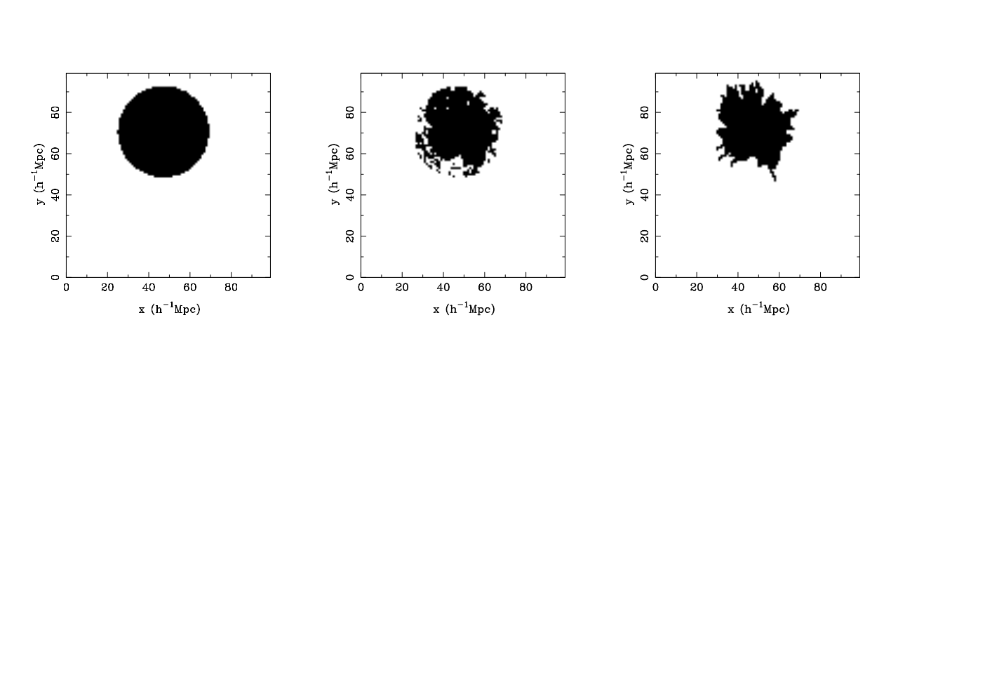
First, we consider the case of a single ionizing source with the ionizing luminosity of a bright QSO in the most massive halo () in the simulation volume as a test case. The ionizing luminosity and the age of the QSO are chosen such that the ionized region has a comoving radius of Mpc within an otherwise completely neutral and homogeneous IGM. This corresponds to an ionized fraction of averaged over the whole simulation volume. Ionization maps for two-dimensional slices centered on the “QSO” are shown in Figure 3 for the case with and without an inhomogeneous spatial distribution of recombinations in the middle and left panels respectively. The right panel shows the same slice with the effects of shadowing taken into account.
In the left panel of the figure where no (or only spatially homogeneous recombinations have been included) the ionized region is spherical with radius as expected for the assumed ionizing luminosity. This confirms that our method of generating ionization fields is reasonably accurate for the case of spatially homogeneous recombinations and justifies our assumption that only the central pixel rather than the whole filtered sphere is ionized.
When the density dependence of recombinations are taken into account allowing high-density regions to stay neutral the appearance of the ionized region is very different due to the then very inhomogeneous spatial distribution of sinks of ionizing radiation. The resulting ionized fraction also decreases from to , despite the fact that the ionizing luminosity of the QSO has the same value as before. This is simply due to the fact that a larger number of photons is needed to overcome the recombinations predominantly occurring in high-density regions. More importantly, the shape of the ionized region is now far from spherical. The ionization fronts appear to progress into the low-density regions while they are halted when high-density clumps are encountered (see the left panel of Figure 1 for the corresponding density field). However, we find that there are some low-density pixels which lie in the shadow of a self-shielded clump but are still ionized. This unphysical “tunnelling” of photons is a limitation of our modelling which does not take into account shadowing effects.
The effect of shadowing is demonstrated in the right panel of Figure 3. In this case we have used a simple ray-tracing algorithm where rays are going out from the source along all directions. For each point along the ray, we check whether the local photon density is sufficient to ionize hydrogen taking into account recombinations, i.e., we check whether a point can or cannot be self-shielded. The ray is terminated once it hits a self-shielding pixel, thus forming a shadow on the other side of the high-density point. The differences in the topology of the resulting field are obvious. The edges of the ionized bubble are more ragged when shadowing is included. Note, however, that the difference in the global ionized fraction is only or about per cent. For representative volumes of the Universe the effect of shadowing will be much less dramatic. Points lying in the shadow of a high-density clump with respect to one ionizing source will generally receive ionizing photons from sources in other directions.
3.2 Modelling representative volumes of the Universe
We now discuss ionization maps of representative volumes of the Universe where significant numbers of haloes (as opposed to a single source) host ionizing sources. In order to investigate the effect of a spatially inhomogeneous distribution of sinks and sources of ionizing radiation and the speed with which reionization occurs we consider four different models:
- •
HR: The spatial distribution of recombinations is assumed to be homogeneous. The condition for a region to be ionized is given by equation (2), with being chosen so as to give a defined global mass-averaged ionized fraction .
- •
IR-0.5: The spatial distribution of recombinations is assumed to be inhomogeneous as discussed in section 2.5. The condition for a region to be ionized is determined by equation (7) [which is same as in the HR model] and the self-shielding condition (15) with a value of . is adjusted to give the same values of for all four models.
- •
IR-1.0: The same as the previous model but with . The effect of recombinations should be more prominent than in the previous model.
- •
IR-HM: The same as model IR-1.0 except that only high mass (HM) haloes with are ionizing sources. This model investigates the possibility that ionizing photons within lower mass haloes may not be able to escape into the IGM efficiently (e.g. [Gnedin (2008]). These small haloes may still form stars, but in this model we assume that the ionizing photons are then absorbed within the interstellar medium and hence the galaxy remains mostly neutral, possibly contributing significantly to the neutral hydrogen budget.
Before investigating the ionization maps generated using the above models, we first discuss the predicted evolution of the global mass-averaged ionized fraction . To obtain the evolution of , we have calculated the collapsed mass fraction using the theoretical Sheth-Tormen mass function assuming a value of as set by our fiducial simulation box. This means that the effects of various feedback processes on star-formation have been ignored. We have then estimated the value of from using the relation for the HR model. For the models with an inhomogeneous spatial distribution of recombinations the above relation was modified to . The values of computed analytically in this way differ from those obtained using the full simulations by up to 15 per cent, however, the basic trends and other conclusions remain unaffected. The corresponding evolution of for the four models is shown in Figure 4. The value of is chosen in each case such that at .
For models HR, IR-0.5 and IR-1.0 (which have the same at a given ), the evolution of is nearly identical. The growth of is slightly more rapid in model IR-1.0 and slightly slower in model HR than in model IR-0.5 , but the differences are small. For the same distribution of haloes, reionization progresses “faster” as the spatially inhomogeneous recombinations become more important. At high-, the average recombination time is shorter than the Hubble time. As a result reionization is less efficient at early epochs when the spatially inhomogeneous recombinations are included. As expected the evolution of is drastically faster in model IR-HM, where only rare massive haloes host ionizing sources. The collapsed fraction in this model is significantly smaller than in the other models, particularly at high redshifts, and hence reionization is initially delayed.
We now discuss the nature of the ionization maps for the different models. Note that we have kept the halo distribution fixed at that corresponding to and have varied the luminosities to obtain different at the same redshift. In reality, however, the variation in is due to the evolution of the halo distribution with redshift. We have here chosen to keep the halo distribution fixed in order to focus on the effect of the different way we treat the spatial distribution of sinks of ionizing radiation in the different models.
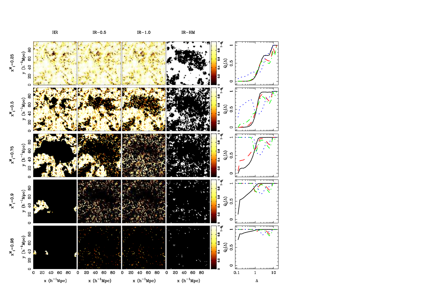
The ionization fields for different are shown in Figure 5 with the left-most panel corresponding to model HR. The second, third and fourth panels describe the three models with a spatially inhomogeneous distribution of sinks of ionizing radiation due to recombinations (IR-0.5, IR-1.0 and IR-HM, respectively). The right-most panel shows the volume-averaged ionized fraction as a function of overdensity . Including the effects of a spatially inhomogeneous distribution of recombinations distinctively changes the topology of ionized regions at fixed ionized mass fraction.
Let us first concentrate on the three columns of panels on the left of Figure 5 corresponding to models HR, IR-0.5 and IR-1.0, respectively. In all three models the ionizing radiation originates from the same dark matter haloes. The models differ only in their treatment of recombinations. To reach the value of , one requires higher values of in models IR-0.5 and IR-1.0 than in model HR as more photons are required to overcome recombination in high-density regions. When the ionized mass fraction is small (), the maps look very similar. At this stage most of the ionizing photons are ionizing the high-density structures which host the photon sources. At the later stages of reionization () , however, the topology of the ionized regions becomes very different in the three models. In model HR the topology of the ionized regions is significantly “smoother” than in the other models. The high-density regions in models IR-0.5 and IR-1.0 remain neutral for longer and hence a larger number of photons per hydrogen atom is required to reach the same . Due to the larger number of ionizing photons per hydrogen atom the ionizing photons are able to reach low-density regions far away from sources of ionizing radiation before the average ionized mass fraction becomes large. The ionization maps of model HR show much larger coherently ionized regions while many neutral (or partially neutral) clumps are embedded within the ionized regions in the models with a spatially inhomogeneous distribution of the sinks of ionizing radiation due to recombinations. In the very late stages of reionization, models IR-0.5 and IR-1.0 are nearly identical.
The dependence of the ionization state on density is shown in the right-most panel; the solid, dashed and dot-dashed curves correspond to models HR, IR-0.5 and IR-1.0, respectively. As already mentioned, early on () the three models are similar, while they start to differ at later stages of reionization. Initially the topology can be described as “inside-out”. High density regions are ionized first. However, in model HR, the ionization of the high-density regions is fully completed before the ionization fronts proceed into the underdense voids, which are the last regions to be ionized. In the HR model reionization proceeds “inside-out” all the way through the reionization process.In models IR-0.5 and IR-1.0, on the other hand, the ionization fronts are trapped by high-density clumps and they therefore proceed into low-density voids leaving behind islands of neutral high-density gas. The topology is now much more complex and cannot be classified simply either as “inside-out” or “outside-in”. Underdense regions () are completely ionized by the time , which is expected as the effect of recombination is negligible within the low-density regions. For regions with , recombinations are important and more than one photon is required to keep the region ionized. The ionized fraction therefore decreases around . Higher overdensities are found close to the filamentary structures in the density field. These regions harbour small mass haloes, i.e,. the relatively faint ionizing sources which are able to overcome recombinations to some extent and are responsible for an increase in the value of around . We have verified this explicitly by computing the collapsed mass fraction within such cells. In even higher density regions, the number of photons required to keep the region ionized becomes much larger than unity and cannot be provided by the fainter sources. Regions with overdensities tend thus to remain neutral. The extremely high-density regions () represent the overlapping of filaments and harbour the most massive/luminous sources. These regions are able to overcome the high recombination rates prevalent there and hence can remain ionized.
The ionization maps of model IR-HM is very similar to those of model IR-0.5 and IR-1.0. The reversal to reionization progressing more “outside-in” occurs somewhat earlier, which is most obvious when investigating the rightmost column showing the ionization state as a function of density (dotted curves). In model IR-HM the ionizing sources reside in rare massive dark matter haloes. A significant number of high-density regions of moderate mass are devoid of any ionizing photon sources locally and are able to remain self-shielded from ionizing photons. This is very different from model IR-0.5 and IR-1.0 where almost all the high-density regions host ionizing sources and hence cannot remain completely neutral. Also note that the behaviour of for intermediate overdensities is somewhat different from that in models IR-0.5 and IR-1.0. There is no peak around in model IR-HM. Recall that the peak in the other models is due to the fainter sources present within filamentary structures. These low-mass sources are absent in model IR-HM and hence the corresponding peak in does not appear.
At this point, let us briefly compare our results with other published results, particularly regarding the typical value of overdensities which can remain self-shielded. For example, ?) have shown, using modelling based on ?), that an overdensity at would be self-shielded only if the local photoionization rate , where is the photoionization rate in units of s-1. We have explicitly verified whether this condition is satisfied in every self-shielded region by estimating using equation (13). We find considerable fluctuations in the local value of (which as expected decreases as reionization progresses and the mean free path rises) and there do remain regions where is much lower than what is required to overcome the self-shielding. To give an explicit example, for the IR-1.0 scenario, we find that regions far away from sources have as low as 0.002 for when the global mean is . The range of values of is typically larger than that found by ?), which is probably due to the difference in the space density of ionizing sources (the smallest haloes in the simulations of ?) have a mass of , while our mass threshold is ).
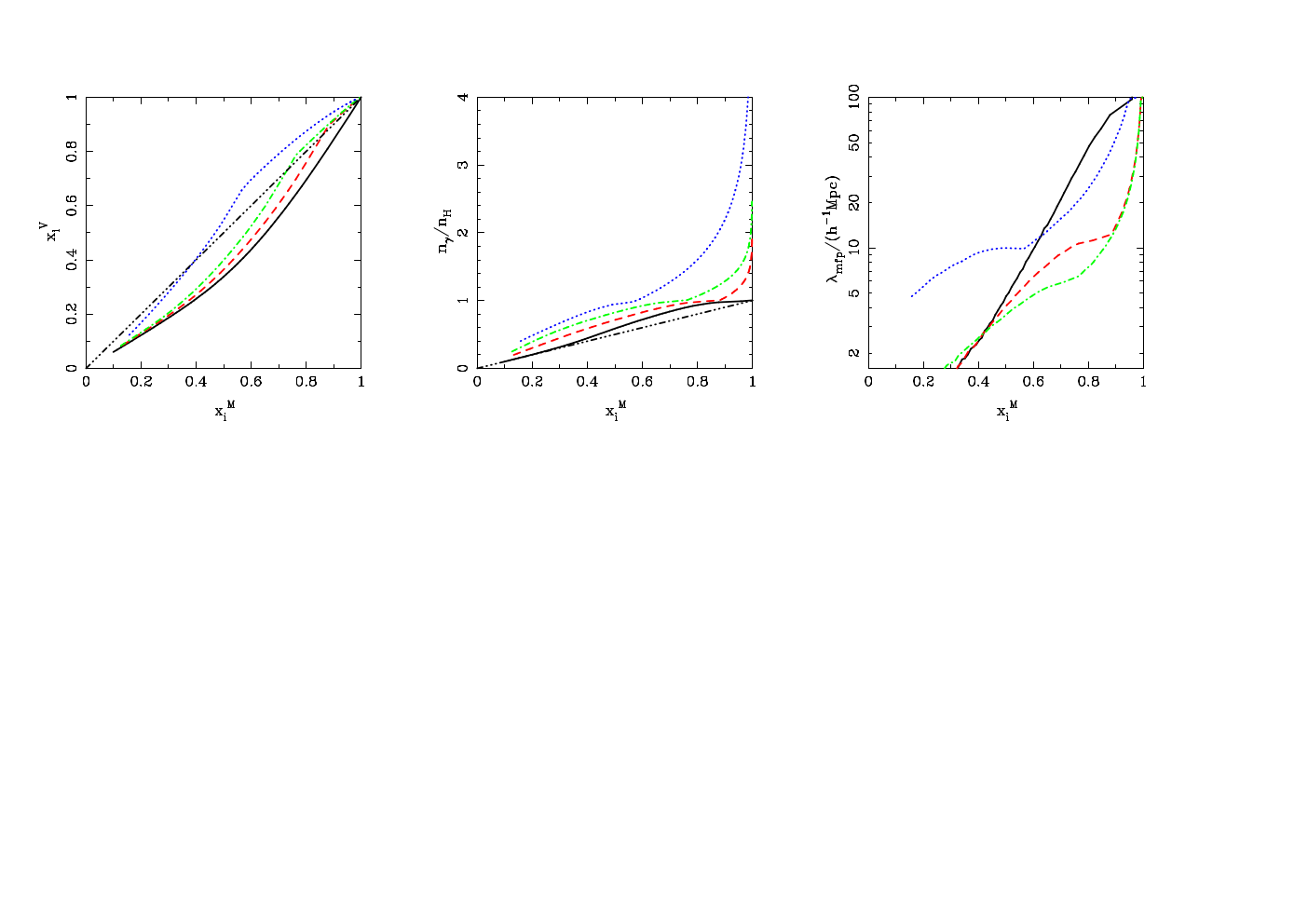
Having demonstrated that reionization should not progress in a simple “inside-out” manner when the inhomogeneous distribution of recombinations is taken into account, we now discuss various other quantities of interest for the different models. The dependence of these quantities on is shown in Figure 6.
The left panel shows the volume-averaged ionized fraction . In the HR model (solid curve) the ionized volume fraction does not exceed the ionized mass fraction () for the whole range of confirming that ionization is biased towards high-density regions. The models with a spatially inhomogeneous distribution of recombinations have in the early stages of reionization (i.e., low values of ), while the trend reverses later on. This is in line with what we discussed earlier, i.e., reionization proceeds “inside-out” at early stages while the situation is more complex later. As expected the reversal of trend occurs earlier in the IR-HM model than in the IR-0.5 and IR-1.0 models. The values of are higher in the IR-HM model than in the IR-1.0 model for given . High density regions are, on average, more neutral in model IR-HM, hence a larger volume has to become ionized to reach the same . Note that for large ionized mass fraction (say ) our models will increasingly underestimate the ionized volume fraction due to insufficient resolution.
The middle panel shows the number of ionizing photons per hydrogen atom reaching the IGM. The first point to be noted is that closely follows the ionized fraction in model HR. Deviations arising from a moderate violation of photon conservation of our algorithm for identifying ionized region are per cent. Obviously, the ratio is higher than for the other models where sinks of ionizing radiation due to recombinations are included. Extra photons are required to reach the same ionized mass fraction. The other crucial difference between model HR and the other three models is that for large ionized mass fractions flattens for model HR while it steepens when inhomogeneous recombinations are included. In model HR low-density voids are the last regions to be ionized and hence the ionized volume increases without significant further need for photons. The situation is exactly opposite for the other cases where most of the photons are being absorbed within high-density regions (acting as “sinks”) and hence no significant rise in is found even though the number of photons used up increases rapidly.
Finally, we plot the dependence of the mean free path in the right panel. To calculate , we first randomly choose a ionized pixel and calculate the distance to a neutral pixel along a randomly chosen direction; this should denote the local mean free path for the chosen point. This Monte Carlo procedure is repeated for a large number of points. The global mean free path is then estimated in two different ways: (i) is estimated as the average of the different local mean free paths and (ii) is estimated as the median of the local mean free path distribution. In most cases, both methods give nearly identical estimates. The curves plotted in the figure are obtained using the median [method (ii)].
The dependence of on the ionized mass fraction is most easily understood in the HR model (solid curve) where it is determined by the characteristic size of ionized regions. rises with essentially featureless until it flattens when approaches the size of the simulation box. The trends for models IR-0.5 (dashed curve) and IR-1.0 (dot-dashed curve) are similar to that in model HR in the early stages of reionization (). However, as reionization progresses, the mean free path in models IR-0.5 and IR-1.0 is smaller than that in the HR model. High density clumps limit the propagation of ionizing photons in these models. The mean free path in the models with spatially inhomogeneous recombination is thus not determined by the sizes of ionized regions when is large. It depends instead on the spatial covering factor of high-density peaks. Note that the mean free path in the IR-HM model is larger than that in the IR-0.5 and IR-1.0 models for given . This is consistent with the fact in these models a larger volume has to be ionized to reach the same ionized mass fraction. Note the “break” in the evolution of for the models with inhomogeneous recombinations. This break broadly defines the epoch when the mean free path starts to be limited by high-density clumps rather than the size of ionized regions.
We should mention here that is likely that we have overestimated the sizes of the self-shielded absorbers because of the limited spatial resolution of our simulations This should lead to an underestimate of . The limited resolution will, however, at the same time, result in an underestimate of the space density of self-shielded regions as well as of recombination outside of self-shielded absorbers. This should in turn have lead to an overestimate of the mean free path. The two effects should thus partially cancel. We have examined the effect of resolution on in Appendix B and found that our results do not change when the resolution is improved by a factor of two. The absolute values of the mean free path shown in figure 6 should nevertheless be treated with some caution but our finding that the mean free path will evolve more slowly if recombinations are important should be robust.
4 Consistency with Ly forest data at
Current observational constraints on the epoch of reionization are still rather limited. Studies of the Ly forest in QSO absorption spectra have taught us that reionization probably ended at around ([Fan et al. (2002, Fan et al. (2004, Fan et al. (2006]; cf [Becker, Rauch, & Sargent (2007]). As discussed by ?) and ?), the emissivity inferred from the Ly forest data corresponds to at most a few photons per hydrogen atom per Hubble time. ?) thus coined the term “photon-starved” to describe the regime in which reionization appears to occur. ?) measured the emissivity of ionizing photons to be roughly constant in comoving units in the redshift range . They pointed out that because of the rather low emissivity of ionizing photons reionization of hydrogen most likely started early and extends over a wide redshift range. This sits well with the rather large Thomson optical depth inferred from studies of the cosmic microwave background [Spergel et al. (2007, Dunkley et al. (2008, Choudhury, Ferrara, & Gallerani (2008]. Predictions of ionization maps should obviously be consistent with available data. Enforcing consistency with the Ly forest data shrinks the allowed parameter space considerably and we therefore discuss now how our modelling fairs in this respect.
In Table 1 we summarize the mean-free path of ionizing photons and the inferred photoionization rate in our three models for two values of the volume fraction of ionized regions (at ) and two different assumptions for when reionization has started at and , respectively. The value of the mean free path of ionising photons and the volume fraction of ionized regions at are observationally still very uncertain. ?) estimate the mean free path to be and infer a photoionization rate . The volume fraction of ionized regions has been estimated to be at from the evolution of Ly luminosity function [Kashikawa et al. (2006] and GRB spectrum [Totani et al. (2006], while the constraints from QSO absorption line measurements at are quoted to give [Fan et al. (2006].
For our models with a spatially inhomogeneous distribution of recombinations the mean free path is reasonably consistent with the estimate of ?) if the volume fraction of ionized regions is large (95%). For models HR and IR-HM on the other hand, the estimated mean free path is consistent with the values in Table 1 if the volume fraction of ionized regions at is low (50%).
We have estimated the photoionization rate (in units of s-1) inferred from the photon emission rate and using [Bolton & Haehnelt (2007],
| (16) | |||||
where is the spectral index of the ionizing background (which we assume to be 3 consistent with stellar sources of sub-solar metallicity). The results are shown in the two right-most columns in table 1. Note again that there could be inaccuracies of per cent arising from moderate violations of photon conservation of our algorithm. For models IR-0.5 and IR-1.0 we find reasonable agreement with the inferred photoionization rate for . On the other hand, models HR and IR-HM generally tend to overpredict the photoionization rate when the assumed ionized fraction is large. For smaller values of the ionized mass fraction (), these models are found to be consistent with the data.
| Model | |||||
|---|---|---|---|---|---|
| HR | 0.5 | 15 | 0.79 | 0.031 | 0.044 |
| 0.95 | 97 | 0.96 | 0.257 | 0.362 | |
| IR-0.5 | 0.5 | 8 | 0.82 | 0.016 | 0.023 |
| 0.95 | 21 | 1.14 | 0.063 | 0.089 | |
| IR-1.0 | 0.5 | 5 | 0.89 | 0.011 | 0.015 |
| 0.95 | 21 | 1.40 | 0.076 | 0.107 | |
| IR-HM | 0.5 | 12 | 0.91 | 0.026 | 0.036 |
| 0.95 | 56 | 2.20 | 0.330 | 0.465 | |
5 Predictions for 21cm observations
5.1 The effect of the spatial distribution of sinks and the luminosity of sources on the 21cm power spectrum.


We have seen in Section 3.2 that the models with different assumptions regarding the spatial distribution of sinks and sources of ionizing radiation predict rather different topologies for the neutral hydrogen distribution, particularly in the late stages of reionization (with the exception that models IR-0.5 and IR-1.0 are nearly identical for ). We now discuss the prospects of investigating the effects of the spatial distribution of the sinks and sources of ionizing radiation with future low-frequency radio observations of the redshifted 21cm line. Since model IR-0.5 is qualitatively very similar to model IR-1.0, we shall not discuss it separately in this section.
The 21cm brightness temperature at a given location relative to the CMB can be approximated as
| (17) |
where we have assumed that the spin temperature of hydrogen is much larger than the CMB temperature. This should be a reasonable assumption once a significant fraction (a few percent) of the volume/mass has been ionized ([Scott & Rees (1990, Tozzi et al. (2000, Ciardi & Madau (2003, Barkana & Loeb (2005, Sethi (2005, Furlanetto (2006, Furlanetto, Oh, & Briggs (2006]; see [Pritchard & Loeb (2008] for an extensive recent discussion of the expected evolution of the spin temperature). We have also ignored peculiar velocity effects which are small at the scales relevant here (see, e.g., [Mesinger & Furlanetto (2007]). The quantity denotes the brightness temperature for neutral gas at mean density. By definition, .
The first quantity of interest is the power spectrum of temperature fluctuations which we define as . The power spectrum is plotted in Figure 7 for our models for a range of values of (e.g. [Furlanetto, Zaldarriaga, & Hernquist (2004a]). The panels from left to right show the power spectrum for models HR, IR-1.0 and IR-HM, respectively. In each panel the power spectrum is shown for mass-averaged ionization fraction 0 (solid), 0.1 (dashed), 0.3 (dot-dashed), 0.5 (dotted), 0.7 (dot-dot-dot-dashed) and 0.9 (triangles) respectively. For , the brightness temperature simply traces the DM fluctuations.
In model HR (left panel), the amplitude of the power spectrum decreases from its initial value until about (dot-dashed curve). The decrease of the fluctuation amplitude, particularly at large scales, occurs as regions of high density become ionized. The decrease in amplitude is accompanied by a steepening in slope, consistent with the findings of ?). It follows then a reversal in trend. The amplitude rises (particularly at large scales Mpc-1) and the slope becomes shallower. This is particularly evident if the power spectra for (dot-dashed curve) and (dotted curve) are compared. This is the phase when the the ionizing radiation from collapsed objects ionizes the surrounding high-density regions. The growth of ionized regions boosts the large scale power and flattens the slope of . The flattening of the slope continues (and the power spectrum becomes practically flat) as the IGM becomes more ionized while the amplitude decreases at high values of . In model HR there is nearly equal power at all scales in the late stages of reionization and the fluctuation amplitude decreases as the neutral hydrogen content in the IGM decreases.
In the early stages of reionization () the evolution of the 21cm power spectrum in model IR-1.0 (middle panel) is very similar to that in model HR. The similarity, however, disappears for when the slope of steepens rather than flattens. The high-density neutral regions embedded within the ionized regions are responsible for a considerable amount of small-scale power in the 21cm power spectrum. At the same time, the clumps limit the size of coherently ionized regions, thus keeping the large-scale power low. This pattern holds until the very end of reionization. The steepening of the slope in the later stages of reionization in the models with an inhomogeneous spatial distribution of recombinations is a signature of the more complex topology which we had described in section 3.2. In the late stages reionization proceeds much more “outside-in” than in model HR and this is clearly recognizable in the 21cm power spectra.
A similar but more pronounced steepening of the slope of the 21cm power spectrum occurs in model IR-HM, where the emission of ionizing photons is restricted to massive haloes. Here reionization starts to proceed in a more “outside-in” fashion much earlier. The behaviour of the amplitude 21cm spectrum at large scales () is less complicated than in the other two models; there is a slight dip in the power spectrum around due to the ionization of the high-density regions harbouring the sources of ionizing radiation. Otherwise the power spectrum evolves very little until and then the amplitude decreases with decreasing neutral fraction. In model IR-HM the amplitude of the 21cm power spectrum is generally somewhat higher than in the other two models. This is due to reionization being driven by relatively highly clustered sources in this model.
5.2 Evolution of slope and amplitude of the 21cm power spectrum at scales probed by LOFAR and MWA
In the last section we developed a feeling for how the spatial distribution of sinks and sources of ionizing radiation influence the 21cm power spectrum. We now discuss in more detail the possibility to differentiate observationally between different models with first generation 21cm experiments like LOFAR and MWA. The typical scales probed by these experiments correspond to wavenumbers . Foreground subtraction will be a serious problem and it is not clear yet to how small and large scales it will be possible to determine the power spectrum with reasonable accuracy. We follow ?) and assume that the optimum scale for studying 21cm fluctuations with these instruments correspond to and use a pivot scale of in the following to be definite. This scale is well suited for a discrimination between our models.
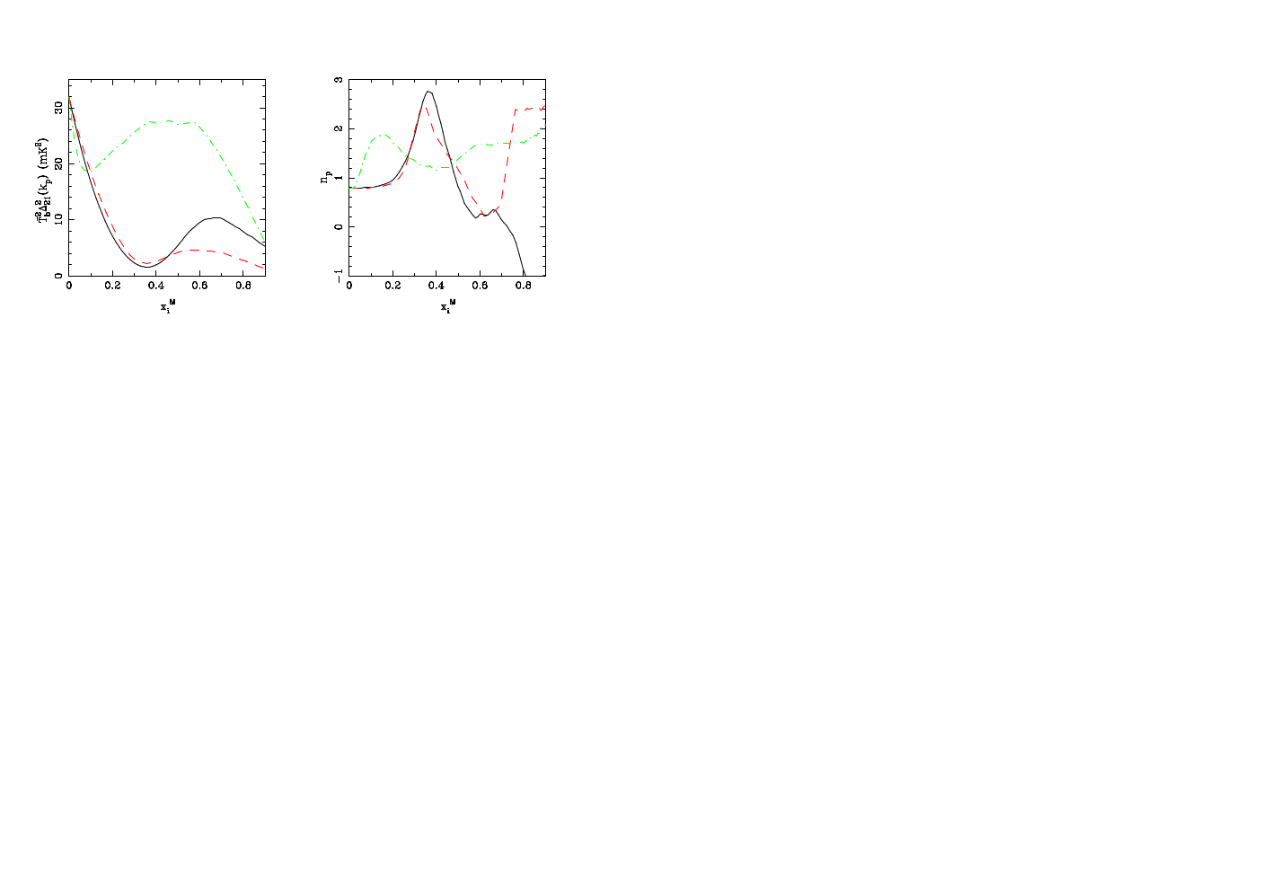
The amplitude of the power spectrum at and its slope as a function of the ionized mass fraction are shown in the left and right panels of Figure 8. The evolution of the different models reflects our discussion in the last section. The evolution of the amplitude can be divided into three phases. An initial decrease in amplitude due to the early ionization of high-density regions ([Wyithe & Morales (2007]), is followed by a rise corresponding to a growth in patchiness and a final fall due to the elimination of neutral hydrogen. In model HR-IM (dot-dashed curve) where reionization is driven by rarer sources the 21cm power spectrum has significantly (a factor two or more) power than in the other two models. The amplitude of the power spectrum and its evolution at our pivot scale contains valuable information about the spatial distribution of ionizing sources.
The amplitude of the power spectrum at our pivot scale appears, however, not to be a good indicator of the spatial distribution of the sinks of ionizing radiation. Models HR and IR-1.0 models are very similar in this respect. As discussed earlier the spatial distribution of sinks has instead a strong influence on the slope of the power spectrum (right panel). The evolution of the slope can be again divided into three phases. An initial rise due to the ionization of high-density regions followed by a fall corresponding to the growth of patchiness. In the third phase at keeps on decreasing rapidly in the HR model while it increases instead in the models with a spatially inhomogeneous distribution of sinks of ionizing radiation due to recombinations.
By measuring the power spectrum and its slope at large scales () it should thus be possible to characterize both the spatial distribution of sources and sinks of ionizing radiation. The detectability of the 21cm fluctuations obviously depends on the instrument noise and the ability to subtract foreground emission. Assuming a perfect removal of foreground emission ?) find typical values of detector noise for LOFAR and MWA at of mK2 at for 1000 hrs of observation. With such noise levels, the power spectra for the HR and the IR-HM models should be detectable with reasonable confidence in the range and ,respectively. The fluctuation amplitude in model IR-1.0 is lower than in the other two models discussed in this section. At their peak value around 21cm fluctuations should nevertheless be detectable by LOFAR and MWA even for this model. Note that the values quoted here should be only taken as indicative. Both the noise properties and the fluctuation amplitude depend on redshift For example in our models an ionized mass fraction of is reached around while our estimations were performed assuming .
5.3 The PDF of the 21cm brightness distribution
We now briefly discuss the probability distribution of the dimensionless brightness temperature [Furlanetto, Zaldarriaga, & Hernquist (2004b]. In order to compute the distribution, we smooth the brightness temperature over scales of Mpc, as is appropriate for the first generation 21cm experiments. The results are shown in Figure 9. The left panel shows the 21cm PDF for model HR. The curves with peaks from right to left are for , respectively. We have chosen the values of such that they represent the characteristic points in the evolution of the power spectrum at large scales. The curve for (solid) obviously represents the dark matter PDF. For (dashed curve), the PDF has become significantly narrower. This is again due to the ionization of high-density regions and corresponds to a low-amplitude of the power spectrum. The evolution of the PDF in model HR is consistent with the analytical models of ?). The PDF widens subsequently with increasing as more regions are being ionized. The behaviour is similar in model IR-1.0 (middle panel) where the curves with peaks from right to left represent , respectively. The only difference is a somewhat narrower width of the distribution than in model HR in the final stages of reionization (). This is consistent with what is expected from the evolution of the 21cm power spectra at large scales. The results for model IR-HM are shown in the right panel. The curves with peaks from right to left represent , respectively. As expected, the PDF in this model is rather different from that in the other two models. The PDF in model IR-HM has a wider distribution compared to the other two models. The model predicts even when the IGM is 50 per cent ionized by mass. Unfortunately, it is not clear whether the first generation 21 cm experiments will have enough sensitivity to constrain the shape of the PDF.
5.4 Comparison with other work
As discussed in the introduction, there has been a number of recent studies which aim at predicting the 21cm brightness distribution. These studies range from radiative transfer simulation generally performed by post-processing the density field of DM simulations [Ciardi, Ferrara, & White (2003, Iliev et al. (2006b, Mellema et al. (2006, Iliev et al. (2007, McQuinn et al. (2006, McQuinn et al. (2007, Zahn et al. (2007] to semi-numerical simulations [Mesinger & Furlanetto (2007, Alvarez & Abel (2007, Geil & Wyithe (2008] similar in spirit to the work presented here. Most of these studies appear to agree that reionization occurs inside-out all the way from the start until nearly the completion of reionization. ?) have thereby shown that results for semi-numeric schemes based on collapsed mass fractions and variants of the excursion set formalism to identify regions which can self-ionize give very similar results to full radiative transfer simulations if similar assumptions regarding the sources of ionizing radiation are made. Most similar to our work here is probably the work of ?) who have studied a wide range of assumptions regarding the sources and sinks of ionizing radiation. When modelling the effects of sinks of ionizing radiation ?) mainly study mini-haloes, dark matter haloes with potential wells shallow enough so that they can be photo-evaporated by ionizing photons. For these mini-haloes they find a noticeable but rather small effect (see [Bolton & Haehnelt (2007] for a brief discussion of the role of mini-haloes during reionization in the photon-starved regime). ?), however, do not try to model recombinations in high-density regions in deeper potential wells which can hold on to photo-ionized gas in a way so that their models are likely to be consistent with the Ly forest data. They generally find that sinks of ionizing radiation and their spatial distribution have little effect on the topology of reionization and the power spectrum. This is obviously quite different from our findings. There is a number of differences to our modelling but the most likely reason appears to be the following. The emissivity used in the models of ?) is rather high and reionization proceeds quickly. This strongly diminishes the importance of recombination compared to our modelling of reionization in the photon-starved regime suggested by the Ly forest data.
6 Conclusions
We have used here semi-numerical simulations to investigate the role of the spatial distribution of sinks and sources of ionizing radiation on the topology of hydrogen reionization. Our main results are the following.
- •
The combination of Zel’dovich approximation, halo-finder and excursion set formalism is a powerful tool to calculate realistic ionization maps with high dynamic range at a very moderate computational cost.
- •
Enforcing consistency with the Ly forest data helps to significantly shrink the otherwise rather unconstrained parameter space of models of reionization. In the photon-starved regime of reionization suggested by the Ly forest data recombinations are much more important than in models with high ionizing emissivity where reionization occurs quickly. Taking into account a realistic spatially inhomogeneous distribution of sinks of ionizing radiation has a large effect on the topology of reionization in the photon-starved regime.
- •
Initially reionization proceeds inside-out with the high-density regions hosting the sources of ionizing sources becoming ionized first. In the later stages of photon-starved reionization the sinks of ionizing region in our models remain neutral and reionization proceeds deep into the underdense regions before slowly evaporating denser regions not hosting ionizing sources where recombinations are important. This reversal to a more outside-in progression in the late stages of reionization is more pronounced if the emission of ionizing radiation is restricted to massive highly-clustered and rare sources.
- •
If the emission of ionizing radiation is restricted to rare sources reionization proceeds more quickly and the sizes of coherently ionized regions are significantly larger. The latter results in an about factor two or more larger mean free path for ionizing photons.
- •
Like other studies we find that the amplitude of the 21cm power spectrum and its evolution in the later stages of reionization is mainly sensitive to the space density of ionizing sources. The sensitivity to the space density of ionizing sources is, however, significantly increased if a realistic spatially inhomogeneous distribution of sinks of ionizing radiation is taken into account. The slope of the power spectrum is very sensitive to the spatial distribution of sinks of ionizing radiation.
- •
Measurements of the amplitude and slope of the 21cm power spectrum at scales corresponding to with the upcoming low-frequency instruments LOFAR and MWA have excellent prospects to reveal important information on the spatial distribution of sinks and sources of ionizing radiation and the speed of reionization if the daunting tasks of accurate calibration and foreground removal are mastered successfully. The PDF of the 21cm brightness distribution contains important complimentary information. Measuring the PDF will, however, unfortunately most likely require higher sensitivity than can be achieved with first generation 21cm experiments.
Our modelling here has involved a number of significant simplifications. The spatial distribution of dark matter modelled in the Zel’dovich approximation was used as an proxy for the spatial distribution of the IGM. The ionizing emissivity of sources and recombination in dense region was modelled only in an approximate integrated fashion and the dynamical effects of the ionization radiation on the gas were neglected. Despite the large particle number used in the simulations resulting in a substantial dynamic range there were still clear deficiencies in modelling high-density regions and low-mass collapsed objects/mini-haloes. We nevertheless think that our simulations have caught the essential properties of the topology of the epoch of reionization. Our simulations suggest that the idea that reionization proceeds strictly inside-out from beginning to nearly to the end may need revision if reionization indeed occurs in a photon-starved regime as suggested by the Ly forest data.
Acknowledgments
We thank Tom Abel, Benedetta Ciardi, Nick Gnedin, Ilian Iliev, Adam Lidz, Avi Loeb, Matthew McQuinn, Jordi Miralda-Escudé and Paul Shapiro for valuable comments made at the 2008 Harvard conference on 21cm Cosmology where part of this work was presented. This research was conducted in cooperation with SGI/Intel utilizing the Altix 4800 supercomputer COSMOS at the Department of Applied Mathematics and Theoretical Physics in Cambridge. COSMOS is a UK-CCC facility which is supported by HEFCE and STFC/PPARC. Part of the simulations where performed on the Cambridge High Performance Computing Cluster Darwin.
References
- Alvarez & Abel (2007 Alvarez M. A., Abel T., 2007, MNRAS, 380, L30
- Barkana & Loeb (2005 Barkana R., Loeb A., 2005, ApJ, 626, 1
- Becker, Rauch, & Sargent (2007 Becker G. D., Rauch M., Sargent W. L. W., 2007, ApJ, 662, 72
- Bolton & Haehnelt (2007 Bolton J. S., Haehnelt M. G., 2007, MNRAS, 382, 325
- Chen, Prochaska, & Gnedin (2007 Chen H.-W., Prochaska J. X., Gnedin N. Y., 2007, ApJ, 667, L125
- Choudhury & Ferrara (2005 Choudhury T. R., Ferrara A., 2005, MNRAS, 361, 577
- Choudhury & Ferrara (2006a Choudhury T. R., Ferrara A., 2006a, in Cosmic Polarization , ed. R. Fabbri (Research Signpost) (astro-ph/0603149), p. 205
- Choudhury & Ferrara (2006b Choudhury T. R., Ferrara A., 2006b, MNRAS, 371, L55
- Choudhury, Ferrara, & Gallerani (2008 Choudhury T. R., Ferrara A., Gallerani S., 2008, MNRAS, 385, L58
- Ciardi, Ferrara, & White (2003 Ciardi B., Ferrara A., White S. D. M., 2003, MNRAS, 344, L7
- Ciardi & Madau (2003 Ciardi B., Madau P., 2003, ApJ, 596, 1
- Davis et al. (1985 Davis M., Efstathiou G., Frenk C. S., White S. D. M., 1985, ApJ, 292, 371
- Dunkley et al. (2008 Dunkley J. et al., 2008, Preprint, arXiv:0803.0586
- Fan et al. (2004 Fan X. et al., 2004, AJ, 128, 515
- Fan et al. (2002 Fan X., Narayanan V. K., Strauss M. A., White R. L., Becker R. H., Pentericci L., Rix H., 2002, AJ, 123, 1247
- Fan et al. (2006 Fan X. et al., 2006, AJ, 132, 117
- Furlanetto (2006 Furlanetto S. R., 2006, MNRAS, 371, 867
- Furlanetto & Oh (2005 Furlanetto S. R., Oh S. P., 2005, MNRAS, 363, 1031
- Furlanetto, Oh, & Briggs (2006 Furlanetto S. R., Oh S. P., Briggs F. H., 2006, Phys. Rep., 433, 181
- Furlanetto, Zaldarriaga, & Hernquist (2004a Furlanetto S. R., Zaldarriaga M., Hernquist L., 2004a, ApJ, 613, 16
- Furlanetto, Zaldarriaga, & Hernquist (2004b Furlanetto S. R., Zaldarriaga M., Hernquist L., 2004b, ApJ, 613, 1
- Geil & Wyithe (2008 Geil P. M., Wyithe J. S. B., 2008, MNRAS, 386, 1683
- Gnedin (2000 Gnedin N. Y., 2000, ApJ, 535, 530
- Gnedin (2008 Gnedin N. Y., 2008, ApJ, 673, L1
- Gnedin, Kravtsov, & Chen (2008 Gnedin N. Y., Kravtsov A. V., Chen H.-W., 2008, ApJ, 672, 765
- Iliev et al. (2006a Iliev I. T. et al., 2006a, MNRAS, 371, 1057
- Iliev et al. (2006b Iliev I. T., Mellema G., Pen U.-L., Merz H., Shapiro P. R., Alvarez M. A., 2006b, MNRAS, 369, 1625
- Iliev et al. (2007 Iliev I. T., Mellema G., Shapiro P. R., Pen U.-L., 2007, MNRAS, 376, 534
- Inoue, Iwata, & Deharveng (2006 Inoue A. K., Iwata I., Deharveng J.-M., 2006, MNRAS, 371, L1
- Jenkins et al. (2001 Jenkins A., Frenk C. S., White S. D. M., Colberg J. M., Cole S., Evrard A. E., Couchman H. M. P., Yoshida N., 2001, MNRAS, 321, 372
- Kashikawa et al. (2006 Kashikawa N. et al., 2006, ApJ, 648, 7
- Lidz et al. (2008 Lidz A., Zahn O., Furlanetto S., McQuinn M., Hernquist L., Zaldarriaga M., 2008, Preprint, arXiv:0806.1055
- Lidz et al. (2007 Lidz A., Zahn O., McQuinn M., Zaldarriaga M., Hernquist L., 2007, Preprint: arXiv:0711.4373
- McQuinn et al. (2007 McQuinn M., Lidz A., Zahn O., Dutta S., Hernquist L., Zaldarriaga M., 2007, MNRAS, 377, 1043
- McQuinn et al. (2006 McQuinn M., Zahn O., Zaldarriaga M., Hernquist L., Furlanetto S. R., 2006, ApJ, 653, 815
- Mellema et al. (2006 Mellema G., Iliev I. T., Pen U.-L., Shapiro P. R., 2006, MNRAS, 372, 679
- Mesinger & Dijkstra (2008 Mesinger A., Dijkstra M., 2008, MNRAS, 390, 1071
- Mesinger & Furlanetto (2007 Mesinger A., Furlanetto S., 2007, ApJ, 669, 663
- Miralda-Escudé (2003 Miralda-Escudé J., 2003, ApJ, 597, 66
- Miralda-Escudé, Haehnelt, & Rees (2000 Miralda-Escudé J., Haehnelt M., Rees M. J., 2000, ApJ, 530, 1
- Monaco et al. (2002 Monaco P., Theuns T., Taffoni G., Governato F., Quinn T., Stadel J., 2002, ApJ, 564, 8
- Paschos & Norman (2005 Paschos P., Norman M. L., 2005, ApJ, 631, 59
- Pritchard & Loeb (2008 Pritchard J. R., Loeb A., 2008, Preprints, arXiv:0802.2102
- Schaye (2001 Schaye J., 2001, ApJ, 559, 507
- Scoccimarro & Sheth (2002 Scoccimarro R., Sheth R. K., 2002, MNRAS, 329, 629
- Scott & Rees (1990 Scott D., Rees M. J., 1990, MNRAS, 247, 510
- Sethi (2005 Sethi S. K., 2005, MNRAS, 363, 818
- Sheth & Tormen (2002 Sheth R. K., Tormen G., 2002, MNRAS, 329, 61
- Spergel et al. (2007 Spergel D. N. et al., 2007, ApJS, 170, 377
- Springel et al. (2005 Springel V. et al., 2005, Nat, 435, 629
- Totani et al. (2006 Totani T., Kawai N., Kosugi G., Aoki K., Yamada T., Iye M., Ohta K., Hattori T., 2006, PASJ, 58, 485
- Tozzi et al. (2000 Tozzi P., Madau P., Meiksin A., Rees M. J., 2000, ApJ, 528, 597
- Viel, Haehnelt, & Lewis (2006 Viel M., Haehnelt M. G., Lewis A., 2006, MNRAS, 370, L51
- Wyithe & Loeb (2003 Wyithe J. S. B., Loeb A., 2003, ApJ, 586, 693
- Wyithe & Loeb (2007 Wyithe J. S. B., Loeb A., 2007, MNRAS, 375, 1034
- Wyithe & Morales (2007 Wyithe J. S. B., Morales M. F., 2007, MNRAS, 379, 1647
- Zahn et al. (2007 Zahn O., Lidz A., McQuinn M., Dutta S., Hernquist L., Zaldarriaga M., Furlanetto S. R., 2007, ApJ, 654, 12
Appendix A Comparison of different methods of generating the halo field
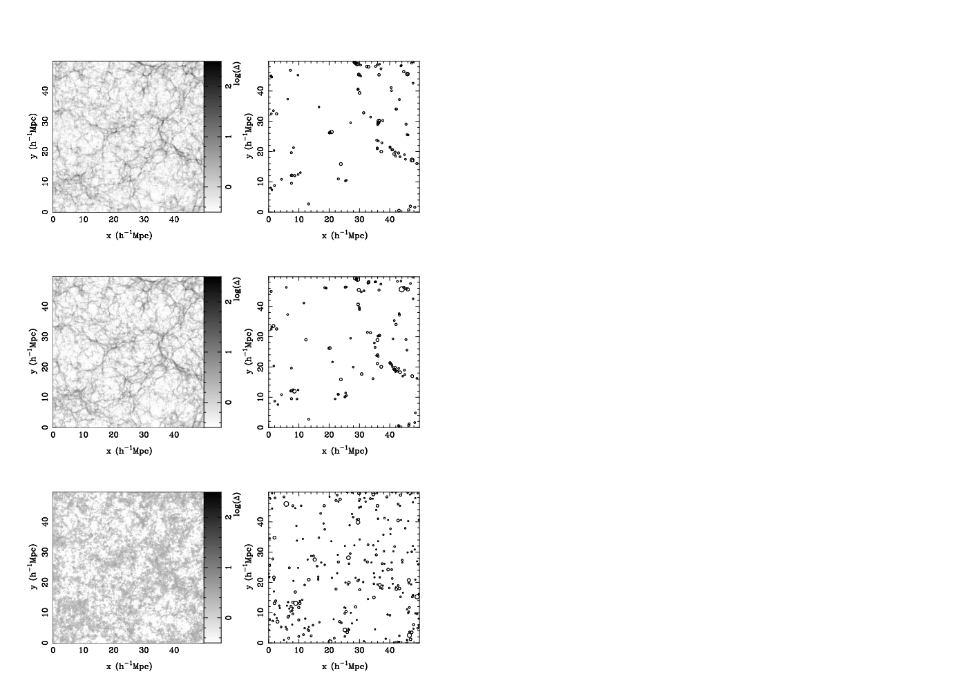

In this Appendix, we compare three different ways of generating the density field and locating haloes within the simulation volume. Dark matter haloes were identified for density distributions with identical initial conditions within a simulation box of comoving length 50 Mpc with particles, giving a mass resolution of . For definiteness, we concentrate our comparison on (which is the fiducial redshift of study throughout the paper).
- •
N-body + FoF: In this approach, the dark matter density field is generated by running a full N-body simulation (with GadgetII) and then a standard Friends-of-friends (FoF) algorithm with linking length times the mean inter-particle separation is applied to find the haloes. Typically, one is able to identify haloes as small as times the mass resolution which are consistent with theoretical predictions of halo mass function. This is most accurate method to obtain the spatial distribution of dark matter haloes. The disadvantage is that in order to achieve the dynamic range required for studying reionization is generally computationally expensive (both in terms of CPU time and memory). The density field and the location of dark matter haloes obtained in this way are shown in the top panels of Figure 10.
- •
ZA + FoF: An alternate method of generating the density field is the Zel’dovich approximation. In this case, we have generated the density field at a given redshift by displacing the particles from their initial positions using the linear velocity field. This procedure is significantly less computationally expensive than a N-body simulation and nevertheless gives give a reasonable representation of the density field at high redshifts. The location and mass of the haloes was then obtained with FoF halo finder with a variable linking length with . The detailed internal structure of the haloes is not correct in this case (the density profiles of the haloes is generally much more diffuse and the halo particle may even not not be bound). However, these details are not important for our work here where we want to investigate qualitatively the topology of reionization. The density field and the location of the haloes obtained in this way are shown in the middle panels of Figure 10. One immediately appreciates that the visual impression of both the density structure and halo field generated by this approach is very similar to the previous one, the differences being rather minor.
- •
GRF + ES: The third method we have explored is evolving the initial Gaussian random field (GRF) linearly (i.e., multiplying by the appropriate growth factor) and applying the excursion set (ES) formalism to identify the haloes. The advantage in this case is that the formalism is computationally very cheap and can identify haloes as small as the mass resolution of the box. The disadvantage is that the linear density field does not necessarily capture the true density distribution which is a serious problem for the analyses presented here. The results obtained by this approach are shown in the bottom panels of Figure 10. It is immediately apparent that the density structure is drastically different from the previous two approaches with no apparent filamentary networks visible. The same is true for the location of the haloes (though it should be mentioned that the number of haloes identified are much larger than the previous methods as one can locate smaller haloes). A better match with the simulations can be achieved if both the densities and halo positions are adjusted using the Zel’dovich approximation [Zahn et al. (2007, Mesinger & Furlanetto (2007]; however it is not clear how well the density peaks would correspond to halo locations if both are displaced independently. Since a reasonable representation of the density field and location of the haloes are vital for our work here, this very simple computationally least expensive scheme is unfortunately not appropriate for this work.
The fact that the “ZA + FoF” method gives a reasonable approximation of the density and halo field can also be seen quantitatively from Figure 11 where we have plotted the volume-weighted density distribution (left panel) and the power spectrum of density fluctuations (right panel) for the three methods. The density distribution obtained with the “ZA + FoF” method (dashed curve) closely resembles that obtained with “Nbody + FoF” (solid curve), which is quite different from the gaussian distribution (dot-dashed curve) obtained with the “GRF + ES” method. Similarly, the plots of the power spectrum shows that the “GRF + ES” method deviates from the “Nbody + FoF” at scales Mpc, while the “ZA + FoF” method is reasonable down to scales of a few Mpc. At smaller scales, the “Nbody + FoF” method generates more power than the other two cases due to a correct treatment of non-linearities. It appears thus fair to say that the “ZA + FoF” method is a good approximation for scales Mpc, which should be sufficient for generating the ionization maps in this work.
Appendix B Numerical convergence


In this appendix, we discuss the effects of limited box size and mass resolution on our results. For simplicity, we shall keep our discussion focussed on the models HR and IR-1.0.
In order to study the effect of box size, we have run a simulation with a box of length 200 Mpc (comoving) with particles, thus giving the same mass resolution as our fiducial box. We find that the effect on quantities like ionized fraction and the distribution of 21cm brightness temperature is negligible for all models. The only significant effect of a larger box size concerns the evolution of the photon mean free path (which is shown in Figure 12) and, to some extent, the 21cm power spectrum .
For model IR-1.0, we find no significant effect of the limited box size on the shape or amplitude of other that we are able to probe larger scales with a larger box size. The mean free path is not affected by the limited box size for scales smaller than the box as can be seen by comparing the solid and dashed curves in Figure 12). However, with our fiducial box size of 100 Mpc, it is not possible to probe the IGM when the mass-averaged neutral fraction . If the box size is doubled to 200 Mpc, we are able to probe a much smaller neutral fraction . This confirms the result that larger boxes are essential when reionization enters its final stages.
The requirement for larger box sizes is more apparent for model HR, where we find that the limited box size affects the value of for scales about half the box size (dotted and dot-dashed curves in Figure 12). In fact, we find that a box size of as large as 100 Mpc is only sufficient for neutral fractions . This is not surprising as the HR model tends to produce large ionized regions whose growth can be affected seriously with a limited box size. We come to similar conclusions when studying the 21cm power spectrum. However the differences are not as statistically significant as the number of points which are neutral decreases during the late stages of reionization.
Finally, we present the effect of numerical resolution on our analyses. For this purpose, we have run a simulation box of length 100 Mpc (comoving) with particles, which gives a mass resolution of . Applying the FoF method with adaptive linking length on this distribution, we are able to locate haloes as small as , thus achieving sensitivities corresponding to haloes able to cool via atomic transitions. The mass function of haloes at for this high-resolution simulation is shown in Figure 13; we have also shown the corresponding theoretical mass function [Jenkins et al. (2001] for comparison. The halo mass function agrees now very well with the theoretical expectation for an even larger dynamic range.
In Section 3 we have shown that the spatial distribution of sources of ionizing radiation have a huge effect on the ionization fields. Thus, it is naturally expected that the ionization maps would be very different for a high resolution box if we include all the low-mass sources. However, our main concern is to study the resolution effects for an identical source distribution is identical. Keeping that in mind, we include only sources with so that the source distribution is statistically identical to that in our fiducial box. For the high resolution box, we smooth the density field to a grid-size of Mpc corresponding to grid points in the box.
The main effect of the resolution enters into our results through the recombination rate. Since it is dependent on the local density, we find that the rate is higher when we include high resolution (i.e., high density) pixels in the analysis. We would thus expect, for example, that the mean free path is smaller in the high resolution simulation (even when the source distribution is statistically similar). That is indeed the case as is shown in Figure 14 where we have compared the high resolution simulation with the fiducial simulation model IR-1.0. At the very late stages of reionization, however, the mean free path in the two cases is similar. In fact, at large ionized mass fraction, the only structures to remain neutral have intermediate densities, which should be equally well probed by the two simulations with different resolution.