On invariants for Legendrian knots

A surface $\Sigma$ in the contact 3–manifold $(Y,\xi)$ is convex if there is a contact vector field $X$ defined near $\Sigma$ which is transverse to $\Sigma$. The set of points $p\in\Sigma$ where $X_{p}\in\xi_{p}$ is usually denoted by $\Gamma$ and called the dividing set of the convex surface $\Sigma$. It turns out that $\Gamma$ is an embedded 1–manifold, partitioning $\Sigma$ into $\Sigma_{+}$ and $\Sigma_{-}$, and the contact structure $\xi$ is determined by $\Gamma$ near $\Sigma$. For a more complete treatment of the subject, see [6, 8, 17].

Suppose that $L$ is an oriented null–homologous Legendrian knot in the contact 3–manifold $(Y,\xi)$. Let $S$ be a Seifert surface of $L$ in convex position. Orient $S$ such that its boundary orientation gives the orientation for $L$. The rotation number then can be computed as ${\rm{rot}}(L)=\chi(S_{+})-\chi(S_{-})$. Define the negative and positive stabilizations $L^{-}$ and $L^{+}$ by modifying $L$ near a point as it is depicted by Figure 1. The effect of a positive (resp. negative) stabilization on the numerical invariants of $L$ can be easily computed as

Notice that the sign of the stabilization makes sense only after fixing an orientation for the Legendrian knot.

A sutured 3–manifold is a pair $(Y,\gamma)$ where $Y$ is a compact, oriented 3–manifold with boundary and $\gamma\subset\partial Y$ is a disjoint set of embedded tori and annuli. Every component of $R(\gamma)=\partial Y-\gamma$ is oriented, and $R_{+}$ (resp. $R_{-}$) is the union of those components where the normal vector points out (resp. in) $Y$. The sutured manifold is called balanced if all sutures are annular, $Y$ has no closed components, every boundary component admits a suture and $\chi(R_{+})=\chi(R_{-})$ on every component of $Y$. As is customary, annular sutures are symbolized by the homologically nontrivial simple closed curves they contain, the collection of which is denoted by $\Gamma$. Without confusion, the term “suture” will also refer to these curves, and sometimes to their union $\Gamma$. The suture $\Gamma$ is oriented as the boundary of $R_{+}\subset\partial Y$. We will consider only balanced sutured manifolds in this paper.

Partial open books are generalizations of open books for 3–manifolds with boundary. This notion was introduced by Honda, Kazez and Matić in [12], see also [4, 5].

A partial open book defines a 3–manifold $Y$ with boundary as follows. First construct the handlebody $S\times[-1,0]/\sim$ and the compression–body $P\times[0,1]/\sim$, where $(x,t)\sim(x,t^{\prime})$ for $x\in\partial S$ and $t,t^{\prime}\in[-1,1]$. (Note that on $P\times[0,1]$ we just contract the points with first coordinate in $\partial P\cap\partial S$.) Then glue them together with the maps $P\times\{0\}\hookrightarrow S\times\{0\}$ and $h\colon P\times\{1\}\to S\times\{-1\}$. A schematic picture of $Y$ is given by Figure 2. The resulting 3–manifold naturally carries the structure of a balanced sutured manifold: take $\Gamma=\overline{\partial S-\partial P}\times\{-\frac{1}{2}\}\cup-\overline{(\partial P-\partial S)}\times\{\frac{1}{2}\}\subset\partial Y$. Now $R_{+}=\overline{S-P}\times\{0\}$, $R_{-}=\overline{S-h(P)}\times\{-1\}$, consequently $\chi(R_{+})=\chi(R_{-})$ follows at once.

Both the handlebody $S\times[-1,0]/\sim$ and the compression–body $P\times[0,1]/\sim$ admit unique tight contact structures with convex boundary and dividing set $\partial S$ (and $\partial P$, resp), cf. [5, 24]. As the dividing sets match up, we can glue these contact structures to obtain a contact structure $\xi$ on $Y$ with dividing set $\Gamma$ on the convex boundary $\partial Y$. In this sense a partial open book decomposition determines a contact structure with convex boundary (inducing the dividing set given by the sutures associated to the partial open book).

The partial open book decomposition naturally induces a Heegaard decomposition of $Y$ with the compression bodies $U_{\alpha}=P\times[\frac{1}{2},1]\cup S\times[-1,-\frac{1}{2}]$ and $U_{\beta}=S\times[-\frac{1}{2},0]\cup P\times[0,\frac{1}{2}]$, divided by the Heegaard surface $\Sigma=\partial U_{\alpha}=S\times\{-\frac{1}{2}\}\cup-P\times\{\frac{1}{2}\}$. Consistently with the sutured 3–manifold structure, the boundary of $U_{\alpha}$ (and $U_{\beta}$, resp.) consists of the union of $\Sigma$ (resp. $-\Sigma$), $R_{-}$ (resp. $R_{+}$) and a collar neighbourhood for $\Gamma$; furthermore $\Gamma=\partial\Sigma(=\partial R_{+}=-\partial R_{-})$.

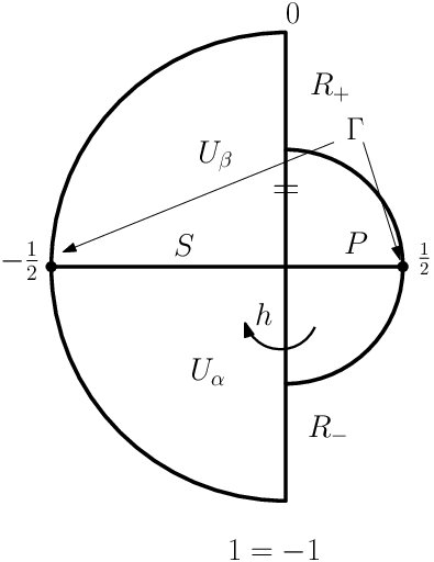
Every contact 3–manifold with convex boundary $(Y,\xi)$ admits a partial open book decomposition that is compatible with $\xi$ in the above sense, cf. [12]. To see this, consider a contact cell–decomposition for $Y$ whose 1–skeleton $C$ is a direct product near the boundary $\partial Y$ and intersects the boundary on the dividing set. As Legendrian arcs have standard neighbourhood, there is a neighbourhood $\nu(C)$ of $C$ with convex boundary and with dividing curves of two components. The dividing curve separates $-\partial\nu(C)$ into a positive and a negative part $(-\partial\nu(C))_{+}$ and $(-\partial\nu(C))_{-}$. Setting $P=(-\partial\nu(C))_{+}$ the neighbourhood $\nu(C)$ can be written as $P\times[0,1]/\sim$. As $C$ was the 1–skeleton of a contact cell–decomposition, $Y-\nu(C)$ is product disk–decomposable: it is divided by the 2–cells of the contact cell–decomposition (that are disks with $\mathrm{tb}=-1$) to a union of tight contact 3–balls. Thus for $S=\partial(Y-\nu(C))_{+}$ the handlebody $Y-\nu(C)$ can be written as $Y-\nu(C)=S\times[-1,0]/\sim$, and $P=(-\partial(\nu(C)))_{+}\subseteq(\partial(Y-\nu(C)))_{+}=S$. Note that by construction $\xi|_{Y-\nu(C)}$ is tight, its boundary $\partial(Y-\nu(C))$ is convex, and the dividing set $\Gamma_{\partial(Y-\nu(C))}$ is isotopic to $\partial S\times\{0\}$.

Next we review the change of the partial open book decomposition after a bypass is attached along a Legendrian curve $c$ on the boundary. For a complete discussion of bypass attachments see [11]. The considerations below already appeared in [12, Example 5].

Let $(Y,\partial Y,\xi)$ be a contact 3–manifold with convex boundary. Suppose that we are given a Legendrian arc $c\subset\partial Y$ that starts and ends on the dividing set $\Gamma_{\partial Y}$ and intersects $\Gamma_{\partial Y}$ in one additional point. Attaching a bypass along $c$ is — roughly speaking — the attachment of the neighbourhood of a “half overtwisted disk”. This is a disk $D$ with boundary $\partial D=c\cup d$, where $\partial D\cap\partial Y=c$, and the dividing curve on $D$ consists of a single arc with both of its endpoints on $c$. The resulting manifold is diffeomorphic to $Y$ with contact structure $\xi^{c}$, and the dividing curve $\Gamma$ is changed in the neighbourhood of $c$ to $\Gamma^{c}$ as it is shown on Figure 3.

Take a partial open book decomposition for $(Y,\partial Y,\xi)$ coming from a contact cell–decomposition whose 1–skeleton $C$ misses the attaching arc $c$. Let $c_{\pm}=c\cap R_{\pm}$. Under the identification of $Y-\nu(C)$ with $S\times[-1,0]/\sim$ both $c_{+}$ and $c_{-}$ are arcs on $S$. The bypass attachment can be thought of consisting of a 1–handle attachment with core $d$ followed by a canceling 2–handle attached along the curve $a=a_{+}\cup a_{-}$ of Figure 4. The contact cell–decomposition can be extended to the new manifold $(Y^{\prime},\xi^{\prime})$ (where $Y^{\prime}$ is, in fact, diffeomorphic to $Y$) by including the cocore of the 2–handle in the 1–skeleton. Thus $C^{\prime}=C\cup(\textrm{cocore of the 2--handle})$ and the page $S^{\prime}$ of the partial open book decomposition resulting from this contact cell–decomposition will be equal to $S\cup(-\partial\nu(d))_{+}=S\cup(\textrm{1--handle})$. Denote the intersection of the attaching circle of the canceling 2–handle with the positive and negative parts of $\partial(Y\cup\{\textrm{1--handle}\})$ by $a_{\pm}=a\cap R^{\prime}_{\pm}$. As it is depicted in Figure 4, the arc $a_{+}$ can be pushed off to lie entirely in the boundary of the old manifold $Y$, thus $a_{+}\subset R_{+}$. Note that $c_{+}$ and $a_{+}$ are isotopic. They have one endpoint that agrees with the endpoint of both $c_{-}$ and $a_{-}$, and the other one is moved in the direction given on $\Gamma_{\partial Y}$ as the boundary of $R_{+}$. These curves can again be thought of as being on $S$. Now $R_{+}^{\prime}=(R_{+}-\nu(a_{+}))\cup(\partial(-\nu(d)))_{+}$, thus $P^{\prime}=P\cup\nu(a_{+})$. The mondoromy $h^{\prime}$ remains the same on $P$, so we only need to understand it on $a_{+}$. To push $a_{+}$ through $\nu(C)$ we just have to push it through the newly attached 1–handle, so $h^{\prime}(a_{+})=a_{-}$. The arc $a_{-}$ can be split to two subarcs $a_{-}\cap S$ and the core of the 1–handle in $S^{\prime}$.

We give a short description of basic slices defined by Honda [11]. Suppose that $\xi$ is a contact structure on $T^{2}\times[0,1]$ with convex boundary with two–component dividing curves on each of its boundary components. The dividing curves are homotopically nontrivial and parallel. Fix a trivialization for $T^{2}$ as $\mathbb{R}^{2}/\mathbb{Z}^{2}$ and let $s_{i}$ denote the slope of the dividing curves on $T^{2}\times\{i\}\$ ($i\in\{0,1\}$). The contact 3–manifold $(T^{2}\times[0,1],\xi)$ is called minimally twisting if every convex torus parallel to the boundary has slope $s$ in $[s_{1},s_{0}]$. (By $[s_{1},s_{0}]$ we mean $[s_{1},\infty]\cup[-\infty,s_{0}]$ if $s_{1}\geq s_{0}$.) A basic slice is a minimally twisting tight contact structure $(T^{2}\times[0,1],\xi)$, with convex boundary and with two dividing curves on each $T^{2}\times\{i\}$ and boundary slopes $s_{0}$ and $s_{1}$ forming an integral basis for $\mathbb{Z}^{2}$. For fixed boundary conditions (up to isotopy) there are two basic slices distinguished by their relative Euler class, which differ by their sign; there is no canonical positive or negative choice.

One way to obtain a basic slice is by gluing a bypass to an $I$–invariant neighbourhood of a convex $T^{2}$ with two dividing curves. For a given slope of the attaching curve there are two ways of attaching a bypass corresponding to the two different basic slices, cf. Figure  6. Any basic slice can be obtained by this construction.

Suppose that $(T^{2}\times[0,1],\xi_{0})$ and $(T^{2}\times[1,2],\xi_{1})$ are basic slices with boundary slopes $s_{i}$ on $T^{2}\times\{i\}\$ ($i\in\{0,1,2\}$). As the dividing curves match up on $T^{2}\times\{1\}$, we can glue them together to obtain $(T^{2}\times[0,2],\xi=\xi_{0}\cup\xi_{1})$. If in addition we require that the shortest representatives of $s_{0}$ and $s_{2}$ give an integral basis for $\mathbb{Z}^{2}$ and $[s_{0},s_{1}]\cup[s_{1},s_{2}]\neq[-\infty,\infty]$, then $(T^{2}\times[0,2],\xi)$ is minimally twisting. It is either overtwisted or a single basic slice depending on whether the basic slices $(T^{2}\times[0,1],\xi_{0})$ and $(T^{2}\times[1,2],\xi_{1})$ have the same or opposite signs. Note that “having the same sign” makes sense in this setting, once we require the trivialization of $\xi_{0}$ and $\xi_{1}$ to agree over $T^{2}\times\{1\}$.

Suppose that $(Y,\xi)$ is a contact 3–manifold with convex boundary, and consider a partial open book compatible with $\xi$. Let $\{b_{1},\dots,b_{k}\}$ be a basis for $H_{1}(P,\partial S\cap\partial P)$. The disks swept out by the $b_{i}$’s in the $U_{\beta}$ handlebody have boundaries $\beta_{i}=b_{i}\times\{\frac{1}{2}\}\cup b_{i}\times\{-\frac{1}{2}\}$. Isotope each $b_{i}$ to an arc $a_{i}$ that intersects it transversely in a single point, and whose endpoints are moved in the direction given by the boundary orientation of $-P$. In the $U_{\alpha}$ handlebody $a_{i}$ sweeps out a disk with boundary $\alpha_{i}=a_{i}\times\{\frac{1}{2}\}\cup h(a_{i})\times\{-\frac{1}{2}\}$, providing a Heegaard diagram $(\Sigma,\mbox{\boldmath$\alpha$},\mbox{\boldmath$\beta$})$ for $(Y,\Gamma)$. The single intersection point $\mathbf{y}=(a_{i}\cap b_{i})$ on $P\times\{\frac{1}{2}\}$ can be shown to represent a cycle in $\mathrm{SFC}(-\Sigma,\mbox{\boldmath$\alpha$},\mbox{\boldmath$\beta$})$, thus it defines an element $\mathrm{EH}(Y,\xi)$ in $\mathrm{SFH}(-Y,-\Gamma)$. (Notice the reversal of orientation of the Heegaard surface $\Sigma$.) As has been proven by Honda, Kazez and Matić [12], this element is independent of the choices made throughout its definition and gives the invariant $\mathrm{EH}(Y,\xi)$ of the contact structure $(Y,\xi)$. In the special case when the contact 3–manifold with convex boundary is given as the complement of a standard neighbourhood of a Legendrian knot in a closed contact 3–manifold $(Y,\xi)$, the resulting element will be denoted by $\mathrm{EH}(L)$. Note that by the Legendrian Neighbourhood Theorem, in this case $\Gamma$ consists of two parallel simple closed curves in $\partial(Y-\nu(L))$.

Consider an oriented, null–homologous Legendrian knot in the closed contact 3–manifold $(Y,\xi)$. There is an open book decomposition of $Y$ compatible with $\xi$ containing $L$ on one of its pages $S=S\times\{\frac{1}{2}\}$. Consider a properly embedded arc $b_{1}$ in $S$ intersecting $L$ exactly once. The disk $b_{1}\times[0,1]$ is a meridional disk for $L$. Orient $b_{1}$ so that the boundary orientation of $\partial(b_{1}\times[0,1])=-b_{1}\times\{0\}\cup b_{1}\times\{1\}$ agrees with the natural orientation of the meridian for $L$. (Such an oriented arc $b_{1}$ will be called a half–meridian of $L$.) With these conventions the orientation of $S$ coincides with the orientation induced by $(b_{1},L)$. Our setup here will be slightly different from the one used in [15], but the resulting Heegaard diagram and the element specified in it will be actually the same already on the chain–level.

Pick a basis $\{b_{1},\dots,b_{g}\}$ of $H_{1}(S,\partial S)$ such that $b_{1}$ is a half–meridian of $L$. Isotope all the $b_{i}$’s to $a_{i}$’s as before and place the basepoint $z$ in the “big” region that is not swept out by the isotopies of the $b_{i}$, and put $w$ between $b_{1}$ and $a_{1}$. This can be done in two essentially different ways, and exactly one of them corresponds to the chosen orientation of $L$. If $b_{1}$ is oriented as described above, $w$ should be placed close to the tail of $b_{1}$, cf. Figure 5.

The single intersection point $(a_{i}\cap b_{i})$ on $S\times\{\frac{1}{2}\}\subset-\Sigma$ is an element in $\widehat{\mathrm{CFK}}(-\Sigma,\mbox{\boldmath$\alpha$},\mbox{\boldmath$\beta$},z,w)$ and the choice of $z$ assures that it is a cycle, hence it defines an element $\widehat{\mathcal{L}}(L)$ in $\widehat{\mathrm{HFK}}(-Y,L)$. As it was shown in [15], the homology class $\widehat{\mathcal{L}}(L)$ is an invariant of the oriented Legendrian knot $L\subset(Y,\xi)$.

References

- [1] Y. Chekanov, Differential algebra of Legendrian links, Invent. Math. 150 (2002), 226–483.
- [2] Y. Eliashberg, Invariants in contact topology, in Proceedings of the International Congress of Mathematicians, Vol II (Berlin, 1998), Doc. Math. 1998, Extra Vol. II, 327–338.
- [3] Y. Eliashberg and M. Fraser, Topologically trivial Legendrian knots, arXiv:0801.2553. (also Classification of topologically trivial Legendrian knots, in Geometry, topology, and dynamics (Montreal, PQ, 1995), 17–51, CRM Proc. Lecture Notes 15, Amer. Math. Soc., Providence, RI, 1998.)
- [4] T. Etgü and B. Ozbagci, Partial open book decompositions and the contact class in sutured Floer homology, arXiv:0711.0880.
- [5] T. Etgü and B. Ozbagci, Relative Giroux correspondence, arXiv:0802.0810.
- [6] J. Etnyre, Legendrian and transversal knots, In Handbook of knot theory, pages 105–185. Elsevier B. V., 2005.
- [7] J. Etnyre, Private communication.
- [8] J. Etnyre and K. Honda, Knots and contact geometry. I. Torus knots and the figure eight knot, J. Symplectic Geom. 1 (2001), 63–120.
- [9] P. Ghiggini and K. Honda, Giroux torsion and twisted coefficients, arXiv:0804.1568.
- [10] P. Ghiggini, K. Honda and J. Van Horn-Morris, The vanishing of the contact invariant in the presence of torsion, arXiv:0706.1602.
- [11] K. Honda, On the classification of tight contact structures I., Geom. Topol. 4 (2000), 309–368.
- [12] K. Honda, W. Kazez and G. Matić, The contact invariant in sutured Floer homology, arXiv:0705.2828.
- [13] K. Honda, W. Kazez and G. Matić, Contact structures, sutured Floer homology and TQFT, arXiv:0807.2431.
- [14] A. Juhász, Holomorphic discs and sutured manifolds, Algebr. Geom. Topol. 6 (2006), 1426–1457.
- [15] P. Lisca, P. Ozsváth, A. Stipsicz and Z. Szabó, Heegaard Floer invariants of Legendrian knots in contact 3-manifolds, arXiv:0802.0628.
- [16] L. Ng, P. Ozsváth and D. Thurston, Transverse knots distinguished by knot Floer homology, arXiv:math/0703446.
- [17] B. Ozbagci and A. Stipsicz, Surgery on Contact 3-Manifolds and Stein Surfaces, Bolyai Society Mathematical Studies, Vol. 13, Springer-Verlag, Berlin, 2004.
- [18] P. Ozsváth and A. Stipsicz, Contact surgeries and the transverse invariant in knot Floer homology, arXiv:0803.1252.
- [19] P. Ozsváth and Z. Szabó, Holomorphic disks and topological invariants for closed three-manifolds, Ann. of Math. 159 (2004), 1027–1158.
- [20] P. Ozsváth and Z. Szabó, Holomorphic disks and three-manifold invariants: properties and applications, Ann. of Math. 159 (2004), 1159–1245.
- [21] P. Ozsváth and Z. Szabó, Holomorphic disks and knot invariants, Adv. Math. 186 (2004), 58–116.
- [22] P. Ozsváth, Z. Szabó and D. Thurston, Legendrian knots, transverse knots and combinatorial Floer homology, Geom. Topol. 12 (2008), 941–980.
- [23] J. Rasmussen, Floer homology and knot complements, Phd thesis, Harvard University, 2003, math/0607691.
- [24] I. Torisu, Convex contact structures and fibered links in 3-manifolds, Internat. Math. Res. Notices 9 (2000), 441–454.
- [25] D. S. Vela–Vick, On the transverse invariant for bindings of open books, arXiv:0806.1729.