MPP-2008-53
Squark–anti-squark pair production at the LHC:
the electroweak contribution
W. Hollik and E. Mirabella
Max-Planck-Institut für Physik
(Werner-Heisenberg-Institut)
Föhringer Ring 6,
D-80805 München, Germany
Abstract
We present the complete NLO electroweak contribution of to the production of diagonal squark–anti-squark pairs in proton–proton collisions. Compared to the lowest-order electroweak terms, the NLO contributions are also significant. We discuss the LO and NLO electroweak effects in cross sections and distributions at the LHC for the production of squarks different from top squarks, in various supersymmetric benchmark scenarios. LO and NLO can add up to in cross sections and in distributions.
1 Introduction
The exploration of electroweak symmetry breaking will be one of the main
tasks at the Large Hadron Collider (LHC). Experiments are expected to either
verify the Higgs mechanism of the Standard Model (SM), or to detect signals
of physics beyond the SM. The concept of supersymmetry [1, 2] provides a
promising alternative version of the Higgs mechanism where symmetry breaking
occurs without introducing new scalar couplings that potentially can
become strong,
thus stabilizing the electroweak scale.
The realization of supersymmetry in terms of
the Minimal Supersymmetric Standard Model (MSSM) [3, 4, 5],
has come up as the most promising extension of the SM,
a predictive framework that allows to make
precise predictions to be investigated
by indirect and direct experimental studies.
The indirect access through virtual effects in
electroweak precision data [6]
provides an overall fit [7, 8]
with a quality at least as good as in the SM, in specific observables
like of the muon [9, 10] even better,
and yields bounds on the
light Higgs boson mass with less tension than in the SM [11, 12, 13].
If supersymmetry (SUSY) is realized at the TeV scale or below,
it will be accessible to
direct experimental studies at the LHC through the production of SUSY
particles.
In particular, colored particles like squarks and gluinos
will be copiously produced, and the hadronic production of
squark– anti-squark pairs is expected to play an important role
for SUSY hunting.
The cross section is in the range from
pb for masses of squarks and gluinos below 1 TeV
and can be measured with a statistical uncertainty
of the order of a few percent even in the low luminosity regime.
Moreover, squark cascade decays into
lead to a signature with missing plus jets and possibly leptons
that is well suited to detect MSSM signals [14, 15].
The number of hard jets allows the distinction
between gluino and squark decays. Finally with the help of
decay chains one can reconstruct the mass of the squarks up to 2 TeV
with a resolution better than [16, 17, 18].
The first prediction of the
cross section for hadronic production of squark pairs
in the early 1980’s was done at lowest order
in supersymmetric QCD [19, 20, 21, 22, 23].
QCD contributions at NLO,
, for the processes
were calculated more than ten years later [24, 25].
They increase the cross section by
typically , and they
substantially reduce the dependence on the factorization
and renormalization scale.
NLO QCD corrections to the production of top-squark pairs,
performed in [26], are also positive
and can increase the cross section by 40–50%.
Besides the QCD-based production mechanisms,
there are also partonic processes of electroweak
origin, like diagonal and non-diagonal
squark pair production from annihilation [27, 28].
They proceed
through -channel photon and exchange, and also through
neutralino/chargino exchange in the -channel (if
is different from ), yielding terms of
and .
Due to interference between the tree-level QCD
and electroweak amplitudes for ,
the electroweak contributions can also become sizable,
reaching values up to 20% [27].
For reliable predictions, electroweak contributions at NLO have to be taken into account as well. In the case of top-squark pair production [29, 30, 31], they were found to be significant, with effects up to 20%. In general, NLO electroweak (EW) contributions consist of loop contributions to the tree-level amplitudes for annihilation and gluon fusion, together with real photon and gluon bremsstrahlung processes, yielding an involved struture of interference terms in annihilation. Moreover, photon–gluon induced parton processes also contribute owing to the non-zero photon distribution in the proton. In this paper we present the NLO electroweak contributions, of , to the production of diagonal squark–anti-squark pairs different from top- and bottom-squarks,
| (1) |
They show significant differences to top-squark production, based on the following pecularities.
- •
In leading order , the squark pair can be produced via annhilation of a pair through amplitudes that involve also the exchange of a gluino in the -channel, thus enhancing the relative weight of the annihilation channel in (1).
- •
Electroweak tree diagrams with -channel neutralino and chargino exchange are part of the amplitudes for and , where is the isospin partner of in a quark doublet, yielding EW–QCD interference already at the tree-level.
- •
At many types of interferences occur between amplitudes of and as well as between and amplitudes.
These features make the calculation of the EW contributions
of
to the processes (1)
more involved than in the case of production
where no -channel diagrams occur at lowest order.
Our analysis shows that the EW effects of NLO
can reach the same size as the tree-level EW contributions of
and , which we will
include in our discussion as well.
The case of production will not be treated here.
Owing to -tagging, bottom-squarks can
be experimentally distinguished from the squarks of the first two
generations [18, 32, 33]. Moreover, in the case of production the partonic process exhibits specific features, like
mixing between left- and right-handed -squarks,
mixing angle renormalization [34], non-negligible
Higgs-boson contributions and
enhanced Yukawa couplings for large vaues of with the need of
resummation [35];
other peculiarities for massive initial-state partons
are the proper counting of the orders of the perturbative
expansion [36, 37] and the
appropriate choice of the factorization scale [38].
A dedicated extra analysis for -squark final states thus seems
appropriate.
The outline of the paper is as follows. In Section 2 we briefly summarize the various tree-level contributions to the processes (1). Section 3 describes the structure of the NLO terms of EW origin that contribute at and the strategy of the calculation. Evaluation of the EW effects and their analysis for the LHC are presented in Section 4 and summarized in Section 5. A list of Feynman diagrams and counter terms with specification of renormalization, and technical details for the calculation of singular integrals are collected in the Appendix.
2 Tree-level contributions to squark pair production
In this section we list the lowest-order cross sections for the process (1) arising from tree-level amplitudes at order , and . We will use the convention to denote the cross section for a partonic process at a given order in the strong and electroweak coupling constants. The parton luminosities for getting to the hadronic cross section are given by the convolution
| (2) |
where is the momentum distribution of the parton in the proton (PDF).
2.1 Squark pair production at leading order
The leading-order contribution to the process (1) is QCD based, of . In the notation mentioned above, the differential cross section reads as follows,
| (3) |
The sum runs over the quarks . S and are the squared CM energies of the hadronic process (1) and of the partonic subprocess, respectively. Moreover, with the squark mass , the threshold value is determined by .
and denote the differential cross sections for the partonic processes
| (4) | |||||
| (5) |
respectively, which are obtained from the Feynman diagrams in Fig. 4 of Appendix A. Explicit expressions for these leading-order cross sections can be found in Refs. [19, 22, 23]. Owing to flavour conservation in SUSY QCD, the diagram with the exchange of a gluino in the channel contributes only if .
2.2 Tree-level electroweak contributions of and
The and contributions to the process (1), involving electroweak terms, can be written as follows,
| (6) |
The parton cross section
is obtained squaring the tree-level
electroweak diagrams depicted in Fig. 4 of Appendix A.
The diagram with -channel neutralino exchange contributes only if , and
the diagram with chargino exchange appears only if ,
being the SU(2) partner of the quark , since we
treat the CKM matrix as unity.
originates from interference between the aforementioned
tree-level electroweak diagrams and the tree-level QCD graphs of Fig. 4.
Analytical expressions for
these cross sections can be found in Ref. [27].
As a new element at , photon–gluon fusion occurs as a further partonic process,
| (7) |
The corresponding cross section, with ,
| (8) |
contains the spin- and color-averaged squared tree-amplitudes from the diagrams in Fig. 4,
with , and the electric charge of the squark . The presence of photons in the proton follows from including NLO QED effects in the evolution equations for the PDFs. The photon PDF is part of the publicly available PDF set of [39]; together with the gluon PDF, the luminosity entering (6) is built according to Eq. (2).
3 Virtual and real corrections
In this section we describe the computation of the corrections to the process (1) arising from loops and from photon/gluon bresmsstrahlung. The corresponding contributions to the hadronic cross section are expressed in obvious notation,
| (9) | |||||
Other bremsstrahlung contributions to the hadronic cross section are of the type
| (10) |
We will not consider this class of processes here; they are further
suppressed by an additional factor with
respect to process (7), and thus negligible.
Diagrams and corresponding amplitudes are generated using
FeynArts [40, 41]. The algebraic treatment and numerical evaluation
of loop integrals is performed with support of FormCalc and LoopTools [42, 43].
IR singularities are regularized by a small photon mass, while quark masses
are kept as regulators for the collinear singularities.
3.1 Gluon fusion with electroweak loops
The first class of corrections entering Eq. (9) are the electroweak virtual contributions to fusion (5), given by the partonic cross section
| (11) |
is the tree level amplitude (Fig. 4), and
is the one-loop amplitude with EW insertions in the QCD-based tree diagrams.
These loop diagrams
do not depend on the flavour of the final squark and thus they are identical to those listed in [30]
for the particular case of .
We therefore do not repeat them here.
In order to get rid of the UV divergences we have to include the proper counterterms for one-loop renormalization.
Their explicit expressions in terms of
the renormalization constants can be found in Appendix B.
In the case of the gluon-fusion subprocess we have to
renormalize the squark sector only.
We use the on-shell scheme [30, 44, 34], where the independent parameters
for a squark isospin doublet11
1
Due to SU(2) invariance, mass renormalization
of the different squarks from the same SU(2) doublet is correlated
and has to be performed simultaneously.
are chosen
to be the masses of the two up-squarks, the mass of one of the two down-squarks,
and the two mixing angles (which, however are irrelevant for the light-quark squarks where mixing can be neglected).
The actual expressions for the renormalization constants are also given
in Appendix B.
Notice that part of the virtual corrections to squark pair production are loop diagrams for the gluon-gluon- vertex, with the heavy neutral MSSM Higgs boson . These terms become resonant when and have to be considered a contribution to the process of production via gluon fusion with the subsequent decay , rather than an electroweak loop correction. We will not consider scenarios in which such resonances occur.
3.2 Gluon fusion with real photon emission
The IR singularities arising from virtual photons in (11) are cancelled by including bremsstrahlung of real photons at ,
| (12) |
according to the diagrams depicted in Fig. 4.
The integral over the photon phase space is IR divergent in the soft-photon region,
i.e. for , and cancels the corresponding virtual singularities
when added to the virtual contributions according to Eq. (9).
For the technical treatment of photon-momentum integration and isolation of divergences
we apply two different procedures: the methods of dipole subtraction
and of phase space slicing.
In the dipole subtraction approach, one has to add and subtract
an auxiliary function to the differential cross section
that matches pointwise the singuilarities
and is easy enough to be integrated analytically; the integral over the subtracted cross section is
convergent and can be done numerically.
Due to the universality of the soft singularities general expression for these functions are available.
In particular we use
the expressions given in Ref. [45]. Although the formulae
quoted in this reference apply to processes
involving fermions only,
they can be generalized to processes with charged bosons owing to the
universal structure of the IR singularities.
The phase space slicing technique restricts the phase space integration to the region with a minimum photon energy . The integration over this region is thus convergent and can be performed numerically. The complementary integral over the singular region with can be done analytically in the eikonal approximation [46], which is a good approximation if the cut is sufficiently small. More details are given in Appendix C. Comparison between the two methods provides a non trivial check of the computation. As illustrated in Fig. 12, the two methods yield results which are in good numerical agreement.
3.3 annihilation with electroweak and QCD loops
The structure of the parton processes of annihilation at higher order is more involved and requires a simultaneous treatment of electroweak and QCD loops. The virtual contributions of one-loop order to the partonic cross section is given by the interference of tree-level and loop amplitudes,
| (13) |
where () is the amplitude related to the tree-level QCD (EW) diagrams
depicted in Fig. 4 (4). is the one-loop amplitude arising from the
EW corrections to the QCD tree-level diagrams and the QCD corrections to the EW tree-level diagrams.
Finally, is the one-loop amplitude corresponding
to the QCD corrections to the QCD tree-level diagrams.
The diagrams entering are displayed in
Figs. 5–7
of Appendix A.
They also contain the diagrams with counterterm insertions required for renormalization and cancellation
of UV divergences.
The counterterms and the necessary renormalization constants can be found in Appendix B.
Besides squark renormalization, also quark renormalization is needed.
can be obtained from the Feynman diagrams in Fig. 8 of Appendix A, including the proper counterterms. Besides renormalization of the squark sector, we have to renormalize also the gluino mass, the strong coupling , and the quark–squark–gluino coupling , which is related to via supersymmetry. The strong coupling constant is renormalized in the scheme, modified according to Ref. [24] in order to decouple heavy particles (top, gluino, squarks) from the running of . For the non-standard loop contributions, this procedure is equivalent to the “zero-momentum subtraction” used in Ref. [47]. Since dimensional regularization violates supersymmetry in higher orders, a finite difference between and is encountered at one-loop order. Supersymmetry is restored by shifting the renormalization constant for by the corresponding finite amount, which means an unsymmetric renormalization of and . More details and the specification of the counterterms can be found in Appendix B.
3.4 annihilation with real photon emission
The diagrams in Fig. 9 of Appendix A constitute the generic amplitude for photon bremsstrahlung at in the annihilation channel,
| (14) |
The corresponding cross section is singular both in the IR soft-photon region and in the collinear region (e.g. whenever ). Although IR singularities cancel in sufficiently inclusive observables, collinear singularities from initial-state radiation remain and have to be absorbed via factorization in the PDFs.
The extraction of the singularities has been performed using the two different methods described in section 3.2. In phase space slicing, in this case, we have to introduce a further collinear cutoff on the angle between the photon and the radiating quark/antiquark. For sufficiently small , the integral over the singular region can be performed analytically. Explicit expressions can be found in Appendix C. In Fig. 12 we visualize the comparison between the two methods in the specific case of the partonic process as an example.
3.5 annihilation with real gluon emission
Finally, we have to take into account the class of annihilation processes with real gluon bremsstrahlung,
| (15) |
from either EW-based (Fig. 10 a) or QCD-based Born diagrams (Fig. 10 b). This class contributes to the cross section at through interference between the graphs of Fig. 10 a and Fig. 10 b. The cross section exhibits singularities when the gluon becomes soft or collinear to the initial-state quark/antiquark. The soft singularities cancel against those from the virtual photon/gluon contributions in annihilation, when added along Eq. (9), while remaining collinear singularities have to be absorbed in the PDFs by factorization. IR and collinear singularities can be treated by mass regularization.
For applying the phase space slicing method, the eikonal current has to be modified due to colour correlations after the emission of the soft gluon (see Refs. [48, 49, 50] and Appendix C for details). Colour correlation has to be taken into account also when using the Dipole Subtraction Method; we modified the formulae of Ref. [45] accordingly, following the guidelines of Ref. [48]. In Fig. 12 we illustrate the comparison between the two methods also for gluon radiation, with good numerical agreement.
3.6 fusion
A last class of partonic processes at the considered order is given by (anti-)quark-gluon fusion,
| (16) |
This IR finite class contributes at through the interference between the diagrams of Fig. 11 a and Fig. 11 b. Mass singularities arise when the incoming gluon and outgoing (anti-)quark are collinear. These collinear divergences are again absorbed into the PDFs. Their extraction has been performed using the two methods described above in section 3.2. Explicit expressions for the cross section in the collinear region can be found in Appendix C. The actual expression of the subtraction function used in the Dipole Subtraction method is obtained from the formulae in Ref. [51]. Since those formulae are given there for the case of photon–quark splitting we have to consistently redo the color algebra. In Fig. 12 we show the agreement between the two methods for the example .
In specific cases of SUSY parameters, when kinematically allowed, the internal-state gauginos can be on-shell. The poles are regularized by introducing the width of the corresponding gluino, neutralino, or chargino. Potential problems related to gauge invariance [52] do not occur here.
3.7 Factorization of initial-state collinear singularities
The corrections to partonic cross sections contain universal initial-state collinear singularities that can be absorbed into the PDFs choosing a factorization scheme where singularities of relative order , the lowest order PDF for parton ) is related to the experimentally accessible distribution via [53, 54]
| (17) | |||||
with the factorization scale , , and the electric charge . The splitting functions , are defined in the usual way,
| (18) |
and the functions and are given by
| (19) |
The actual effect of the factorization of the initial collinear singularities is to substitute by in the definition of the quark–antiquark luminosity (2) and thus to obtain a further contribution to be added to Eq. (9). This contribution reads:
| (20) |
where , while and are defined as
| (21) | |||||
The singularities in cancel in the sum of the real
corrections and of the contribution (20), as can be easily checked using the analytic
expressions of and in the collinear regions [see Eqs. (39)
and (43) of Appendix C]. The remaining singularities of the real corrections
are exactly cancelled against those in and in
the virtual corrections.
The mass singularities in the last line of Eq. (20) are
cancelled by those of
and
, as
can be inferred from the their analytic expressions in the collinear region
[Eq. (44) of Appendix C].
| parameter | SPS1a′ | SPS5 | SU1 | SU4 |
|---|---|---|---|---|
| GeV | GeV | GeV | GeV | |
| GeV | GeV | GeV | GeV | |
| GeV | GeV | GeV | ||
For the calculation of hadronic observables we use the MRST2004qed parton distribution functions [39]. Factorization and renormalization scales are chosen as equal, .
4 Numerical Analysis
For the numerical evaluation and for illustration of the EW effects, we choose
four different benchmark scenarios: the point SPS1a′ suggested by the SPA convention [55], the snowmass point
SPS5 [56] characterized by light stops,
and two of the points chosen for detector simulation in the ATLAS “Computing System Commissioning”
exercise [57]: the point SU1 in the coannihilation region, and the
point SU4 characterized by light SUSY particles. The input parameters
, , , defined at the GUT scale, and
are put together in Table 1.
The MSSM input for the actual calculation is obtained with the help of
the program SPheno [58], together with
the program SuSpect [59] as a cross check.
The pole masses of the squarks of the first generation obtained with the two different codes are shown
in Table 2. Since the quarks of the first two
generations are treated as massless, same-chirality and same-isospin
squarks are degenerate, therefore we do not show the masses of the
squarks belonging to the second generation.
The difference between the masses provided by the two
codes is below . The different inputs given by the two codes
give rise to a differences in the total cross section of the
order of . The standard model parameters are taken from
Ref. [60].
| SPS1a′ | SPS5 | SU1 | SU4 | |
|---|---|---|---|---|
| () | () | () | () | |
| () | () | () | () | |
| () | () | () | () | |
| () | () | () | () |
We introduce the following conventions:
- •
We will refer to the sum of , and contributions as “the EW contribution”.
- •
We will use the quantity to denote the relative EW contribution, defined as , where is a generic observable and is the sum of the LO in Eq. (3) and the EW contribution.
4.1 Different squark species
Electroweak interactions depend on the hypercharge of the squarks, hence the production cross sections are flavour
and chirality dependent.
In this subsection we will study the production of
four squark species, focusing on the SPS1a′ point.
Since the masses of the light quarks can be neglected,
the weak eigenstates of the squarks are also the mass eigenstates;
thus, in the following, the two squarks of a given flavour are distinguished
by means of their chiralities, .
Dependence on squark flavour and chirality
In Tab. 3 we show the integrated hadronic cross section for the diagonal pair production of , , and . In the case of the production of the squarks of the first generation there is a cancellation beetween and contributions. The overall correction is negative and of the same order of magnitude as the one. Since they have the same sign their effect is enhanced. In the case of production the situation is different: , , and corrections are positive, contribution being the most important ones (see also the discussion below).
As a general remark, the EW effects are always larger for left-handed squarks.
For a given chirality and generation, the EW contributions are more important in
in the case of up-type squarks. For comparison we
also estimate the corresponding NLO QCD corrections using the code PROSPINO [25];
they are positive, weakly dependent on the flavour of the produced squarks, and of the order of .
Fig. 13 shows the relative EW contribution (right part) in
the “cumulative invariant mass distribution” , that is the cross section integrated up to
the value of the squark–antisquark invariant mass. A common feature is that in the low invariant mass region the NLO EW contribution
is positive, rather steeply decreasing as the invariant mass increases, reaching the plateau at GeV
which corresponds to the total cross section. The left part of Fig. 13
shows the relative size of the individual contributions arising from the various channels.
The contribution from the gluon fusion channel is always positive and dominates at lower values of , wheras the
annihilation channel part is negative.
Looking at the relative contributions of the different channels in the
high invariant mass region, which corresponds to the total cross section, one can
understand the origin of the different behaviour of the NLO EW
corrections in the case of and production.
For up-squark pairs, the and terms are dominated by the
the annihilation channels, which yield a negative contribution;
for charm-squark production, however, the
[]
corrections are dominated by
the fusion [ fusion] channel and thus positive
This shows
the key role played by the partonic processes
,
where and belong to the same isospin doublet.
Indeed, in the case of production their
contribution is negative and the largest out of the
annihilation channels.
In production they are suppressed by the PDFs
of the charm and strange quarks and hence the
contributions from the annihilation channels
are negligible. As a result the overall contribution to
total cross section is
negative at the level of 5% for the left-handed up-squarks, while for
the left-handed charm-squarks it is of the same order of magnitude but
positive.
The contribution of the channel is independent on the squark chirality, determined
only by the electric charge of the produced squarks, which makes
the channel contribution
for up-squark pair production four times bigger than that for
down-squarks. Owing to the mass degeneracy between same-chirality and
same-isospin squarks the fusion
channel is independent on the generation of the produced squark.
The invariant mass distribution itself is displayed in Fig. 14 for the various squark species, showing also the breakdown
into the individual channels.
For each squark species, the EW contributions are positive in the low invariant mass region
and become negative for larger values of , reaching the level of 15% for squarks.
Fig. 15 contains
the transverse momentum distribution of the squarks.
Again, the EW effects are more pronounced for left-handed chirality
yielding more than 30% negative contributions for large . As new feature, the LO EW contribution can be positive for low ,
especially for the case, originating from the PDF-enhanced parton process
through -channel chargino exchange. This positive part is practically compensated by the NLO
contributions in the annihilation channel.
Dependence on the squark masses
To study the dependence of the NLO EW contributions on the mass of the squarks,
we vary , setting
and with , which is the
value at the SPS1a′ point. The values are also taken for the other generations as well as
for the sleptons. The other parameters are kept as in SPS1a′.
Each parameter point was checked to satisfy the bounds on SUSY particles from LEP [61, 62] and
Tevatron [63], and the bound on the mass of the
light Higgs boson , which has been computed using FeynHiggs 2.5.1 [64, 65, 66].
Moreover, each point fullfills the condition
,
where is the dominant squark contribution to the electroweak parameter.
The relative EW contributions are shown in Fig. 16 for the total cross section, for each of the various squark types. The quantity displayed in the right panel is the fraction of each the fusion and the annihilation channel in the total cross section, at leading order . The channel becomes more and more important as increases. This feature, already pointed out in Ref. [19], is a consequence of the -channel gluino exchange diagrams. The increasing importance of annihilation allows a better understanding of the particular role of the NLO corrections to the channel with increasing squark masses. Especially for left-handed up- and down-squarks, the NLO EW contributions become more important than the LO ones, with effects of more than 20%. In the charm-squark production case channel is subleading with respect to the and fusion channels due to the aforementioned suppression of charm and strange PDFs. The total sum of the EW contributions is shown in the right panel of Fig. 16. For illustration, we also give an estimate of the formal statistical uncertainty , assuming a luminosity .
4.2 Different SUSY scenarios
Here we discuss the electroweak effects
in the different SUSY scenarios mentioned above.
As a concrete example, we consider the production of squarks,
with the corresponding masses listed in
Table 2.
In Table 4 we show the total cross section for the
aforementioned production process. The LO contribution
and the different orders entering the NLO EW corrections are shown
separately. As one can see the absolute value of the different contributions
decreases as the mass of increases, while the
relative yield of the NLO EW corrections increases with the mass of
the produced squarks. In the case of the SU1 scenario NLO EW
corrections are negative and of the order of 10%. The corresponding
NLO QCD corrections
are estimated using the code PROSPINO [25];
they are of the order of .
| SPS5 | SU1 | SU4 | |
|---|---|---|---|
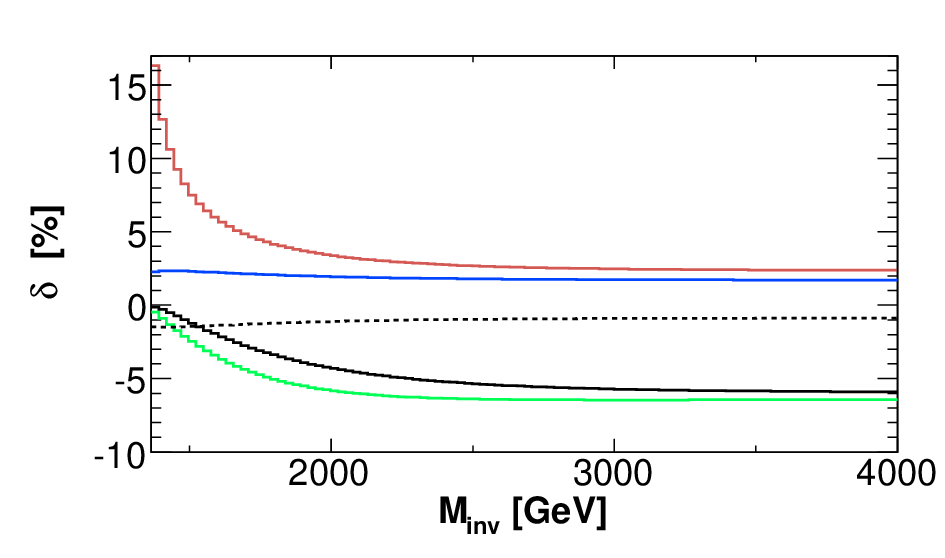
Fig. 17 contains the cumulative invariant mass distribution, again with the individual
and the total EW contributions, which show a similar behaviour for all the chosen scenarios.
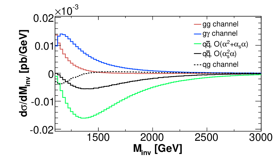
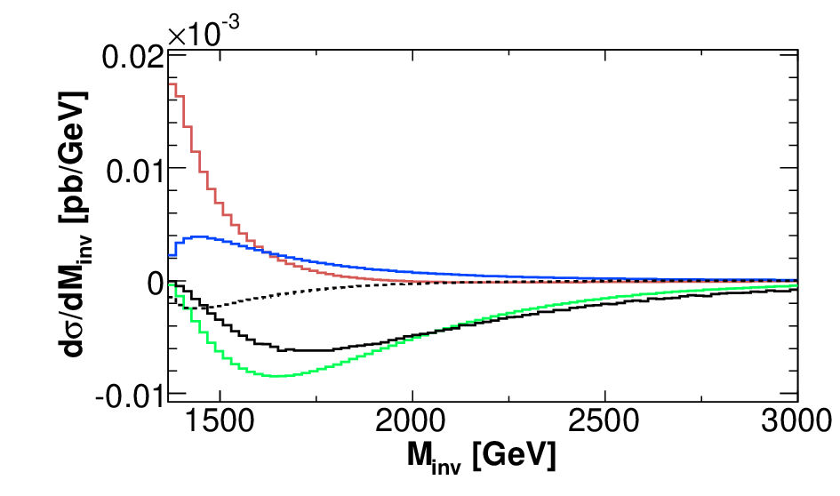
Also the differential invariant mass distribution, displayed in Fig. 18, has similar
qualitative features in all scenarios. At low values, the gluon fusion part dominates and
renders the total EW contribution positive. At larger values, the contributions from annihilation
turn the EW contribution to the negative region; thereby the NLO part is always of about the same size
as the LO part.
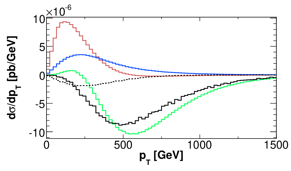
In Fig. 19 we show the transverse momentum distribution in the various cases. Again,
their shape depends only weakly on the scenario.
This general situation is only slightly changed when kinematical cuts are imposed, as we find from repeating our analysis for an exemplary set of cuts on the transverse momentum and on the rapidity of the two squarks,
The cut on the rapidity is not effective because the NLO EW contributions to the rapidity distribution are
very small
for . More important is the cut on the transverse momentum. It excludes the kinematical region where the largest part of the gluon channel
contribution comes from.
Moreover, this cut suppresses also the contribution of the channel and enhances the influence of the
channel by
excluding the region with a positive distribution.
As a result, the negative EW contribution to the total cross section is larger than without cuts, as one can see
from Fig. 20.
Dependence on the gluino mass
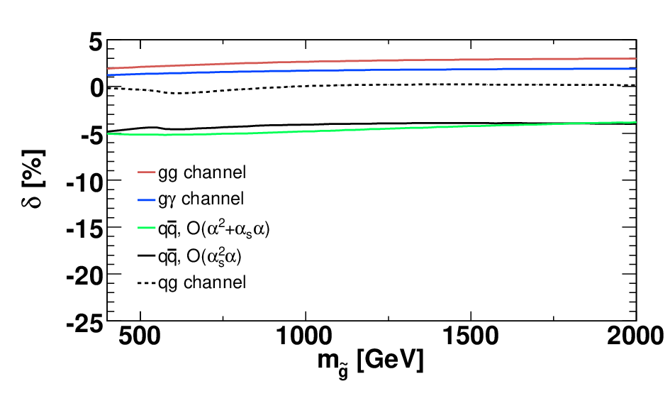
Finally we study the dependence of the EW contribution as a function of the mass of the gluino , with the other parameters kept fixed according to the SPS1a′ point. Again, the parameter range is in accordance with the phenomenological constraints described in the previous subsection 4.1. At LO, the gluon fusion channel does not depend on the gluino mass, while the annihilation channel contribution decreases with increasing , as displayed in Fig. 21. In the low region the two channel contribute equally to the production cross section, while gluon fusion becomes dominant as the mass of the gluino increases. The relative EW contributions from the various channels are flat, adding up to a total EW contribution from for gluino masses between 500 and 2000 GeV. Thereby, in annihilation, both the tree-level term and the NLO corrections , are practically of the same size.
5 Conclusions
We have computed the NLO electroweak contributions
to the production of flavour-diagonal squark–anti-squark pairs in proton–proton collisions,
in combination with the electroweak LO tree-level contributions of .
We have performed an explicit study of the electroweak contributions for
each case of the four squark species in the first SU(2) doublet,
with a numerical analysis for the LHC.
The electroweak effects can give rise to sizeable modifications in cross sections and distributions,
in particular for left-handed squarks.
Thereby, the NLO terms are significant and
have to be considered together with the tree-level contributions.
They show a strong dependence on the squark masses, increasing
their relative influence with the mass of the squarks.
Moreover, we have investigated several SUSY benchmark scenarios and found that the behaviour of the electroweak contributions is only weakly dependent on the scenario. Also the gluino-mass dependence is weak. In summary, the electroweak contributions in squark-pair production can reach 20–25% in size and are thus significant; about half is carried by the NLO contributions. As a final remark we would like to mention that the NNLO QCD contributions, of , can be expected to be of similar size.
Acknowledgments
We thank Stefan Dittmaier and Stefano Pozzorini for useful discussions, and Maike Trenkel for cross checking part of the results.
Appendix
Appendix A Feynman diagrams
In this Appendix generic diagrams for the various contributions to the different channels are shown. We choose the up-squark case as a specific example. In the following we will use the label () to denote all the neutral (charged) Higgs bosons, while .
(a)
(b)
(a)
(b)
Appendix B Counter terms and renormalization constants
Here we list the counter terms for renormalization of vertices and propagators in the one-loop amplitudes for squark-pair production. For squarks of the first two generations, we can neglect - mixing, and weak eigenstates are also mass eigenstates that can be distinguished by their chiralities . The Feynman rules for the counter terms can be expressed in terms of the field renormalization constants of quarks, squarks, gluons, and gluinos, defined from the relation between bare and renormalized fields,
| (22) |
together with the renormalization constants for the strong coupling , for the strong Yukawa coupling , and for the squark masses, which are defined according to
| (23) |
The actual expressions of the counterterms that are relevant for our squark-pair production processes are given below.
- •
Vertex counter terms involving gauge bosons:
![[Uncaptioned image]](0806.1433v2/SqSqGlCTT.png) =
=
![[Uncaptioned image]](0806.1433v2/Sq2Gl2CTT.png) =
=
![[Uncaptioned image]](0806.1433v2/QuQuGlCTT.png) =
=
![[Uncaptioned image]](0806.1433v2/QuQuZeCTT.png) =
=
![[Uncaptioned image]](0806.1433v2/SqSqZeCTT.png) =
=
and are the momenta of the squark and the antisquark, and they are fixed according to the arrow. are the color matrices and the structure constants of the color group. We omit the color indices of fermions and sfermions. Moreover, we define(24) where and are sine and cosine of the electroweak mixing angle .
- •
Self energy counter terms:
![[Uncaptioned image]](0806.1433v2/SqSqCTT.png) =
=
![[Uncaptioned image]](0806.1433v2/Gluino3CTT.png) =
=
![[Uncaptioned image]](0806.1433v2/GluGluCTT.png) =
=
- •
Vertex counter terms involving gauginos:
![[Uncaptioned image]](0806.1433v2/Gluino1CTT.png) =
=
![[Uncaptioned image]](0806.1433v2/Gluino2CTT.png) =
=
![[Uncaptioned image]](0806.1433v2/Neut1CTT.png) =
=
![[Uncaptioned image]](0806.1433v2/Neut2CTT.png) =
=
![[Uncaptioned image]](0806.1433v2/Cha1CTT.png) =
=
![[Uncaptioned image]](0806.1433v2/Cha2CTT.png) =
=
The Feynman rules involving Majorana particles follow the prescription of Ref. [67]; in particular the fermion flow is fixed according to the arrow depicted in the quark line. As usual, denotes the SU(2) partner of . The vertices involving neutralinos contain the quantities(25) where is the mixing matrix of the neutralinos. can be expressed in terms of the mixing matrices and of the chargino sector: for up [down] type quarks.
The renormalization constants of the squark sector are fixed by on-shell conditions (see also Ref. [44, 34]),
| (26) |
where is either of the two doublets , and is the self energy of the squark . Due to SU(2) invariance the mass counter term of the left-handed down-type squark is a dependent quantity,
| (27) |
(where , etc. for abbreviation). The counter term for is fixed in the scheme and can be written in the following way [68, 69],
| (28) |
where denotes the divergent part of the self energy in dimensional reduction. As pointed out in [70], this process-independent condition is also gauge invariant. Furthermore, the mass counter term appears in (28), in the on-shell scheme given by
| (29) |
where is the transverse part of the self energy.
The field renormalization constants of the quarks are obtained via on-shell conditons as follows [71],
| (30) |
with the scalar coefficients in the Lorentz decomposition of the self energy,
| (31) |
Also in the gluino sector we determine the renormalization constants by on-shell conditions,
| (32) | |||||
The renormalization of the strong coupling deserves some particular care. As mentioned in Section 3.3 the strong coupling is renormalized in the scheme decoupling the heavy particles (top, gluino and squarks) from its runnning. Accordingly, the renormalization constant for in (23) is given by [24]
| (33) |
where . The treatment of UV divergences in dimensional regularization violates supersymmetry at the one-loop level, introducing a mismatch between the strong Yukawa coupling and . In order to restore supersymmetry in physical amplitudes, cancellation of this extra term is required, which at one-loop order can be achieved by modifying the renormalization constant for to be different from :
| (34) |
For completeness we quote also the field renormalization constant of the gluon in Eq. (22),
| (35) |
At it enters only the one-loop amplitude , but since the gluon only appears in internal lines, is cancelled in the sum of self energy and vertex counter terms.
Appendix C Bremsstrahlung integrals
Here we list the IR and collinearly singular integrals that appear in the phase space integration of the bremsstrahlung processes, with either photons or gluons radiated. In the phase space slicing method, cuts are imposed: on the energy of the emitted photon (gluon), and an angle cut on the angle between the photon/gluon and the radiating quark via . The phase space is thus split into a soft and a collinear region that are singular and a complementary non-singular region, which is integrated numerically.
The integration over the soft region can be performed analytically, regularizing the singularities by small masses for the photon (gluon) and the light quarks. With the help of explicit formulae for the IR integrals [71, 72], one obtains the factorized expressions for the cross section given below. In the collinear region, the integration can be expressed as a convolution of the lowest-order cross section and a radiator function.
Process
This process is affected by IR singularities only. Integrated over the soft region, the differential cross section reads as follows,
| (36) |
where
is the infinitesimal mass regularizing the IR divergencies, and .
Process
The differential cross section integrated over the soft region can be expressed in terms of the cross section for and a IR-singular factor,
| (37) |
where if and otherwise. Furthermore,
| (38) | |||||
can be obtained from by the substitution .
The differential cross section integrated over the collinear region can be written in terms of a convolution integral,
| (39) |
with and the quark splitting function from Eq. (18).
Process
The singularities affecting this radiative process are Abelian-like, similar to the case of photon radiation, and thus can be treated by mass regularization as well. The differential cross section integrated over the soft region can also be expressed in terms of contributions to the cross section for , but only together with a rearrangement of the color structure. The emission of a gluon as a colored particle leads to color correlations in the eikonal current, which can be taken into account following the prescription of Ref. [48], yielding the result
| (40) | |||||
with and . In order to specify the color-modified “cross sections” and , we first separate the tree-level amplitudes for into color factors and reduced matrix elements, according to the - and -channel diagrams in Fig. 4:
| (41) |
where are the color matrices in the fundamental representation. With this notation we can write for the color-rearranged contributions,
| (42) |
where color summation has to be performed over each pair of equal indices.
On top, average over the initial helicities is assumed. Owing to the particular color structure,
is different from zero only if .
The differential cross section integrated over the collinear region can be written in terms of a convolution integral similar to Eq. (39),
| (43) |
with instead of .
Processes and
References
- [1] J. Wess and B. Zumino, Supergauge Transformations in Four-Dimensions, Nucl. Phys. B70 (1974) 39–50.
- [2] D. V. Volkov and V. P. Akulov, Is the Neutrino a Goldstone Particle?, Phys. Lett. B46 (1973) 109–110.
- [3] H. P. Nilles, Supersymmetry, Supergravity and Particle Physics, Phys. Rept. 110 (1984) 1–162.
- [4] H. E. Haber and G. L. Kane, The Search for Supersymmetry: Probing Physics Beyond the Standard Model, Phys. Rept. 117 (1985) 75–263.
- [5] R. Barbieri, Looking Beyond the Standard Model: The Supersymmetric Option, Riv. Nuovo Cim. 11N4 (1988) 1–45.
- [6] S. Heinemeyer, W. Hollik, and G. Weiglein, Electroweak precision observables in the minimal supersymmetric standard model, Phys. Rept. 425 (2006) 265–368, [hep-ph/0412214].
- [7] J. R. Ellis, S. Heinemeyer, K. A. Olive, A. M. Weber, and G. Weiglein, The Supersymmetric Parameter Space in Light of B-physics Observables and Electroweak Precision Data, JHEP 08 (2007) 083, [arXiv:0706.0652].
- [8] O. Buchmueller et. al., Prediction for the Lightest Higgs Boson Mass in the CMSSM using Indirect Experimental Constraints, Phys. Lett. B657 (2007) 87–94, [arXiv:0707.3447].
- [9] Muon g-2 Collaboration, G. W. Bennett et. al., Measurement of the positive muon anomalous magnetic moment to 0.7-ppm, Phys. Rev. Lett. 89 (2002) 101804, [hep-ex/0208001].
- [10] Muon g-2 Collaboration, G. W. Bennett et. al., Measurement of the negative muon anomalous magnetic moment to 0.7-ppm, Phys. Rev. Lett. 92 (2004) 161802, [hep-ex/0401008].
- [11] LEP Collaborations and LEP Electroweak Working Group and SLD Electroweak Group and SLD Heavy Flavour Group, Precision electroweak measurements on the Z resonance, Phys. Rept. 427 (2006) 257, [hep-ex/0509008].
- [12] LEP Collaborations and LEP Electroweak Working Group, A combination of preliminary electroweak measurements and constraints on the standard model, hep-ex/0612034.
- [13] M. W. Grunewald, Combined Electroweak Analysis, arXiv:0709.3744.
- [14] T. Plehn, D. Rainwater, and P. Skands, Squark and gluino production with jets, Phys. Lett. B645 (2007) 217–221, [hep-ph/0510144].
- [15] L. Randall and D. Tucker-Smith, Dijet Searches for Supersymmetry at the LHC, arXiv:0806.1049.
- [16] LHC/LC Study Group Collaboration, G. Weiglein et. al., Physics interplay of the LHC and the ILC, Phys. Rept. 426 (2006) 47–358, [hep-ph/0410364].
- [17] ATLAS Collaboration, A. Tricomi, Sparticle reconstruction at LHC, hep-ex/0406020.
- [18] M. Chiorboli and A. Tricomi, Squark and gluino reconstruction in CMS, . CMS-NOTE-2004-029.
- [19] P. R. Harrison and C. H. Llewellyn Smith, Hadroproduction of Supersymmetric Particles, Nucl. Phys. B213 (1983) 223.
- [20] G. L. Kane and J. P. Leveille, Experimental Constraints on Gluino Masses and Supersymmetric Theories, Phys. Lett. B112 (1982) 227.
- [21] E. Reya and D. P. Roy, Supersymmetric particle production at p anti-p collider energies, Phys. Rev. D32 (1985) 645.
- [22] S. Dawson, E. Eichten, and C. Quigg, Search for Supersymmetric Particles in Hadron - Hadron Collisions, Phys. Rev. D31 (1985) 1581.
- [23] H. Baer and X. Tata, Component formulae for hadronproduction of left-handed and right-handed squarks, Phys. Lett. B160 (1985) 159.
- [24] W. Beenakker, R. Hopker, M. Spira, and P. M. Zerwas, Squark and gluino production at hadron colliders, Nucl. Phys. B492 (1997) 51–103, [hep-ph/9610490].
- [25] W. Beenakker, R. Hopker, and M. Spira, PROSPINO: A program for the PROduction of Supersymmetric Particles In Next-to-leading Order QCD, hep-ph/9611232.
- [26] W. Beenakker, M. Kramer, T. Plehn, M. Spira, and P. M. Zerwas, Stop production at hadron colliders, Nucl. Phys. B515 (1998) 3–14, [hep-ph/9710451].
- [27] S. Bornhauser, M. Drees, H. K. Dreiner, and J. S. Kim, Electroweak Contributions to Squark Pair Production at the LHC, Phys. Rev. D76 (2007) 095020, [arXiv:0709.2544].
- [28] G. Bozzi, B. Fuks, and M. Klasen, Non-diagonal and mixed squark production at hadron colliders, Phys. Rev. D72 (2005) 035016, [hep-ph/0507073].
- [29] W. Hollik, M. Kollar, and M. K. Trenkel, EW NLO corrections to pair production of top-squarks at the LHC, arXiv:0710.2472.
- [30] W. Hollik, M. Kollar, and M. K. Trenkel, Hadronic production of top-squark pairs with electroweak NLO contributions, JHEP 02 (2008) 018, [arXiv:0712.0287].
- [31] M. Beccaria, G. Macorini, L. Panizzi, F. M. Renard, and C. Verzegnassi, Stop-antistop and sbottom-antisbottom production at LHC: a one-loop search for model parameters dependence, arXiv:0804.1252.
- [32] F. E. Paige, SUSY signatures in ATLAS at LHC, hep-ph/0307342.
- [33] K. Kawagoe, M. M. Nojiri, and G. Polesello, A new SUSY mass reconstruction method at the CERN LHC, Phys. Rev. D71 (2005) 035008, [hep-ph/0410160].
- [34] S. Heinemeyer, W. Hollik, H. Rzehak, and G. Weiglein, High-precision predictions for the MSSM Higgs sector at , Eur. Phys. J. C39 (2005) 465–481, [hep-ph/0411114].
- [35] M. S. Carena, D. Garcia, U. Nierste, and C. E. M. Wagner, Effective Lagrangian for the anti-t b H+ interaction in the MSSM and charged Higgs phenomenology, Nucl. Phys. B577 (2000) 88–120, [hep-ph/9912516].
- [36] F. I. Olness and W.-K. Tung, When Is a Heavy Quark Not a Parton? Charged Higgs Production and Heavy Quark Mass Effects in the QCD Based Parton Model, Nucl. Phys. B308 (1988) 813.
- [37] D. Dicus, T. Stelzer, Z. Sullivan, and S. Willenbrock, Higgs boson production in association with bottom quarks at next-to-leading order, Phys. Rev. D59 (1999) 094016, [hep-ph/9811492].
- [38] F. Maltoni, Z. Sullivan, and S. Willenbrock, Higgs-boson production via bottom-quark fusion, Phys. Rev. D67 (2003) 093005, [hep-ph/0301033].
- [39] A. D. Martin, R. G. Roberts, W. J. Stirling, and R. S. Thorne, Parton distributions incorporating QED contributions, Eur. Phys. J. C39 (2005) 155–161, [hep-ph/0411040].
- [40] T. Hahn, Generating Feynman diagrams and amplitudes with FeynArts 3, Comput. Phys. Commun. 140 (2001) 418–431, [hep-ph/0012260].
- [41] T. Hahn and C. Schappacher, The implementation of the minimal supersymmetric standard model in FeynArts and FormCalc, Comput. Phys. Commun. 143 (2002) 54–68, [hep-ph/0105349].
- [42] T. Hahn and M. Perez-Victoria, Automatized one-loop calculations in four and D dimensions, Comput. Phys. Commun. 118 (1999) 153–165, [hep-ph/9807565].
- [43] T. Hahn and M. Rauch, News from FormCalc and LoopTools, Nucl. Phys. Proc. Suppl. 157 (2006) 236–240, [hep-ph/0601248].
- [44] W. Hollik and H. Rzehak, The sfermion mass spectrum of the MSSM at the one-loop level, Eur. Phys. J. C32 (2003) 127–133, [hep-ph/0305328].
- [45] S. Dittmaier, A general approach to photon radiation off fermions, Nucl. Phys. B565 (2000) 69–122, [hep-ph/9904440].
- [46] V. N. Baier, V. S. Fadin, and V. A. Khoze, Quasireal electron method in high-energy quantum electrodynamics, Nucl. Phys. B65 (1973) 381–396.
- [47] S. Berge, W. Hollik, W. M. Mosle, and D. Wackeroth, SUSY QCD one-loop effects in (un)polarized top-pair production at hadron colliders, Phys. Rev. D76 (2007) 034016, [hep-ph/0703016].
- [48] S. Catani and M. H. Seymour, A general algorithm for calculating jet cross sections in NLO QCD, Nucl. Phys. B485 (1997) 291–419, [hep-ph/9605323].
- [49] S. Catani and M. H. Seymour, The Dipole Formalism for the Calculation of QCD Jet Cross Sections at Next-to-Leading Order, Phys. Lett. B378 (1996) 287–301, [hep-ph/9602277].
- [50] S. Catani, S. Dittmaier, M. H. Seymour, and Z. Trocsanyi, The dipole formalism for next-to-leading order QCD calculations with massive partons, Nucl. Phys. B627 (2002) 189–265, [hep-ph/0201036].
- [51] K. P. O. Diener, S. Dittmaier, and W. Hollik, Electroweak higher-order effects and theoretical uncertainties in deep-inelastic neutrino scattering, Phys. Rev. D72 (2005) 093002, [hep-ph/0509084].
- [52] Y. Kurihara, D. Perret-Gallix, and Y. Shimizu, e+ e- e- anti-electron-neutrino u anti-d from LEP to linear collider energies, Phys. Lett. B349 (1995) 367–374, [hep-ph/9412215].
- [53] U. Baur, S. Keller, and D. Wackeroth, Electroweak radiative corrections to W boson production in hadronic collisions, Phys. Rev. D59 (1999) 013002, [hep-ph/9807417].
- [54] W. Hollik, T. Kasprzik, and B. A. Kniehl, Electroweak corrections to W-boson hadroproduction at finite transverse momentum, Nucl. Phys. B790 (2008) 138–159, [arXiv:0707.2553].
- [55] J. A. Aguilar-Saavedra et. al., Supersymmetry parameter analysis: SPA convention and project, Eur. Phys. J. C46 (2006) 43–60, [hep-ph/0511344].
- [56] B. C. Allanach et. al., The Snowmass points and slopes: Benchmarks for SUSY searches, hep-ph/0202233.
- [57] ATLAS Data Challenge 2 DC2 points. http://paige.home.cern.ch/paige/fullsusy/romeindex.html.
- [58] W. Porod, SPheno, a program for calculating supersymmetric spectra, SUSY particle decays and SUSY particle production at e+ e- colliders, Comput. Phys. Commun. 153 (2003) 275–315, [hep-ph/0301101].
- [59] A. Djouadi, J.-L. Kneur, and G. Moultaka, SuSpect: A Fortran code for the supersymmetric and Higgs particle spectrum in the MSSM, Comput. Phys. Commun. 176 (2007) 426–455, [hep-ph/0211331].
- [60] Particle Data Group Collaboration, W. M. Yao et. al., Review of particle physics, J. Phys. G33 (2006) 1–1232.
- [61] LEP Collaborations and LEP Working Group for Higgs Boson Searches, Search for neutral MSSM Higgs bosons at LEP, Eur. Phys. J. C47 (2006) 547–587, [hep-ex/0602042].
- [62] ALEPH Collaboration, R. Barate et. al., Search for supersymmetric particles in e+ e- collisions at s**(1/2) up to 202-GeV and mass limit for the lightest neutralino, Phys. Lett. B499 (2001) 67–84, [hep-ex/0011047].
- [63] D0 Collaboration, V. M. Abazov et. al., Search for squarks and gluinos in events with jets and missing transverse energy in collisions at = 1.96-TeV, Phys. Lett. B638 (2006) 119–127, [hep-ex/0604029].
- [64] S. Heinemeyer, W. Hollik, and G. Weiglein, FeynHiggs: A program for the calculation of the masses of the neutral CP-even Higgs bosons in the MSSM, Comput. Phys. Commun. 124 (2000) 76–89, [hep-ph/9812320].
- [65] G. Degrassi, S. Heinemeyer, W. Hollik, P. Slavich, and G. Weiglein, Towards high-precision predictions for the MSSM Higgs sector, Eur. Phys. J. C28 (2003) 133–143, [hep-ph/0212020].
- [66] M. Frank et. al., The Higgs boson masses and mixings of the complex MSSM in the Feynman-diagrammatic approach, JHEP 02 (2007) 047, [hep-ph/0611326].
- [67] A. Denner, H. Eck, O. Hahn, and J. Kublbeck, Compact Feynman rules for Majorana fermions, Phys. Lett. B291 (1992) 278–280.
- [68] A. Dabelstein, The One loop renormalization of the MSSM Higgs sector and its application to the neutral scalar Higgs masses, Z. Phys. C67 (1995) 495–512, [hep-ph/9409375].
- [69] M. Frank, S. Heinemeyer, W. Hollik, and G. Weiglein, FeynHiggs1.2: Hybrid MS-bar / on-shell renormalization for the CP-even Higgs boson sector in the MSSM, hep-ph/0202166.
- [70] A. Freitas and D. Stockinger, Gauge dependence and renormalization of tan(beta) in the MSSM, Phys. Rev. D66 (2002) 095014, [hep-ph/0205281].
- [71] A. Denner, Techniques for calculation of electroweak radiative corrections at the one loop level and results for W physics at LEP-200, Fortschr. Phys. 41 (1993) 307–420, [arXiv:0709.1075].
- [72] G. ’t Hooft and M. J. G. Veltman, Scalar One Loop Integrals, Nucl. Phys. B153 (1979) 365–401.




SPS1a′
SPS5
 SU1
SU1

 SU4
SU4


SPS1a′
SPS5
 SU1
SU1

 SU4
SU4


SPS1a′
SPS5
 SU1
SU1

 SU4
SU4


SPS1a′

 SPS5
SPS5

 SU1
SU1

 SU4
SU4