Robust Cognitive Beamforming With Partial Channel State Information^⋆

One of the fundamental challenges faced by the wireless communication industry is how to meet rapidly growing demands for wireless services and applications with limited radio spectrum. Cognitive radio (CR) technology has been proposed as a promising solution to tackle such a challenge [1, 2, 3, 4, 5, 6, 7, 8]. In a spectrum sharing based CR network, the secondary users (SUs) are allowed to coexist with the primary user (PU), subject to the constraint, namely the interference constraint, that the interference power from the SU to the PU is less than an acceptable value. Evidently, the purpose of the imposed interference constraint is to ensure that the quality of service (QoS) of the PU is not degraded due to the SUs. To be aware of whether the interference constraint is satisfied, the SUs needs obtain knowledge of the radio environment cognitively.

In this paper, we consider a spectrum sharing based CR communication scenario, in which the SU uses a multiple-input single-output (MISO) channel and the primary user (PU) has one receive antenna. We assume that the channel state information (CSI) about the SU link is perfectly known at the SU transmitter (SU-Tx). However, owing to loose cooperation between the SU and the PU, only the mean and covariance of the channel between the SU-Tx and the PU is available at the SU-Tx. With this CSI, our design objective is, for a given transmit power constraint, to determine the transmit signal covariance matrix that maximizes the rate of the SU while keeping the interference power to the PU below a threshold for all the possible channel realizations within an uncertainty set. We term this design problem the robust cognitive beamforming design problem.

In non-CR settings, the study of multiple antenna systems with partial CSI has received considerable attention in the past [9, 10]. Specifically, the paper [10] considers the case in which the receiver has perfect CSI but the transmitter has only partial CSI (mean feedback or covariance feedback). It was proved in [10] that the optimal transmission directions are the same as those of the eigenvectors of the channel covariance matrix. However, the optimal power allocation solution was not given in an analytical form. A universal optimality condition for beamforming was explored in [11], and quantized feedback was studied in [12].

In CR settings, power allocation strategies have been developed for multiple access channels (MAC) [13] and for point-to-point multiple-input multiple-output (MIMO) channels [14]. Particularly, the solution developed in [14] can be viewed as cognitive beamforming since the SU-Tx forms its main beam direction with awareness of its interference to the PU. A closed-form method has been present in [14]. A water-filling based algorithm is proposed in [13] to obtain the suboptimal power allocation strategy. However, the papers [13] and [14] assume that perfect CSI about the link from the SU-Tx to the PU is available at the SU-Tx. Due to loose cooperation between the SU and the PU, it could be difficult or even infeasible for the SU-Tx to acquire accurate CSI between the SU-Tx to the PU.

In this paper, we formulate the robust cognitive beamforming design problem as a semi-infinite programming (SIP) problem, which is difficult to solve directly. The contribution of this paper can be summarized as follows.

1. 1.

   Several important properties of the optimal solution of the SIP problem, the rank-1 property, and the sufficient and necessary conditions of the optimal solution, are presented. These properties would transform the SIP problem into a finite constraint optimization problem.

2. 2.

   Based on these properties, we show that the SIP problem can be transformed into a second order cone programming (SOCP) problem, which can be solved via a standard interior point algorithm.

3. 3.

   By exploiting the geometric properties of the optimal solution, a closed-form solution for the SIP problem is also provided.

The rest of this paper is organized as follows. Section II describes the SU MISO communication system model, and the problem formulation of the robust cognitive beamforming design. Section III presents several important lemmas that are used to develop the algorithms. Two different algorithms, the SOCP based solution and the analytical solution, are developed in Section V and Section IV, respectively. Section VI presents simulation examples, and finally, Section VII concludes the paper.

The following notation is used in this paper. Boldface upper and lower case letters are used to denote matrices and vectors, respectively, $(\cdot)^{H}$ and $(\cdot)^{T}$ denote the conjugate transpose and transpose, respectively, $I$ denotes an identity matrix, ${\tt{tr}}(\cdot)$ denotes the trace operation, and ${\tt{Rank}}({\mbox{\boldmath$A$}})$ denotes the rank of the matrix $A$.

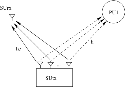
With reference to Fig. 1, we consider a point-to-point SU MISO communication system, where the SU has $N$ transmit antennas and a single receive antenna. The signal model of the SU can be represented as $y={\mbox{\boldmath$h$}}_{s}^{H}{\mbox{\boldmath$x$}}+n$, where $y$ and $x$ are the received and transmitted signals respectively, ${\mbox{\boldmath$h$}}_{s}$ denotes the $N\times 1$ channel response from the SU-Tx to the SU-Rx, and $n$ is independent and identically distributed (i.i.d.) Gaussian noise with zero mean and unit variance¹¹ 1 Since the SU receiver cannot differentiate the interference from the PU from the background noise, the term $n$ can be viewed as the summation of the interference and the noise. The variance of $n$ does not influence the algorithms discussed later. Moreover, the variance of $n$ can be measured at the SU receiver [13]. . Suppose that the PU has one receive antenna. The channel response from the SU-Tx to the PU is denoted by an $N\times 1$ vector $h$. Further, assume that the SU-Tx has perfect CSI for its own link, i.e., ${\mbox{\boldmath$h$}}_{s}$ is perfectly known at the SU-Tx. However, due to the loose cooperation between the SU and the PU, only partial CSI about $h$ is assumed to be available at the SU-Tx. We assume that ${\mbox{\boldmath$h$}}_{0}$ and $R$ are the mean and covariance of $h$, respectively²² 2 Due to the cognitive property, we assume that the SU can obtain the pilot signal from the PU, and thus can detect the channel information from the PU to the SU. Moreover, since the SU shares the same spectrum with the PU, based on the channel from the PU to the SU, the statistics of the channel from the SU to the PU can be obtained [15]. Therefore, we can assume that ${\mbox{\boldmath$h$}}_{0}$ and $R$ are known to the SU.. In previous work [10, 16, 15, 17], partial CSI has been considered in two extreme cases in a non-CR setting. One is the mean feedback case, ${\mbox{\boldmath$R$}}=\sigma^{2}{\mbox{\boldmath$I$}}$, where $\sigma^{2}$ can be viewed as the variance of the estimation error; and the other is the covariance feedback case, where ${\mbox{\boldmath$h$}}_{0}$ is a zero vector. In this paper, we study the case where the SU-Tx knows both the mean and covariance of $h$ in a CR setting.

The objective of this paper is to determine the optimal transmit signal covariance matrix such that the information rate of the SU link is maximized while the QoS of the PU is guaranteed under a robust design scenario, i.e., the instantaneous interference power for the PU should remain below a given threshold for all the $h$ in the uncertain region. Mathematically, the problem is formulated as follows:

where $S$ is the transmit signal covariance matrix, $\bar{P}$ is the transmit power budget, $P_{{t}}$ is the interference threshold of the PU, and $\epsilon$ is a positive constant. The parameter $\epsilon$ characterizes the uncertainty of $h$ at the SU. According to the definition of the uncertainty in [18], $\mathbf{P1}$ belongs to a type of ellipsoid uncertainty problem, i.e., the uncertain parameter $h$ is confined in a range of an ellipsoid $\mathcal{H}$, where $\mathcal{H}:\{{\mbox{\boldmath$h$}}|({\mbox{\boldmath$h$}}-{\mbox{\boldmath$h$}}_{0})^{H}{\mbox{\boldmath$R$}}^{-1}({\mbox{\boldmath$h$}}-{\mbox{\boldmath$h$}}_{0})\leq\epsilon\}$. Thus, the optimal solution of problem $\mathbf{P1}$ can guarantee the interference power constraint of the PU for all the ${\mbox{\boldmath$h$}}\in\mathcal{H}$, and thus the robustness of $\mathbf{P1}$ is in the worst case sense [19], i.e., in the worst case channel realization, the interference constraint should also be satisfied. If the primary transmission does not exist, then the interference constraint is excluded, and thus the problem reduces to a trivial beamforming problem. Hence, we only focus on the case where the both PU and SU transmission exist.

Since problem $\mathbf{P1}$ has a finite number of decision variable $S$, and is subjected to an infinite number of constraints with respect to the compact set $\mathcal{H}$, problem $\mathbf{P1}$ is an SIP problem [20]. One obvious approach for an SIP problem is to transform it into a finite constraint problem. However, there is no universal algorithm to determine the equivalent finite constraints such that the transformed problem has the same solution as the original SIP problem. In the following section, we first study several important properties of problem $\mathbf{P1}$, which would be used to transform the SIP problem into its equivalent finite constraint counterpart.

The maximization problem $\mathbf{P1}$ is a convex optimization problem, and thus has a unique optimal solution. The following lemma presents a key property of the optimal solution of problem $\mathbf{P1}$ (see Appendix A for the proof).

According to Lemma 1, a necessary and sufficient condition for the optimal solution of problem $\mathbf{P1}$ is presented as follows (refer to Appendix B for the proof).

In the following lemma (see Appendix C for the proof), the optimal beamforming vector ${\mbox{\boldmath$v$}}_{\text{opt}}$ is shown to lie in a two-dimensional (2-D) space spanned by ${\mbox{\boldmath$h$}}_{0}$ and the projection of ${\mbox{\boldmath$h$}}_{s}$ into the null space of ${\mbox{\boldmath$h$}}_{0}$. Define $\hat{{\mbox{\boldmath$h$}}}={\mbox{\boldmath$h$}}_{0}/\|{\mbox{\boldmath$h$}}_{0}\|$ and $\hat{{\mbox{\boldmath$h$}}}_{\perp}={\mbox{\boldmath$h$}}_{\perp}/\|{\mbox{\boldmath$h$}}_{\perp}\|$, where ${\mbox{\boldmath$h$}}_{\perp}={\mbox{\boldmath$h$}}_{s}-(\hat{{\mbox{\boldmath$h$}}}^{H}{\mbox{\boldmath$h$}}_{s})\hat{{\mbox{\boldmath$h$}}}$. Hence, we have ${\mbox{\boldmath$h$}}_{s}=a_{h_{s}}\hat{{\mbox{\boldmath$h$}}}+b_{h_{s}}\hat{{\mbox{\boldmath$h$}}}_{\perp}$ with $a_{h_{s}},b_{h_{s}}\in\mathbb{R}$.

In this section, we solve problem $\mathbf{P1}$ via a standard interior point algorithm [19, 21, 22]. We first transform the SIP problem into a finite constraint problem, and further transform it into a standard SOCP form, which can be solved by using a standard software package such as SeDuMi [23]. One key observation is that if $\max_{{\mbox{\small\boldmath$h$}}\in\mathcal{H}(\epsilon)}~{\mbox{\boldmath$h$}}^{H}{\mbox{\boldmath$S$}}{\mbox{\boldmath$h$}}\leq P_{{t}}$, i.e., the worst case interference constraint of $\mathbf{P1}$ is satisfied, then the interference constraint of $\mathbf{P1}$ holds. Combining this observation with Lemma 1, problem $\mathbf{P1}$ can be transformed as:

where $\mathcal{H}(\epsilon):=\{{\mbox{\boldmath$h$}}|{\mbox{\boldmath$h$}}={\mbox{\boldmath$h$}}_{0}+{\mbox{\boldmath$h$}}_{1}\}$. It is clear that maximizing $\log(1+p{\mbox{\boldmath$h$}}_{s}^{H}{\mbox{\boldmath$v$}}{\mbox{\boldmath$v$}}^{H}{\mbox{\boldmath$h$}}_{s})$ is equivalent to maximizing $|\sqrt{p}{\mbox{\boldmath$h$}}_{s}^{H}{\mbox{\boldmath$v$}}|$. By defining ${\mbox{\boldmath$w$}}=\sqrt{p}{\mbox{\boldmath$v$}}$, the objective function can be rewritten as $|{\mbox{\boldmath$h$}}_{s}^{H}{\mbox{\boldmath$w$}}|$. Similarly, the interference power can be expressed as $|{\mbox{\boldmath$h$}}^{H}{\mbox{\boldmath$w$}}|^{2}$. Thus, problem $\mathbf{P2}$ can be further transformed to

According to the definition of $\mathcal{H}(\epsilon)$, we can rewrite the worst-case constraint in (5) as

where $\mathcal{H}_{1}(\epsilon):=\{{\mbox{\boldmath$h$}}_{1}|{\mbox{\boldmath$h$}}_{1}^{H}{\mbox{\boldmath$R$}}^{-1}{\mbox{\boldmath$h$}}_{1}\leq\epsilon\}$. By applying the triangle inequality and the fact that $\sqrt{\epsilon}\|{\mbox{\boldmath$Q$}}{\mbox{\boldmath$w$}}\|=\max|{\mbox{\boldmath$h$}}_{1}^{H}{\mbox{\boldmath$w$}}|$ for ${\mbox{\boldmath$h$}}_{1}\in\mathcal{H}_{1}(\epsilon)$ (refer to Appendix D for details), the interference power can be transformed as follows:

where ${\mbox{\boldmath$Q$}}=\mathbf{\Delta}^{-1/2}{\mbox{\boldmath$U$}}$ with $\mathbf{\Delta}$ and $U$ being obtained by the eigenvalue decomposition of ${\mbox{\boldmath$R$}}^{-1}$ as ${\mbox{\boldmath$R$}}^{-1}={\mbox{\boldmath$U$}}^{H}\mathbf{\Delta}{\mbox{\boldmath$U$}}$. Moreover, since the arbitrary phase rotation of $w$ does not change the value of the objective function or the constraints, according to Remark 1 and Lemma 3, we can assume that $w$, ${\mbox{\boldmath$h$}}_{s}$, and ${\mbox{\boldmath$h$}}_{0}$ have the same phase, i.e.,

Hence, the interference constraint can be transformed into two second order cone inequalities as follows

By combining (5), (9), with (8), problem $\mathbf{P1}$ is transformed into the standard SOCP problem as follows

Since the parameters ${\mbox{\boldmath$h$}}_{s}$ and ${\mbox{\boldmath$h$}}_{0}$, and the variable $w$ in (10) have complex values, we first convert them to its corresponding real-valued form in order to simplify the solution. Define $\tilde{{\mbox{\boldmath$w$}}}:=[\text{Re}\{{\mbox{\boldmath$w$}}\}^{T},\text{Im}\{{\mbox{\boldmath$w$}}\}^{T}]^{T}$, $\tilde{{\mbox{\boldmath$h$}}}_{0}:=[\text{Re}\{{\mbox{\boldmath$h$}}_{0}\}^{T},\text{Im}\{{\mbox{\boldmath$h$}}_{0}\}^{T}]^{T}$, $\tilde{{\mbox{\boldmath$h$}}}_{s}:=[\text{Re}\{{\mbox{\boldmath$h$}}_{s}\}^{T},\text{Im}\{{\mbox{\boldmath$h$}}_{s}\}^{T}]^{T}$, $\check{{\mbox{\boldmath$h$}}}_{0}:=[\text{Im}\{{\mbox{\boldmath$h$}}_{0}\}^{T},-\text{Re}\{{\mbox{\boldmath$h$}}_{0}\}^{T}]^{T}$, and $\tilde{{\mbox{\boldmath$Q$}}}:=\left[\begin{array}[]{ccc}\text{Re}\{{\mbox{\boldmath$Q$}}\}~-&\text{Im}\{{\mbox{\boldmath$Q$}}\}\\ \text{Im}\{{\mbox{\boldmath$Q$}}\}&\text{Re}\{{\mbox{\boldmath$Q$}}\}\\ \end{array}\right].$

We then can rewrite the standard SOCP problem (10) as

Problem (11) can be solved by a standard interior point program SeDuMi [23], which has a polynomial complexity. In the next section, we develop an analytical algorithm to solve problem $\mathbf{P1}$, which reduces the complexity of the interior point based algorithm substantially.

In this section, we present a geometric approach to problem $\mathbf{P1}$. We begin by studying a special case, the mean feedback case, i.e., ${\mbox{\boldmath$R$}}=\sigma^{2}{\mbox{\boldmath$I$}}$. Due to its special geometric structure, the mean feedback case problem can be solved via a closed-form algorithm. We next show that problem $\mathbf{P1}$ can be transformed into an optimization problem similar to the mean feedback case. Based on the closed-form solution derived for the mean feedback case, the analytical solution to problem $\mathbf{P1}$ with a general form of a covariance matrix $R$ is presented in Subsection V-B.

Computer simulations are provided in this section to evaluate the performance of the proposed algorithms. In the simulations, it is assumed that the entries of the channel vectors ${\mbox{\boldmath$h$}}_{s}$ and ${\mbox{\boldmath$h$}}_{0}$ are modeled as independent circularly symmetric complex Gaussian random variables with zero mean and unit variance. Moreover, we denote by $l_{1}$ the distance between the SU-Tx and the SU-Rx, and by $l_{2}$ the distance between the SU-Tx and the PU. It is assumed that the same path loss model is used to describe the transmissions from the SU-Tx to the SU-Rx and to the PU, and the path loss exponent is chosen to be $4$. The noise power is chosen to be $1$, and the transmit power and interference power are defined in dB relative to the noise power. For all cases, we choose $P_{{t}}=0$ dB.

In this paper, the robust cognitive beamforming design problem has been investigated, for the SU MISO communication system in which only partial CSI of the link from the SU-Tx to the PU is available at the SU-Tx. The problem can be formulated as an SIP optimization problem. Two approaches have been proposed to obtain the optimal solution of the problem; one approach is based on a standard interior point algorithm, while the other approach solves the problem analytically. Simulation examples have been used to present a comparison of the two approaches as well as to study the effectiveness and activeness of imposed constraints.

This work initiates research in robust design of cognitive radios. We are currently extending these methods to the more general case with multiple receive antennas and multiple PUs. Other interesting extensions include more practical scenarios, such as the case in which the SU channel information is also partially known at the SU-Tx.

References

• [1] Federal Communications Commission, “Facilitating opportunities for flexible, efficient, and reliable spectrum use employing cognitive radio technologies, notice of proposed rule making and order, fcc 03-322,” Dec. 2003.
• [2] J. Mitola and G. Q. Maguire, “Cognitive radios: Making software radios more personal,” IEEE Personal Communications, vol. 6, no. 4, pp. 13–18, Aug. 1999.
• [3] S. Haykin, “Cognitive radio: Brain-empowered wireless communications,” IEEE J. Select. Areas Commun., vol. 23, no. 2, pp. 201–202, Feb. 2005.
• [4] Z. Quan, S. Cui, and A. Sayed, “Optimal linear cooperation for spectrum sensing in cognitive radio networks,” IEEE J. Select. Topics in Signal Processing, vol. 2, no. 1, pp. 28–40, Feb. 2008.
• [5] F. Wang, M. Krunz, and S. Cui, “Price-based spectrum management in cognitive radio networks,” IEEE J. Select. Topics in Signal Processing, vol. 2, no. 1, pp. 74–87, Feb. 2008.
• [6] M. Gastpar, “On capacity under receive and spatial spectrum-sharing constraints,” IEEE Trans. Inform. Theory, vol. 53, no. 2, pp. 471–487, Feb. 2007.
• [7] A. Ghasemi and E. S. Sousa, “Fundamental limits of spectrum-sharing in fading environments,” IEEE Trans. Wireless Commun., vol. 6, no. 2, pp. 649–658, Feb. 2007.
• [8] Y.-C. Liang, Y. Zeng, E. Peh, and A. Hoang, “Sensing-throughput tradeoff for cognitive radio networks,” IEEE Trans. Wireless Commun., vol. 7, no. 4, pp. 1326–1337, Apr. 2008.
• [9] S. Zhou and G. B. Giannakis, “Optimal transmitter eigen-beamforming and space-time block coding based on channel mean feedback,” IEEE Trans. Signal Processing, vol. 50, no. 10, pp. 2599–2613, Oct. 2002.
• [10] E. Visotsky and U. Madhow, “Space-time transmit precoding with imperfect feedback,” IEEE Trans. Inform. Theory, vol. 47, no. 6, pp. 2632–2639, Sept. 2001.
• [11] S. A. Jafar and A. J. Goldsmith, “Transmitter optimization and optimality of beamforming for multiple antenna systems with imperfect feedback,” IEEE Trans. Wireless Commun., vol. 3, no. 4, pp. 1165–1175, July 2004.
• [12] K. K. Mukkavilli, A. Sabharwal, E. Erkip, and B. Aazhang, “On beamforming with finite rate feedback in multiple antenna systems,” IEEE Trans. Inform. Theory, vol. 49, no. 10, pp. 2562–2579, Oct. 2003.
• [13] L. Zhang, Y.-C. Liang, and Y. Xin, “Joint beamforming and power allocation for multiple access channels in cognitive radio networks,” IEEE J. Select. Areas Commun., vol. 26, no. 1, pp. 38–51, Jan. 2008.
• [14] R. Zhang and Y.-C. Liang, “Exploiting multi-antennas for opportunistic spectrum sharing in cognitive radio networks,” IEEE J. Select. Topics in Signal Processing, vol. 2, no. 1, pp. 88–102, Feb. 2008.
• [15] Y.-C. Liang and F. P. S. Chin, “Downlink channel covariance matrix (DCCM) estimation and its applications in wireless DS-CDMA systems,” IEEE J. Select. Areas Commun., vol. 19, no. 2, pp. 222–232, Feb. 2001.
• [16] S. Srinivasa and S. A. Jafar, “The optimality of transmit beamforming: a unified view,” IEEE Trans. Inform. Theory, vol. 53, no. 4, pp. 1558–1564, Apr. 2007.
• [17] E. Jorswieck and H. Boche, “Optimal transmission with imperfect channel state information at the transmit antenna array,” Wireless Pers. Commun., vol. 27, no. 1, pp. 33–56, Jan. 2003.
• [18] A. Ben-Tal and A. Nemirovski, “Selected topics in robust convex optimization,” Mathematical Programming, vol. 1, no. 1, pp. 125–158, 2007.
• [19] S. Boyd and L. Vandenberghe, Convex Optimization. Cambridge, UK: Cambridge University Press, 2004.
• [20] R. Reemtsen and J.-J. Ruckmann, Semi-Infinite Programming. Boston: Kluwer Academic Publishers, 1998.
• [21] S. Vorobyov, A. Gershman, and Z.-Q. Luo, “Robust adaptive beamforming using worst-case performance optimization: A solution to the signal mismatch problem,” IEEE Trans. Signal Processing, vol. 51, no. 2, pp. 313–323, Feb. 2003.
• [22] Z.-Q. Luo and W. Yu, “An introduction to convex optimization for communications and signal processing,” IEEE J. Select. Areas Commun., vol. 24, no. 8, pp. 1426–1438, Aug. 2006.
• [23] J. F. Sturm, “Using sedumi 1.02, a MATLAB toolbox for optimization over symmetric cones,” Optim. Meth. Softw., vol. 11, pp. 625–653, 1999.
TABLE I: The algorithm for SP2.
Algorithm 1
1. Compute βopt\beta_{\text{opt}} through (25),
2. Compute poptp_{\text{opt}} according to (21),
3. Compute 𝒗opt{\mbox{\boldmath$v$}}_{\text{opt}} according to (26),
4. 𝑺opt=popt​𝒗opt​𝒗optH{\mbox{\boldmath$S$}}_{\text{opt}}=p_{\text{opt}}{\mbox{\boldmath$v$}}_{\text{opt}}{\mbox{\boldmath$v$}}_{\text{opt}}^{H}.
TABLE II: The algorithm for problem 𝐏𝟑\mathbf{P3} in the case where two constraints are satisfied simultaneously.
Algorithm 2
1. Compute βopt\beta_{\text{opt}} through (30),
2. Based on (26), compute 𝒗opt{\mbox{\boldmath$v$}}_{\text{opt}},
3. 𝑺opt=P¯​𝒗opt​𝒗optH{\mbox{\boldmath$S$}}_{\text{opt}}=\bar{P}{\mbox{\boldmath$v$}}_{\text{opt}}{\mbox{\boldmath$v$}}_{\text{opt}}^{H}.
TABLE III: The complete algorithm for problem 𝐏𝟑\mathbf{P3}.
Algorithm 3
1. Compute the optimal solution 𝑺1=P¯​𝒉s​𝒉sH/‖𝒉s‖2{\mbox{\boldmath$S$}}_{1}=\bar{P}{\mbox{\boldmath$h$}}_{s}{\mbox{\boldmath$h$}}_{s}^{H}/\|{\mbox{\boldmath$h$}}_{s}\|^{2} for 𝐒𝐏𝟏\mathbf{SP1},
2. Compute the optimal solution 𝑺2{\mbox{\boldmath$S$}}_{2} for 𝐒𝐏𝟐\mathbf{SP2} via Algorithm 1,
3. If 𝑺1{\mbox{\boldmath$S$}}_{1} satisfies the interference constraint, then 𝑺1{\mbox{\boldmath$S$}}_{1} is the optimal solution,
4. Elsif 𝑺2{\mbox{\boldmath$S$}}_{2} satisfies the transmit power constraint, then 𝑺2{\mbox{\boldmath$S$}}_{2} is the optimal solution,
5. Otherwise compute the optimal solution via Algorithm 2.
TABLE IV: The algorithm for problem 𝐏𝟒\mathbf{P4} in the case where two constraints are satisfied simultaneously.
Algorithm 4
1. Compute β¯\bar{\beta} via (41), and compute 𝒗¯\bar{{\mbox{\boldmath$v$}}} via (37),
2. Based on the relationship between 𝒗¯\bar{{\mbox{\boldmath$v$}}} and 𝒗v, compute 𝒗opt{\mbox{\boldmath$v$}}_{\text{opt}},
TABLE V: The complete algorithm for problem 𝐏𝟏\mathbf{P1}.
Algorithm 5
1. Compute the optimal solution 𝑺3=P¯​𝒉s​𝒉sH/‖𝒉s‖2{\mbox{\boldmath$S$}}_{3}=\bar{P}{\mbox{\boldmath$h$}}_{s}{\mbox{\boldmath$h$}}_{s}^{H}/\|{\mbox{\boldmath$h$}}_{s}\|^{2} for 𝐒𝐏𝟑\mathbf{SP3},
2. Compute the optimal solution 𝑺4{\mbox{\boldmath$S$}}_{4} for 𝐒𝐏𝟒\mathbf{SP4} via Algorithm 4,
3. If 𝑺3{\mbox{\boldmath$S$}}_{3} satisfies the interference constraint, then 𝑺3{\mbox{\boldmath$S$}}_{3} is the optimal solution,
4. Elsif 𝑺4{\mbox{\boldmath$S$}}_{4} satisfies the transmit power constraint, then 𝑺4{\mbox{\boldmath$S$}}_{4} is the optimal solution,
5. Otherwise compute the optimal solution through Algorithm 4.
Refer to caption
Fig. 1: The system model for the MISO SU network coexisting with one PU.
Fig. 2: The geometric explanation of Lemma 3. The ellipse is the projection of 𝒉:={(𝒉−𝒉0)H𝑹−1(𝒉−𝒉0)=ϵ}{\mbox{\boldmath$h$}}:=\{({\mbox{\boldmath$h$}}-{\mbox{\boldmath$h$}}_{0})^{H}{\mbox{\boldmath$R$}}^{-1}({\mbox{\boldmath$h$}}-{\mbox{\boldmath$h$}}_{0})=\epsilon\} on the plane spanned by 𝒉^\hat{{\mbox{\boldmath$h$}}} and 𝒉^⟂\hat{{\mbox{\boldmath$h$}}}_{\perp}.
Fig. 3: The geometric explanation of problem 𝐏𝟑\mathbf{P3}. The circle is the projection of 𝒉:={∥𝒉−𝒉0∥2=0}{\mbox{\boldmath$h$}}:=\{\|{\mbox{\boldmath$h$}}-{\mbox{\boldmath$h$}}_{0}\|^{2}=0\} on the plane spanned by 𝒉^\hat{{\mbox{\boldmath$h$}}} and 𝒉^⟂\hat{{\mbox{\boldmath$h$}}}_{\perp}.
Fig. 4: Comparison of the results obtained by the SOCP algorithm and Algorithm 3.
Fig. 5: Comparison of the results obtained by the SOCP algorithm and Algorithm 5.
Fig. 6: Effect of l2/l1l_{2}/l_{1} on the achievable rate of the CR network (ϵ=1\epsilon=1, N=3N=3).
Fig. 7: Comparison of the rate under different constraints of problem 𝐏𝟏\mathbf{P1}. (i) the maximal rate subject to interference constraint and transmit power constraint simultaneously; (ii) the maximal rate subject to a single transmit power constraint; (iii) the maximal rate subject to a single interference constraint.