Performance of LDPC Codes Under
Faulty Iterative Decoding

Lav R. Varshney ^†^†thanks: Manuscript prepared May 2008; revised April 2009, May 2010. This work was supported in part by a National Science Foundation Graduate Research Fellowship and was performed in part when the author was with l’École Polytechnique Fédérale de Lausanne. The material in this paper was presented in part at the Information Theory Workshop, Lake Tahoe, CA, September 2007.^†^†thanks: L.˜R.˜Varshney is with the Department of Electrical Engineering and Computer Science, the Laboratory for Information and Decision Systems, and the Research Laboratory of Electronics, Massachusetts Institute of Technology, Cambridge, MA, 02139 USA (e-mail: lrv@mit.edu).

Abstract

Departing from traditional communication theory where decoding algorithms are assumed to perform without error, a system where noise perturbs both computational devices and communication channels is considered here. This paper studies limits in processing noisy signals with noisy circuits by investigating the effect of noise on standard iterative decoders for low-density parity-check codes. Concentration of decoding performance around its average is shown to hold when noise is introduced into message-passing and local computation. Density evolution equations for simple faulty iterative decoders are derived. In one model, computing nonlinear estimation thresholds shows that performance degrades smoothly as decoder noise increases, but arbitrarily small probability of error is not achievable. Probability of error may be driven to zero in another system model; the decoding threshold again decreases smoothly with decoder noise. As an application of the methods developed, an achievability result for reliable memory systems constructed from unreliable components is provided.

Index Terms:

Low-density parity-check codes, communication system fault tolerance, density evolution, decoding, memories

I Introduction

The basic goal in channel coding is to design encoder-decoder pairs that allow reliable communication over noisy channels at information rates close to capacity [1]. The primary obstacle in the quest for practical capacity-achieving codes has been decoding complexity [2, 3, 4]. Low-density parity-check (LDPC) codes have, however, emerged as a class of codes that have performance at or near the Shannon limit [5, 6] and yet are sufficiently structured as to have decoders with circuit implementations [7, 8, 9].

In addition to decoder complexity, decoder reliability may also limit practical channel coding.¹¹ 1 One may also consider the effect of encoder complexity [10], however encoder noise need not be explicitly considered, since it may be incorporated into channel noise, using the noise combining argument suggested by Fig. 3. In Shannon’s schematic diagram of a general communication system [1, Fig. 1] and in the traditional information and communication theories that have developed within the confines of that diagram, noise is localized in the communication channel. The decoder is assumed to operate without error. Given the possibility of unreliable computation on faulty hardware, there is value in studying error-prone decoding. In fact Hamming’s original development of parity-check codes was motivated by applications in computing rather than in communication [11].

The goal of this paper is to investigate limits of communication systems with noisy decoders and has dual motivations. The first is the eminently practical motivation of determining how well error control codes work when decoders are faulty. The second is the deeper motivation of determining fundamental limits for processing unreliable signals with unreliable computational devices, illustrated schematically in Fig. 1. The motivations are intertwined. As noted by Pierce, “The down-to-earth problem of making a computer work, in fact, becomes tangled with this difficult philosophical problem: ‘What is possible and what is impossible when unreliable circuits are used to process unreliable information?’” [12].

Refer to caption — Fig. 1: Schematic diagram of an information system that processes unreliable signals with unreliable circuits.

A first step in understanding these issues is to analyze a particular class of codes and decoding techniques: iterative message-passing decoding algorithms for LDPC codes. When the code is represented as a factor graph, algorithm computations occur at nodes and algorithm communication is carried out over edges. Correspondence between the factor graph and the algorithm is not only a tool for exposition but also the way decoders are implemented [7, 8, 9]. In traditional performance analysis, the decoders are assumed to work without error. In this paper, there will be transient local computation and message-passing errors, whether the decoder is analog or digital.

When the decoder itself is noisy, one might believe that achieving arbitrarily small probability of error (Shannon reliability) is not possible, but this is indeed possible for certain sets of noisy channels and noisy decoders. This is shown by example. For other sets of noisy channels and noisy decoders, Shannon reliability is not achievable, but error probability tending to extremely small values is achievable. Small probability of error, $\eta$ , is often satisfactory in practice, and so $\eta$ -reliable performance is also investigated. Decoding thresholds at $\eta$ -reliability decrease smoothly with increasing decoder noise. Communication systems may display graceful degradation with respect to noise levels in the decoder.

The remainder of the paper is organized as follows. Section II reviews motivations and related work. Section III formalizes notation and Section IV gives concentration results that allow the density evolution method of analysis, generalizing results in [13]. A noisy version of the Gallager A decoder for processing the output of a binary symmetric channel is analyzed in Section V, where it is shown that Shannon reliability is unattainable. In Section VI, a noisy decoder for AWGN channels is analyzed. For this model, the probability of error may be driven to zero and the decoding threshold degrades smoothly as a function of decoder noise. As an application of the results of Section V, Section VII precisely characterizes the information storage capacity of a memory built from unreliable components. Section VIII provides some conclusions.

II Background

II-A Practical Motivations

Although always present [11, 14], recent technological trends in digital circuit design bring practical motivations to the fore [15, 16, 17]. The 2008 update of the International Technology Roadmap for Semiconductors (ITRS)²² 2 The overall objective of the ITRS is to present the consensus of the semiconductor industry on the best current estimate of research and development needs for the next fifteen years. points out that for complementary metal-oxide-silicon (CMOS) technology, increasing power densities, decreasing supply voltages, and decreasing sizes have increased sensitivity to cosmic radiation, electromagnetic interference, and thermal fluctuations. The ITRS further says that an ongoing shift in the manufacturing paradigm will dramatically reduce costs but will lead to more transient failures of signals, logic values, devices, and interconnects. Device technologies beyond CMOS, such as single-electron tunnelling technology [18], carbon-based nanoelectronics [19], and chemically assembled electronic nanocomputers [20], are also projected to enter production, but they all display erratic, random device behavior [21, 22].

Analog computations are always subject to noise [23, 24]. Similar issues arise when performing real-valued computations on digital computers since quantization, whether fixed-point or floating-point, is often well-modeled as bounded, additive stochastic noise [25].

II-B Coding and Computing

Information and communication theory have provided limits for processing unreliable signals with reliable circuits [1, 26, 13], whereas fault-tolerant computing theory has provided limits for processing reliable signals (inputs) with unreliable circuits [27, 28, 12, 29, 30, 31]. This work brings the two together.

A brief overview of terms and concepts from fault-tolerant computing, based on [32, 33], is now provided. A fault is a physical defect, imperfection, or flaw that occurs within some hardware or software component. An error is the informational manifestation of a fault. A permanent fault exists indefinitely until corrective action is taken, whereas a transient fault appears and disappears in a short period of time. Noisy circuits in which the interconnection pattern of components are trees are called formulas [34, 35].

In an error model, the effects of faults are given directly in the informational universe. For example, the basic von Neumann model of noisy circuits [27] models transient faults in logic gates and wires as message and node computation noise that is both spatially and temporally independent; this has more recently also been called the Hegde-Shanbhag model [36], after [37]. This error model is used here. Error models of permanent faults [38, 39] or of miswired circuit interconnection [28, 40] have been considered elsewhere. Such permanent errors in decoding circuits may be interpreted as either changing the factor graph used for decoding or as introducing new potentials into the factor graph; the code used by the encoder and the code used by the decoder are different.

There are several design philosophies to combat faults. Fault avoidance seeks to make physical components more reliable. Fault masking seeks to prevent faults from introducing errors. Fault tolerance is the ability of a system to continue performing its function in the presence of faults. This paper is primarily concerned with fault tolerance, but Section VII considers fault masking.

II-C Related Work

Empirical characterizations of message-passing decoders have demonstrated that probability of error performance does not change much when messages are quantized at high resolution [26]. Even algorithms that are coarsely quantized versions of optimal belief propagation show little degradation in performance [41, 13, 42, 43, 44, 45, 46]. It should be emphasized, however, that fault-free, quantized decoders differ significantly from decoders that make random errors.³³ 3 Randomized algorithms [47] and stochastic computation [48] (used for decoding in [49]) make use of randomness to increase functionality, but the randomness is deployed in a controlled manner. The difference is similar to that between control systems with finite-capacity noiseless channels and control systems with noisy channels of equal capacity [50]. Seemingly the only previous work on message-passing algorithms with random errors is [51], which deals with problems in distributed inference.⁴⁴ 4 If the graphical model of the code and the graph of noisy communication links in a distributed system coincide, then the distributed inference problem and the message-passing decoding problem can be made to coincide.

The information theoretic problem of mismatch capacity [52] and its analog for iterative decoding [53] deal with scenarios where an incorrect decoding metric is used. This may arise, e.g., due to incorrect estimation of the channel noise power. For message-passing decoding algorithms, mismatch leads to incorrect parameters for local computations. These are permanent faults rather than the kind of transient faults considered in this paper.

Noisy LDPC decoders were previously analyzed in the context of designing reliable memories from unreliable components [54, 55] (revisited in Section VII), using Gallager’s original methods [26]. Several LPDC code analysis tools have since been developed, including simulation [56], expander graph arguments [57, 58], EXIT charts [59, 60], and density evolution [61, 13, 62]. This work generalizes asymptotic characterizations developed by Richardson and Urbanke for noiseless decoders [13], showing that density evolution is applicable to faulty decoders. Expander graph arguments have also been extended to the case of noisy decoding in a paper [63] that appeared concurrently with the first presentation of this work [64]. Note that previous works have not even considered the possibility that Shannon reliability is achievable with noisy decoding.

III Codes, Decoders, and Performance

This section establishes the basic notation of LDPC channel codes and message-passing decoders for communication systems depicted in Fig. 1. It primarily follows established notation in the field [13, 65], and will therefore be brief. Many of the notational conventions are depicted schematically in Fig. 2 using a factor graph-based decoder implementation.

Consider the standard ensemble of $({d_{\tt{v}}},{d_{\tt{c}}})$ -regular LDPC codes of length $n$ , $\mathcal{C}^{n}({d_{\tt{v}}},{d_{\tt{c}}})$ , defined by a uniform measure on the set of labeled bipartite factor graphs with variable node degree ${d_{\tt{v}}}$ and check node degree ${d_{\tt{c}}}$ .⁵⁵ 5 A factor graph determines an “ordered code,” but the opposite is not true [66]. Moreover, since codes are unordered objects, several “ordered codes” are in fact the same code. There are $n$ variable nodes corresponding to the codeword letters and $n{d_{\tt{v}}}/{d_{\tt{c}}}$ check nodes corresponding to the parity check constraints. The design rate of the code is $1-{d_{\tt{v}}}/{d_{\tt{c}}}$ , though the actual rate might be higher since not all checks may be independent; the true rate converges to the design rate for large $n$ [65, Lemma 3.22]. One may also consider irregular codes, $\mathcal{C}^{n}(\lambda,\rho)$ characterized by the degree distribution pair $(\lambda,\rho)$ . Generating functions of the variable node and check node degree distributions, $\lambda(\zeta)$ and $\rho(\zeta)$ , are functions of the form $\lambda(\zeta)=\sum_{i=2}^{\infty}\lambda_{i}\zeta^{i-1}$ and $\rho(\zeta)=\sum_{i=2}^{\infty}\rho_{i}\zeta^{i-1}$ , where $\lambda_{i}$ and $\rho_{i}$ specify the fraction of edges that connect to nodes with degree $i$ . The design rate is $1-\int_{0}^{1}\rho(\zeta)d\zeta/\int_{0}^{1}\lambda(\zeta)d\zeta$ .

In the communication system of Fig. 1, a codeword is selected by the transmitter and is sent through the noisy channel. Channel input and output letters are denoted $X\in\mathcal{X}$ and $Y\in\mathcal{Y}$ . Since binary linear codes are used, $\mathcal{X}$ can be taken as $\{\pm 1\}$ . The receiver contains a noisy message-passing decoder, which is used to process the channel output codeword to produce an estimate of $X$ that is denoted $\hat{X}$ . The goal of the receiver is to recover the channel input codeword with low probability of error. Throughout this work, probability of bit error $P_{e}$ is used as the performance criterion;⁶⁶ 6 An alternative would be to consider block error probability, however an exact evaluation of this quantity is difficult due to the dependence between different symbols of a codeword, even if the bit error probability is the same for all symbols in the codeword [67].

P_{e}=\Pr[X\neq\hat{X}]\mbox{.}

The message-passing decoder works in iterative stages and the iteration time is indexed by $\ell=0,1,\ldots$ . Within the decoder, at time $\ell=0$ , each variable node has a realization of $Y$ , $y_{i}$ . A message-passing decoder exchanges messages between nodes along wires. First each variable node sends a message to a neighboring check node over a noisy messaging wire. Generically, sent messages are denoted as $\nu_{\tt{v}\to\tt{c}}$ , message wire noise realizations as $w_{\tt{v}\to\tt{c}}$ , and received messages as $\mu_{\tt{v}\to\tt{c}}$ : assume without loss of generality that $\nu_{\tt{v}\to\tt{c}}$ , $w_{\tt{v}\to\tt{c}}$ , and $\mu_{\tt{v}\to\tt{c}}$ are drawn from a common messaging alphabet $\mathcal{M}$ .

Each check node processes received messages and sends back a message to each neighboring variable node over a noisy message wire. The noisiness of the check node processing is generically denoted by an input random variable $U_{\tt{c}}\in\mathcal{U}$ . The check node computation is denoted $\Phi^{(\ell)}:\mathcal{M}^{{d_{\tt{c}}}-1}\times\mathcal{U}\mapsto\mathcal{M}$ . The notations $\nu_{\tt{c}\to\tt{v}}$ , $\mu_{\tt{c}\to\tt{v}}$ , and $w_{\tt{c}\to\tt{v}}$ are used for signaling from check node to variable node; again without loss of generality assume that $\nu_{\tt{c}\to\tt{v}},w_{\tt{c}\to\tt{v}},\mu_{\tt{c}\to\tt{v}}\in\mathcal{M}$ .

Each variable node now processes its $y_{i}$ and the messages it receives to produce new messages. The new messages are produced through possibly noisy processing, where the noise input is generically denoted $U_{\tt{v}}\in\mathcal{U}$ . The variable node computation is denoted $\Psi^{(\ell)}:\mathcal{Y}\times\mathcal{M}^{{d_{\tt{v}}}-1}\times\mathcal{U}\mapsto\mathcal{M}$ . Local computations and message-passing continue iteratively.

Message passing induces decoding neighborhoods, which involve nodes/wires that have communicated with one another. For a given node $\dot{n}$ , its neighborhood of depth $d$ is the induced subgraph consisting of all nodes reached and edges traversed by paths of length at most $d$ starting from $\dot{n}$ (including $\dot{n}$ ) and is denoted $\mathcal{N}_{\dot{n}}^{d}$ . The directed neighborhood of depth $d$ of a wire $\tt{v}\to\tt{c}$ , denoted by $\mathcal{N}_{\tt{v}\to\tt{c}}^{d}$ , is defined as the induced subgraph containing all wires and nodes on paths starting from the same place as $\tt{v}\to\tt{c}$ but different from $\tt{v}\to\tt{c}$ . Equivalently for a wire $\tt{c}\to\tt{v}$ , $\mathcal{N}_{\tt{c}\to\tt{v}}^{d}$ is the induced subgraph containing all wires and nodes on paths starting from the same place as $\tt{c}\to\tt{v}$ but different from $\tt{c}\to\tt{v}$ . If the induced subgraph (corresponding to a neighborhood) is a tree then the neighborhood is tree-like, otherwise it is not tree-like. The neighborhood is tree-like if and only if all involved nodes are distinct.

Note that only extrinsic information is used in node computations. Also note that in the sequel, all decoder noises ( $U_{\tt{c}}$ , $U_{\tt{v}}$ , $W_{\tt{v}\to\tt{c}}$ , and $W_{\tt{c}\to\tt{v}}$ ) will be assumed to be independent of each other, as in the von Neumann error model of faulty computing.

A communication system is judged by information rate, error probability, and blocklength. For fixed channels, information theory specifies the limits of these three parameters when optimizing over the unconstrained choice of codes and decoders; Shannon reliability is achievable for rates below capacity in the limit of increasing blocklength. When decoders are restricted to be noisy, tighter information theoretic limits are not known. Therefore comparing performance of systems with noisy decoders to systems using identical codes but noiseless decoders is more appropriate than comparing to Shannon limits.

Coding theory follows from information theory by restricting decoding complexity; analysis of noisy decoders follows from coding theory by restricting decoding reliability.

IV Density Evolution Concentration Results

Considering the great successes achieved by analyzing the noiseless decoder performance of ensembles of codes [61, 13, 65] rather than of particular codes [26], the same approach is pursued for noisy decoders. The first mathematical contribution of this work is to extend the method of analysis promulgated in [13] to the case of decoders with random noise.

Several facts that simplify performance analysis are proven. First, under certain symmetry conditions with wide applicability, the probability of error does not depend on which codeword is transmitted. Second, the individual performances of codes in an ensemble are, with high probability, the same as the average performance of the ensemble. Finally, this average behavior converges to the behavior of a code defined on a cycle-free graph. Performance analysis then reduces to determining average performance on an infinite tree: a noisy formula is analyzed in place of general noisy circuits.

For brevity, only regular LDPC codes are considered in this section, however the results can be generalized to irregular LDPC codes. In particular, replacing node degrees by maximum node degrees, the proofs stand mutatis mutandis. Similarly, only binary LDPC codes are considered; generalizations to non-binary alphabets also follow, as in [68].

IV-A Restriction to All-One Codeword

If certain symmetry conditions are satisfied by the system, then the probability of error is conditionally independent of the codeword that is transmitted. It is assumed throughout this section that messages in the decoder are in belief format.

Definition 1

A message in an iterative message-passing decoder for a binary code is said to be in belief format if the sign of the message indicates the bit estimate and the magnitude of the message is an increasing function of the confidence level. In particular, a positive-valued message indicates belief that a bit is $+1$ whereas a negative-valued message indicates belief that a bit is $-1$ . A message of magnitude $0$ indicates complete uncertainty whereas a message of infinite magnitude indicates complete confidence in a bit value.

Note, however, that it is not obvious that this is the best format for noisy message-passing [65, Appendix B.1]. The symmetry conditions can be restated for messages in other formats.

The several symmetry conditions are:

Definition 2 (Channel Symmetry)

A memoryless channel is binary-input output-symmetric if it satisfies

p(Y_{t}=y|X_{t}=1)=p(Y_{t}=-y|X_{t}=-1)

for all channel usage times $t=1,\ldots,n$ .

Definition 3 (Check Node Symmetry)

A check node message map is symmetric if it satisfies

\Phi^{(\ell)}(b_{1}\mu_{1},\ldots,b_{{d_{\tt{c}}}-1}\mu_{{d_{\tt{c}}}-1},b_{{d_{\tt{c}}}}u)=\Phi^{(\ell)}(\mu_{1},\ldots,\mu_{{d_{\tt{c}}}-1},u)\left(\prod\limits_{i=1}^{{d_{\tt{c}}}}b_{i}\right)

for any $\pm 1$ sequence $(b_{1},\ldots,b_{{d_{\tt{c}}}})$ . That is to say, the signs of the messages and the noise factor out of the map.

Definition 4 (Variable Node Symmetry)

A variable node message map is symmetric if it satisfies

\Psi^{(0)}(-\mu_{0},-u)=-\Psi^{(0)}(\mu_{0},u)

and

\Psi^{(\ell)}(-\mu_{0},-\mu_{1},\ldots,-\mu_{{d_{\tt{v}}}-1},-u)=-\Psi^{(\ell)}(\mu_{0},\mu_{1},\ldots,\mu_{{d_{\tt{v}}}-1},u)\mbox{,}

for $\ell\geq 1$ . That is to say, the initial message from the variable node only depends on the received value and internal noise and there is sign inversion invariance for all messages.

Definition 5 (Message Wire Symmetry)

Consider any message wire to be a mapping $\Xi:\mathcal{M}\times\mathcal{M}\to\mathcal{M}$ . Then a message wire is symmetric if

\mu=\Xi(\nu,w)=-\Xi(-\nu,-w)\mbox{,}

where $\mu$ is any message received at a node when the message sent from the opposite node is $\nu$ and $w$ is message wire noise with distribution symmetric about $0$ .

An example where the message wire symmetry condition holds is if the message wire noise $w$ is additive and symmetric about $0$ . Then $\mu=\nu+w=-(-\nu-w)$ and $w$ is symmetric about $0$ .

Theorem 1 (Conditional Independence of Error)

For a given binary linear code and a given noisy message-passing algorithm, let $P_{e}^{(\ell)}(\bf{x})$ denote the conditional probability of error after the $\ell$ th decoding iteration, assuming that codeword $\bf{x}$ was sent. If the channel and the decoder satisfy the symmetry conditions given in Definitions 2–5, then $P_{e}^{(\ell)}(\bf{x})$ does not depend on $\bf{x}$ .

Proof:

Modification of [13, Lemma 1] or [65, Lemma 4.92]. Appendix A gives details. ∎

Suppose a system meets these symmetry conditions. Since probability of error is independent of the transmitted codeword and since all LDPC codes have the all-one codeword in the codebook, one may assume without loss of generality that this codeword is sent. Doing so removes the randomness associated with transmitted codeword selection.

IV-B Concentration around Ensemble Average

The next simplification follows by seeing that the average performance of the ensemble of codes rather than the performance of a particular code may be studied, since all codes in the ensemble perform similarly. The performances of almost all LDPC codes closely match the average performance of the ensemble from which they are drawn. The average is over the instance of the code, the realization of the channel noise, and the realizations of the two forms of decoder noise. To simplify things, assume that the number of decoder iterations is fixed at some finite $\ell$ . Let $Z$ be the number of incorrect values held among all ${d_{\tt{v}}}n$ variable node-incident edges at the end of the $\ell$ th iteration (for a particular code, channel noise realization, and decoder noise realization) and let $E\left[{Z}\right]$ be the expected value of $Z$ . By constructing a martingale through sequentially revealing all of the random elements and then using the Hoeffding-Azuma inequality, it can be shown that:

Theorem 2 (Concentration Around Expected Value)

There exists a positive constant $\beta=\beta({d_{\tt{v}}},{d_{\tt{c}}},\ell)$ such that for any $\epsilon>0$ ,

\Pr\left[|Z-E\left[{Z}\right]|>n{d_{\tt{v}}}\epsilon/2\right]\leq 2e^{-\beta\epsilon^{2}n}\mbox{.}

Proof:

Follows the basic ideas of the proofs of [13, Theorem 2] or [65, Theorem 4.94]. Appendix B gives details. ∎

A primary communication system performance criterion is probability of error $P_{e}$ ; if the number of incorrect values $Z$ concentrates, then so does $P_{e}$ .

IV-C Convergence to the Cycle-Free Case

The previous theorem showed that the noisy decoding algorithm behaves essentially deterministically for large $n$ . As now shown, this ensemble average performance converges to the performance of an associated tree ensemble, which will allow the assumption of independent messages.

For a given edge whose directed neighborhood of depth $2\ell$ is tree-like, let $p$ be the expected number of incorrect messages received along this edge (after message noise) at the $\ell$ th iteration, averaged over all graphs, inputs and decoder noise realizations of both types.

Theorem 3 (Convergence to Cycle-Free Case)

There exists a positive constant $\gamma=\gamma({d_{\tt{v}}},{d_{\tt{c}}},\ell)$ such that for any $\epsilon>0$ and $n>2\gamma/\epsilon$ ,

|E\left[{Z}\right]-n{d_{\tt{v}}}p|<n{d_{\tt{v}}}\epsilon/2\mbox{.}

The proof is identical to the proof of [13, Theorem 2]. The basic idea is that the computation tree created by unwrapping the code graph to a particular depth [69] almost surely has no repeated nodes.

The concentration and convergence results directly imply concentration around the average performance of a tree ensemble:

Theorem 4 (Concentration Around Cycle-Free Case)

There exist positive constants $\beta=\beta({d_{\tt{v}}},{d_{\tt{c}}},\ell)$ and $\gamma=\gamma({d_{\tt{v}}},{d_{\tt{c}}},\ell)$ such that for any $\epsilon>0$ and $n>2\gamma/\epsilon$ ,

\Pr\left[|Z-n{d_{\tt{v}}}p|>n{d_{\tt{v}}}\epsilon\right]\leq 2e^{-\beta\epsilon^{2}n}\mbox{.}

Proof:

Follows directly from Theorems 2 and 3. ∎

IV-D Density Evolution

With the conditional independence and concentration results, all randomness is removed from explicit consideration and all messages are independent. The problem reduces to density evolution, the analysis of a discrete-time dynamical system [62]. The dynamical system state variable of most interest is the probability of bit error, $P_{e}$ .

Denote the probability of bit error of a code $g\in\mathcal{C}^{n}$ after $\ell$ iterations of decoding by $P_{e}^{(\ell)}(g,\varepsilon,\alpha)$ , where $\varepsilon$ is a channel noise parameter (such as noise power or crossover probability) and $\alpha$ is a decoder noise parameter (such as logic gate error probability). Then density evolution computes

\lim_{n\to\infty}E\left[{P_{e}^{(\ell)}(g,\varepsilon,\alpha)}\right]\mbox{,}

where the expectation is over the choice of the code and the various noise realizations. The main interest is in the long-term behavior of the probability of error after performing many iterations. The long-term behavior of a generic dynamical system may be a limit cycle or a chaotic attractor, however density evolution usually converges to a stable fixed point. Monotonicity (either increasing or decreasing) with respect to iteration number $\ell$ need not hold, but it often does. If there is a stable fixed point, the limiting performance corresponds to

\eta^{*}=\lim_{\ell\to\infty}\lim_{n\to\infty}E\left[{P_{e}^{(\ell)}(g,\varepsilon,\alpha)}\right]\mbox{.}

In channel coding, certain sets of parameters $(g,\varepsilon,\alpha)$ lead to “good” performance, in the sense of small $\eta^{*}$ , whereas other sets of parameters lead to “bad” performance with large $\eta^{*}$ . The goal of density evolution analysis is to determine the boundary between these good and bad sets.

Though it is natural to expect the performance of an algorithm to improve as the quality of its input improves and as more resources are allocated to it, this may not be so. For many decoders, however, there is a monotonicity property that limiting behavior $\eta^{*}$ improves as channel noise $\varepsilon$ decreases and as decoder noise $\alpha$ decreases. Moreover, just as in other nonlinear estimation systems for dimensionality-expanding signals [70, 71, 72], there is a threshold phenomenon such that the limiting probability of error may change precipitously with the values of $\varepsilon$ and $\alpha$ .

In traditional coding theory, there is no parameter $\alpha$ , and the goal is often to determine the range of $\varepsilon$ for which $\eta^{*}$ is zero. The boundary is often called the decoding threshold and may be denoted $\varepsilon^{*}(\eta^{*}=0)$ . A decoding threshold for optimal codes under optimal decoding may be computed from the rate of the code $g$ and the capacity of the channel as a function of $\varepsilon$ , $C(\varepsilon)$ . Since this Shannon limit threshold is for optimal codes and decoders, it is clearly an upper bound to $\varepsilon^{*}(0)$ for any given code and decoder. If the target error probability $\eta^{*}$ is non-zero, then the Shannon limit threshold is derived from the so-called $\eta^{*}$ -capacity, $\tfrac{C(\varepsilon)}{1-h_{2}(\eta^{*})}$ , rather than $C(\varepsilon)$ .⁷⁷ 7 The function $h_{2}(\cdot)$ is the binary entropy function. The $\eta^{*}$ -capacity expression is obtained by adjusting capacity by the rate-distortion function of an equiprobable binary source under frequency of error constraint $\eta^{*}$ , $R(\eta^{*})=1-h_{2}(\eta^{*})$ [73].

In the case of faulty decoders, the Shannon limits also provide upper bounds on the $\varepsilon$ -boundary for the set of $(\varepsilon,\alpha)$ that achieve good performance. One might hope for a Shannon theoretic characterization of the entire $(\varepsilon,\alpha)$ -boundary, but as noted previously, such results are not extant. Alternately, in the next sections, sets of $(\varepsilon,\alpha)$ that can achieve $\eta^{*}$ -reliability for particular LDPC codes $g\in\mathcal{C}^{n}$ are characterized using the density evolution method developed in this section.

V Example: Noisy Gallager A Decoder

Section IV showed that density evolution equations determine the performance of almost all codes in the large blocklength regime. Here the density evolution equation for a simple noisy message-passing decoder, a noisy version of Gallager’s decoding algorithm A [26, 74], is derived. The algorithm has message alphabet $\mathcal{M}=\{\pm 1\}$ , with messages in belief format simply indicating the estimated sign of a bit. Although this simple decoding algorithm cannot match the performance of belief propagation due to its restricted messaging alphabet $\mathcal{M}$ , it is of interest since it is of extremely low complexity and can be analyzed analytically [74].

Consider decoding the LDPC-coded output of a binary symmetric channel (BSC) with crossover probability $\varepsilon$ . At a check node, the outgoing message along edge $\vec{e}$ is the product of all incoming messages excluding the one incoming on $\vec{e}$ , i.e. the check node map $\Phi$ is the XOR operation. At a variable node, the outgoing message is the original received code symbol unless all incoming messages give the opposite conclusion. That is,

\Psi=\begin{cases}-y\mbox{,}&\mbox{if }\mu_{1}=\cdots=\mu_{{d_{\tt{v}}}-1}=-y\mbox{,}\\ y\mbox{,}&\mbox{otherwise.}\end{cases}

There is no essential loss of generality by combining computation noise and message-passing noise into a single form of noise, as demonstrated schematically in Fig. 3 and proven in [75, Lemma 3.1]. This noise combining is performed in the sequel to reduce the number of decoder noise parameters and allow a clean examination of the central phenomenon. Thus, each message in the Gallager algorithm A is passed over an independent and identical BSC wire with crossover probability $\alpha$ .

The density evolution equation leads to an analytic characterization of the set of $(\varepsilon,\alpha)$ pairs, which parameterize the noisiness of the communication system.

V-A Density Evolution Equation

The density evolution equation is developed for general irregular LDPC ensembles. The state variable of density evolution, $s_{\ell}$ , is taken to be the expected probability of bit error at the variable nodes in the large blocklength limit, denoted here as $P_{e}^{(\ell)}(\varepsilon,\alpha)$ .

The original received message is in error with probability $\varepsilon$ , thus

P_{e}^{(0)}(\varepsilon,\alpha)=s_{0}=\varepsilon\mbox{.}

The initial variable-to-check message is in error with probability $(1-\varepsilon)\alpha+\varepsilon(1-\alpha)$ , since it is passed through a BSC( $\alpha$ ). For further iterations, $\ell$ , the probability of error, $P_{e}^{(\ell)}(\varepsilon,\alpha)$ , is found by induction. Assume $P_{e}^{(i)}(\varepsilon,\alpha)=s_{i}$ for $0\leq i\leq\ell$ . Now consider the error probability of a check-to-variable message in the $(\ell+1)$ th iteration. A check-to-variable message emitted by a check node of degree ${d_{\tt{c}}}$ along a particular edge is the product of all the $({d_{\tt{c}}}-1)$ incoming messages along all other edges. By assumption, each such message is in error with probability $s_{\ell}$ and all messages are independent. These messages are passed through BSC( $\alpha$ ) before being received, so the probability of being received in error is

s_{\ell}(1-\alpha)+(1-s_{\ell})\alpha=\alpha+s_{\ell}-2\alpha s_{\ell}\mbox{.}

Due to the XOR operation, the outgoing message will be in error if an odd number of these received messages are in error. The probability of this event, averaged over the degree distribution, yields the probability

\frac{1-\rho\left[1-2(\alpha+s_{\ell}-2\alpha s_{\ell})\right]}{2}\mbox{.}

Now consider $P_{e}^{(\ell+1)}(\varepsilon,\alpha)$ , the error probability at the variable node in the $(\ell+1)$ th iteration. Consider an edge which is connected to a variable node of degree ${d_{\tt{v}}}$ . The outgoing variable-to-check message along this edge is in error in the $(\ell+1)$ th iteration if the original received value is in error and not all incoming messages are received correctly or if the originally received value is correct but all incoming messages are in error. The first event has probability

\varepsilon\left(1-\left[1-(1-\alpha)\left(\frac{1-\rho\left[1-2(\alpha+s_{\ell}-2\alpha s_{\ell})\right]}{2}\right)-\alpha\left(\frac{1+\rho\left[1-2(\alpha+s_{\ell}-2\alpha s_{\ell})\right]}{2}\right)\right]^{{d_{\tt{v}}}-1}\right)\mbox{.}

The second event has probability

(1-\varepsilon)\left(\left[(1-\alpha)\left(\frac{1-\rho\left[1-2(\alpha+s_{\ell}-2\alpha s_{\ell})\right]}{2}\right)+\alpha\left(\frac{1+\rho\left[1-2(\alpha+s_{\ell}-2\alpha s_{\ell})\right]}{2}\right)\right]^{{d_{\tt{v}}}-1}\right)\mbox{.}

Averaging over the degree distribution and adding the two terms together yields the density evolution equation in recursive form:

s_{\ell+1}=\varepsilon-\varepsilon q_{\alpha}^{+}(s_{\ell})+(1-\varepsilon)q_{\alpha}^{-}(s_{\ell})\mbox{.}

(1)

The expressions

q_{\alpha}^{+}(\check{s})=\lambda\left[\frac{1+\rho(\omega_{\alpha}(\check{s}))-2\alpha\rho(\omega_{\alpha}(\check{s}))}{2}\right]\mbox{,}

q_{\alpha}^{-}(\check{s})=\lambda\left[\frac{1-\rho(\omega_{\alpha}(\check{s}))+2\alpha\rho(\omega_{\alpha}(\check{s}))}{2}\right]\mbox{,}

and $\omega_{\alpha}(\check{s})=(2\alpha-1)(2\check{s}-1)$ are used to define the density evolution recursion.

V-B Performance Evaluation

With the density evolution equation established, the performance of the coding-decoding system with particular values of quality parameters $\varepsilon$ and $\alpha$ may be determined. Taking the bit error probability as the state variable, stable fixed points of the deterministic, discrete-time, dynamical system are to be found. Usually one would want the probability of error to converge to zero, but since this might not be possible, a weaker performance criterion may be needed. To start, consider partially noiseless cases.

V-B1 Noisy Channel, Noiseless Decoder

For the noiseless decoder case, i.e. $\alpha=0$ , it has been known that there are thresholds on $\varepsilon$ , below which the probability of error goes to zero as $\ell$ increases, and above which the probability of error goes to some large value. These can be found analytically for the Gallager A algorithm [74].

V-B2 Noiseless Channel, Noisy Decoder

For the noisy Gallager A system under consideration, the probability of error does not go to zero as $\ell$ goes to infinity for any $\alpha>0$ . This can be seen by considering the case of the perfect original channel, $\varepsilon=0$ , and any $\alpha>0$ . The density evolution equation reduces to

s_{\ell+1}=q_{\alpha}^{-}(s_{\ell})\mbox{,}

(2)

with $s_{0}=0$ . The recursion does not have a fixed point at zero, and since error probability is bounded below by zero, it must increase. The derivative is

\frac{\partial}{\partial s}q_{\alpha}^{-}(s)=\lambda^{\prime}\left[\frac{1-\rho(\omega_{\alpha}(s))+2\alpha\rho(\omega_{\alpha}(s))}{2}\right]\rho^{\prime}(\omega_{\alpha}(s))(2\alpha-1)^{2}\mbox{,}

which is greater than zero for $0\leq s\leq\tfrac{1}{2}$ and $0\leq\alpha\leq\tfrac{1}{2}$ ; thus the error evolution forms a monotonically increasing sequence. Since the sequence is monotone increasing starting from zero, and there is no fixed point at zero, it follows that this converges to the smallest real solution of $s=q_{\alpha}^{-}(s)$ since the fixed point cannot be jumped due to monotonicity.

V-B3 Noisy Channel, Noisy Decoder

The same phenomenon must also happen if the starting $s_{0}$ is positive, however the value to which the density evolution converges is a non-zero fixed point solution of the original equation (1), not of (2), and is a function of both $\alpha$ and $\varepsilon$ . Intuitively, for somewhat large initial values of $\varepsilon$ , the noisy decoder decreases the probability of error in the first few iterations, just like the noiseless one, but when the error probability becomes close to the internal decoder error, the probability of error settles at that level. This is summarized in the following proposition.

Proposition 1

Final error probability $\eta^{*}>0$ for any LDPC ensemble decoded using the noisy Gallager A system defined in Section V, for every decoder noise level $\alpha>0$ and every channel noise level $\varepsilon$ . $\Box$

The fact that probability of error cannot asymptotically be driven to zero with the noisy Gallager decoder is expected yet is seemingly displeasing. In a practical scenario, however, the ability to drive $P_{e}$ to a very small number is also desirable. As such, a performance objective of achieving $P_{e}$ less than $\eta$ is defined and the worst channel (ordered by $\varepsilon$ ) for which a decoder with noise level $\alpha$ can achieve that objective is determined. The channel parameter

\varepsilon^{*}(\eta,\alpha)=\sup\{\varepsilon\in[0,\tfrac{1}{2}]\mid\lim_{\ell\to\infty}P_{e}^{(\ell)}(g,\varepsilon,\alpha)<\eta\}

is called the threshold. For a large interval of $\eta$ values, there is a single threshold value below which $\eta$ -reliable communication is possible and above which it is not. Alternatively, one can determine the probability of error to which a system with particular $\alpha$ and $\varepsilon$ can be driven, $\eta^{*}(\alpha,\varepsilon)=\lim_{\ell\to\infty}P_{e}^{(\ell)}$ , and see whether this value is small.

In order to find the threshold in the case of $\alpha>0$ and $\varepsilon>0$ , the real fixed point solutions of density evolution recursion (1) need to be found. The real solutions of the polynomial equation in $s$ ,

\varepsilon-\varepsilon q_{\alpha}^{+}(s)+(1-\varepsilon)q_{\alpha}^{-}(s)-s=0

are denoted $0<r_{1}(\alpha,\varepsilon)\leq r_{2}(\alpha,\varepsilon)\leq r_{3}(\alpha,\varepsilon)\leq\cdots$ .⁸⁸ 8 The number of real solutions can be determined through Descartes’ rule of signs or a similar tool [76]. The final probability of error $\eta^{*}$ is determined by the $r_{i}$ , since these are fixed points of the recursion (1).

The real solutions of the polynomial equation in $s$ ,

\frac{s-q_{\alpha}^{-}(s)}{1-q_{\alpha}^{+}(s)-q_{\alpha}^{-}(s)}-s=0\mbox{,}

(3)

are denoted $0<\tau_{1}(\alpha)\leq\tau_{2}(\alpha)\leq\cdots$ .⁸ The threshold $\varepsilon^{*}$ as well as the region in the $\alpha-\varepsilon$ plane where the decoder improves performance over no decoding are determined by the $\tau_{i}$ , since (3) is obtained by solving recursion (1) for $\varepsilon$ and setting equal to zero. For particular ensembles of LDPC codes, these values can be computed analytically. For these particular ensembles, it can be determined whether the fixed points are stable or unstable. Moreover, various monotonicity results can be established to show that fixed points cannot be jumped.

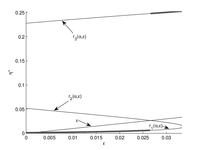
Analytical expressions for the $r_{i}(\alpha,\varepsilon)$ and $\tau_{i}(\alpha)$ are determined for the (3,6) regular LDPC code by solving the appropriate polynomial equations and numerical evaluations of the $r_{i}$ expressions are shown as thin lines in Fig. 4 as functions of $\varepsilon$ for fixed $\alpha$ . The point where $r_{1}(\alpha,\varepsilon)=\varepsilon$ is $\tau_{1}(\alpha)$ and the point where $r_{2}(\alpha,\varepsilon)=\varepsilon$ is $\tau_{2}(\alpha)$ . In Fig. 4, these are points where the thin lines cross.

By analyzing the dynamical system equation (1) for the (3,6) code in detail, it can be shown that $r_{1}(\alpha,\varepsilon)$ and $r_{3}(\alpha,\varepsilon)$ are stable fixed points of density evolution. Contrarily, $r_{2}(\alpha,\varepsilon)$ is an unstable fixed point, which determines the boundary between the regions of attraction for the two stable fixed points. Since $r_{1}(\alpha,\varepsilon)$ and $r_{3}(\alpha,\varepsilon)$ are stable fixed points, the final error probability $\eta^{*}$ will take on one of these two values, depending on the starting point of the recursion, $\varepsilon$ . The thick line in Fig. 4 shows the final error probability $\eta^{*}$ as a function of initial error probability $\varepsilon$ . One may note that $\eta^{*}=r_{1}$ is the desirable small error probability, whereas $\eta^{*}=r_{3}$ is the undesirable large error probability and that $\tau_{2}$ delimits these two regimes.

The $\tau(\alpha)$ points determine when it is beneficial to use the decoder, in the sense that $\eta^{*}<\varepsilon$ . By varying $\alpha$ (as if in a sequence of plots like Fig. 4), an $\alpha-\varepsilon$ region where the decoder is beneficial is demarcated; this is shown in Fig. 5. The function $\tau_{2}(\alpha)$ is the $\eta$ -reliability decoding threshold for large ranges of $\eta$ .

Notice that the previously known special case, the decoding threshold of the noiseless decoder, can be recovered from these results. The decoding threshold for the noiseless decoder is denoted $\varepsilon^{*}_{BRU}$ and is equal to the following expression [74].

\varepsilon^{*}_{BRU}=\frac{1-\sqrt{\sigma}}{2}\mbox{,}

where

\sigma=-\frac{1}{4}+\frac{\sqrt{-\tfrac{5}{12}-b}}{2}+\frac{\sqrt{-\tfrac{5}{6}+\tfrac{11}{4\sqrt{-5/12-b}}}}{2}

and

b=\frac{8}{3}\left(\frac{2}{83+3\sqrt{993}}\right)^{\tfrac{1}{3}}-\frac{1}{3}\left(\frac{83+3\sqrt{993}}{2}\right)^{\tfrac{1}{3}}\mbox{.}

This value is recovered from noisy decoder results by noting that $\eta^{*}(\alpha=0,\varepsilon)=0$ for $\varepsilon\in\left[0,\varepsilon^{*}_{BRU}\right]$ , which are the ordinate intercepts of the region in Fig. 5.

To provide a better sense of the performance of the noisy Gallager A algorithm, Table I lists some values of $\alpha$ , $\varepsilon$ , and $\eta^{*}$ (numerical evaluations are listed and an example of an analytical expression is given in Appendix C). As can be seen from these results, particularly from the $\tau_{2}$ curve in Fig. 5, the error probability performance of the system degrades gracefully as noise is added to the decoder.

TABLE I: Performance of Noisy Gallager A algorithm for (3,6) code

$\alpha$	$\varepsilon^{*}(0.1,\alpha)$	$\eta^{}(\alpha,\varepsilon^{})$	$\eta^{*}(\alpha,0.01)$
$0$	$0.0394636562$	$0$	$0$
$1\times 10^{-10}$	$0.0394636560$	$7.8228\times 10^{-11}$	$1.3333\times 10^{-11}$
$1\times 10^{-8}$	$0.0394636335$	$7.8228\times 10^{-9}$	$1.3333\times 10^{-9}$
$1\times 10^{-6}$	$0.0394613836$	$7.8234\times 10^{-7}$	$1.3338\times 10^{-7}$
$1\times 10^{-4}$	$0.0392359948$	$7.8866\times 10^{-5}$	$1.3812\times 10^{-5}$
$3\times 10^{-4}$	$0.0387781564$	$2.4050\times 10^{-4}$	$4.4357\times 10^{-5}$
$1\times 10^{-3}$	$0.0371477336$	$8.4989\times 10^{-4}$	$1.8392\times 10^{-4}$
$3\times 10^{-3}$	$0.0321984070$	$3.0536\times 10^{-3}$	$9.2572\times 10^{-4}$
$5\times 10^{-3}$	$0.0266099758$	$6.3032\times 10^{-3}$	$2.4230\times 10^{-3}$

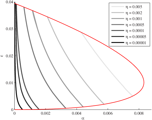
Returning to threshold characterization, an analytical expression for the threshold within the region to use decoder is:

\varepsilon^{*}(\eta,\alpha)=\frac{\eta-q_{\alpha}^{-}(\eta)}{1-q_{\alpha}^{+}(\eta)-q_{\alpha}^{-}(\eta)}\mbox{,}

which is the solution to the polynomial equation in $\check{\epsilon}$ ,

\check{\epsilon}-\check{\epsilon}q_{\alpha}^{+}(\eta)+(1-\check{\epsilon})q_{\alpha}^{-}(\eta)-\eta=0\mbox{.}

The threshold is drawn for several values of $\eta$ in Fig. 6. A threshold line determines the equivalence of channel noise and decoder noise with respect to final probability of error. If for example, the binary symmetric channels in the system are a result of hard-detected AWGN channels, such a line may be used to derive the equivalent channel noise power for decoder noise power or vice versa. Threshold lines therefore provide guidelines for power allocation in communication systems.

V-C Code Optimization

At this point, the bit error performance of a system has simply been measured; no attempt has been made to optimize a code for a particular decoder and set of parameters. For fault-free decoding, it has been demonstrated that irregular code ensembles can perform much better than regular code ensembles like the (3,6) LDPC considered above [77, 74]. One might hope for similar improvements when LDPC code design takes decoder noise into account. The space of system parameters to be considered for noisy decoders is much larger than for noiseless decoders.

As a first step, consider the ensemble of rate $1/2$ LDPC codes that were optimized by Bazzi et al. for the fault-free Gallager A decoding algorithm [74]. The left degree distribution is

\lambda(\zeta)=a\zeta^{2}+(1-a)\zeta^{3}

and the right degree distribution is

\rho(\zeta)=\frac{7a}{3}\zeta^{6}+\frac{3-7a}{3}\zeta^{7}\mbox{,}

where the optimal $a$ is specified analytically. Numerically, $a_{\text{opt}}=0.1115\ldots$ . Measuring the performance of this code with the noisy Gallager A decoder yields the region to use decoder shown in Fig. 7; the region to use decoder for the (3,6) code is shown for comparison. By essentially any criterion of performance, this optimized code is better than the (3,6) code.

Are there other codes that can perform better on the faulty decoder than the code optimized for the fault-free decoder? To see whether this is possible, arbitrarily restrict to the family of ensembles that were found to contain the optimal degree distribution for the fault-free decoder and take $a=1/10$ . Also let $\alpha=1/500$ be fixed. The numerical value of the threshold $\varepsilon_{1/10}^{*}(1/10,\alpha)=0.048239$ , whereas the numerical value of the threshold $\varepsilon_{a_{\text{opt}}}^{*}(1/10,\alpha)=0.047857$ . In this sense, the $a=1/10$ code is better than the $a=a_{\text{opt}}$ code. In fact, as seen in Fig. 7, the region to use decoder for this $a=1/10$ code contains the region to use decoder for the $a_{\text{opt}}$ code.

On the other hand, the final error probability when operating at threshold for the $a=1/10$ code $\eta_{1/10}^{*}(\alpha,\varepsilon_{1/10}^{*}(1/10,\alpha))=0.01869$ , whereas the final error probability when operating at threshold for the $a=a_{\text{opt}}$ code is $\eta_{a_{\text{opt}}}^{*}(\alpha,\varepsilon_{a_{\text{opt}}}^{*}(1/10,\alpha))=0.01766$ . So in this sense, the $a=a_{\text{opt}}$ code is better than the $a=1/10$ code. The fact that highly optimized ensembles usually lead to more simultaneous critical points is the main complication.

If both threshold and final bit error probability are performance criteria, there is no total order on codes and therefore there may be no notion of an optimal code.

VI Example: Noisy Gaussian Decoder

It is also of interest to analyze a noisy version of the belief propagation decoder applied to the output of a continuous-alphabet channel. Density evolution for belief propagation is difficult to analyze even in the noiseless decoder case, and so a Gaussian approximation method [78] is used. The state variables are one-dimensional rather than infinite-dimensional as for full analysis of belief propagation. The specific node computations carried out by the decoder are as in belief propagation [13]; these can be approximated by the functions $\Phi$ and $\Psi$ defined below. The messages and noise model are specified in terms of the approximation.

Section V had considered decoding the output of a BSC with a decoder that was constructed with BSC components and Proposition 1 had shown that probability of bit error could never be driven to zero. Here, the probability of bit error does in fact go to zero.

Consider a binary input AWGN channel with variance $\varepsilon^{2}$ . The output is decoded using a noisy Gaussian decoder. For simplicity, only regular LDPC codes are considered. The messages that are passed in this decoder are real-valued, $\mathcal{M}=\mathbb{R}\cup\{\pm\infty\}$ , and are in belief format.

The variable-to-check messages in the zeroth iteration are the log-likelihood ratios computed from the channel output symbols, $\nu(y)$ ,

\nu_{\tt{v}\to\tt{c}}=\nu(y)=\log\frac{p(y|x=1)}{p(y|x=-1)}\mbox{.}

The check node takes the received versions of these messages, $\mu_{\tt{v}\to\tt{c}}$ , as input. The node implements a mapping $\Phi$ whose output, $\nu_{\tt{c}\to\tt{v}}$ , satisfies:

\operatorname{etanh}(\nu_{\tt{c}\to\tt{v}})=\prod_{i=1}^{{d_{\tt{c}}}-1}\operatorname{etanh}(\mu_{{\tt{v}\to\tt{c}}_{i}})\mbox{,}

where the product is taken over messages on all incoming edges except the one on which the message will be outgoing, and

\operatorname{etanh}(\check{v})=\frac{1}{\sqrt{4\pi\check{v}}}\int_{\mathbb{R}}\tanh\frac{v}{2}e^{-\frac{(v-\check{v})^{2}}{4v}}dv\mbox{.}

The check node mapping is motivated by Gaussian likelihood computations. For the sequel, it is useful to define a slightly different function

\phi(\check{v})=\begin{cases}1-\operatorname{etanh}(\check{v})\mbox{,}&\check{v}>0\\ 1\mbox{,}&\check{v}=0\end{cases}

which can be approximated as

\phi(\check{v})\approx e^{a\check{v}^{c}+b}\mbox{,}

with $a=-0.4527$ , $b=0.0218$ , $c=0.86$ [78].

For iterations $\ell\geq 1$ , the variable node takes the received versions of the $\tt{c}\to\tt{v}$ messages, $\mu_{\tt{c}\to\tt{v}}$ , as inputs. The mapping $\Psi$ yields output $\nu_{\tt{v}\to\tt{c}}$ given by

\nu_{\tt{v}\to\tt{c}}=\nu(y)+\sum_{i=1}^{{d_{\tt{v}}}-1}\mu_{{\tt{c}\to\tt{v}}_{i}}\mbox{,}

where the sum is taken over received messages from the neighboring check nodes except the one to which this message is outgoing. Again, the operation of the variable node is motivated by Gaussian likelihood computations.

As in Section V, local computation noise is combined into message-passing noise (Fig. 3). To model quantization [25] or random phenomena, consider each message passed in the decoder to be corrupted by signal-independent additive noise which is bounded as $-\alpha/2\leq w\leq\alpha/2$ . This class of noise models includes uniform noise, and truncated Gaussian noise, among others. If the noise is symmetric, then Theorem 1 applies. Following the von Neumann error model, each noise realization $w$ is assumed to be independent.

VI-A Density Evolution Equation

The definition of the computation rules and the noise model may be used to derive the approximate density evolution equation. The one-dimensional state variable chosen to be tracked is $s$ , the mean belief at a variable node. The symmetry condition relating mean belief to belief variance [13, 78] is enforced. Thus, if the all-one codeword was transmitted, then the value $s$ going to $+\infty$ implies that the density of $\nu_{\tt{v}\to\tt{c}}$ tends to a “mass point at infinity,” which in turn implies that $P_{e}$ goes to $0$ .

To bound decoding performance under any noise model in the class of additive bounded noise, consider (non-stochastic) worst-case noise. Assuming that the all-one codeword was sent, all messages should be as positive as possible to move towards the correct decoded codeword (mean beliefs of $+\infty$ indicate perfect confidence in a bit being $1$ ). Consequently, the worst bounded noise that may be imposed is to subtract $\alpha/2$ from all messages that are passed; this requires knowledge of the transmitted codeword being all-one. If another codeword is transmitted, then certain messages would have $\alpha/2$ added instead of subtracted.

Such a worst-case noise model does not meet the conditions of Theorem 1, but transmission of the all-one codeword is assumed nonetheless. If there were an adversary with knowledge of the transmitted codeword imposing worst-case noise on the decoder, then probability of bit error would be conditionally independent of the transmitted codeword, as given in Appendix A-1.

Note that the adversary is restricted to selecting each noise realization independently. More complicated and devious error patterns in space or in time are not possible in the von Neumann error model. Moreover, the performance criterion is probability of bit error rather than probability of block error, so complicated error patterns would provide no great benefit to the adversary.

Since the noise is conditionally deterministic given the transmitted codeword, derivation of the density evolution equation is much simplified. An induction argument is used, and the base case is

s_{0}=\tfrac{2}{\varepsilon^{2}}\mbox{,}

where $\varepsilon^{2}$ is the channel noise power. This follows from the log-likelihood computation for an AWGN communication channel with input alphabet $\mathcal{X}=\{\pm 1\}$ .

The inductive assumption in the induction argument is $s_{\ell-1}$ . This message is communicated over message-passing noise to get

s_{\ell-1}-\tfrac{\alpha}{2}\mbox{.}

Next the check node computation is made to yield

\phi^{-1}\left(1-[1-\phi(s_{\ell-1}-\tfrac{\alpha}{2})]^{{d_{\tt{c}}}-1}\right)\mbox{.}

By the inductive assumption, all messages will be equivalent; that is why the product is a $({d_{\tt{c}}}-1)$ -fold product of the same quantity. This value is communicated over message-passing noise to get

\phi^{-1}\left(1-[1-\phi(s_{\ell-1}-\tfrac{\alpha}{2})]^{{d_{\tt{c}}}-1}\right)-\tfrac{\alpha}{2}\mbox{.}

Finally the variable-node computation yields

s_{0}+({d_{\tt{v}}}-1)\left\{\phi^{-1}\left(1-[1-\phi(s_{\ell-1}-\tfrac{\alpha}{2})]^{{d_{\tt{c}}}-1}\right)-\tfrac{\alpha}{2}\right\}\mbox{.}

Again, all messages will be equivalent so the sum is a $({d_{\tt{v}}}-1)$ -fold sum of the same quantity. Thus the density evolution equation is

s_{\ell}=\tfrac{2}{\varepsilon^{2}}-\tfrac{({d_{\tt{v}}}-1)\alpha}{2}+({d_{\tt{v}}}-1)\left\{\phi^{-1}\left(1-[1-\phi(s_{\ell-1}-\tfrac{\alpha}{2})]^{{d_{\tt{c}}}-1}\right)\right\}\mbox{.}

(4)

VI-B Performance Evaluation

One might wonder whether there are sets of noise parameters $\alpha>0$ and $\varepsilon>0$ such that $s_{\ell}\to+\infty$ . Indeed there are, and there is a threshold phenomenon just like Chung et al. showed for $\alpha=0$ [78].

Proposition 2

Final error probability $\eta^{*}=0$ for LDPC ensembles decoded using the noisy Gaussian system defined in Section VI, for binary-input AWGN channels with noise level $\varepsilon<\varepsilon^{*}(\alpha)$ .

Proof:

Substituting $s=+\infty$ into (4) demonstrates that it is a stable fixed point. It may further be verified that the dynamical system proceeds toward that fixed point if $\varepsilon<\varepsilon^{*}(\alpha)$ . ∎Unlike Section V where the $\varepsilon^{*}(\eta,\alpha)$ thresholds could be evaluated analytically, only numerical evaluations of these $\varepsilon^{*}(\alpha)$ thresholds are possible. These are shown in Fig. 8 for three regular LDPC ensembles with rate $1/2$ , namely the (3,6) ensemble, the (4,8) ensemble, and the (5,10) ensemble. As can be observed, thresholds decrease smoothly as the decoder noise level increases. Moreover, the ordering of the codes remains the same for all levels of decoder noise depicted. Code optimization remains to be done.

The basic reason for the disparity between Propositions 2 and 1 is that here, the noise is bounded whereas the messages are unbounded. Thus once the messages grow large, the noise has essentially no effect. To use a term from [67], once the decoder reaches the breakout value, noise cannot stop the decoder from achieving Shannon reliability.

Perhaps a peak amplitude constraint on messages would provide a more realistic computation model, but the equivalent of Proposition 2 may not hold. Quantified data processing inequalities may provide insight into what forms of noise and message constraints are truly limiting [35, 34].

VII Application: Reliable Memories Constructed from Unreliable Components

In Section I, complexity and reliability were cast as the primary limitations on practical decoding. By considering the design of fault masking techniques for memory systems, a communication problem beyond Fig. 1, both complexity and reliability may be explicitly constrained. Indeed, the problem of constructing reliable information storage devices from unreliable components is central to fault-tolerant computing, and determining the information storage capacity of such devices is a long-standing open problem [79]. This problem is related to problems in distributed information storage [80] and is intimately tied to the performance of codes under faulty decoding. The analysis techniques developed thus far may be used directly.

In particular, one may construct a memory architecture with noisy registers and a noisy LDPC correcting network. At each time step, the correcting network decodes the register contents and restores them. The correcting network prevents the codeword stored in the registers from wandering too far away. Taylor and others have shown that there exist non-zero levels of component noisiness such that the LDPC-based construction achieves non-zero storage capacity [54, 55, 63]. Results as in Section V may be used to precisely characterize storage capacity.

Before proceeding with an achievability result, requisite definitions and the problem statement are given [54].

Definition 6

An elementary operation is any Boolean function of two binary operands.

Definition 7

A system is considered to be constructed from components, which are devices that either perform one elementary operation or store one bit.

Definition 8

The complexity $\chi$ of a system is the number of components within the system.

Definition 9

A memory system that stores $k$ information bits is said to have an information storage capability of $k$ .

Definition 10

Consider a sequence of memories $\{M_{i}\}$ , ordered according to their information storage capability $i$ (bits). The sequence $\{M_{i}\}$ is stable if it satisfies the following:

1.

For any $k$ , $M_{k}$ must have $2^{k}$ allowed inputs denoted $\{I_{k_{i}}\}$ , $1\leq i\leq 2^{k}$ .
2.

A class of states, $C(I_{k_{i}})$ , is associated with each input $I_{k_{i}}$ of $M_{k}$ . The classes $C(I_{k_{i}})$ and $C(I_{k_{j}})$ must be disjoint for all $i\neq j$ and all $k$ .
3.

The complexity of $M_{k}$ , $\chi(M_{k})$ , must be bounded by $\theta k$ , where redundancy $\theta$ is fixed for all $k$ .
4.

At $\ell=0$ , let one of the inputs from $\{I_{k_{i}}\}$ be stored in each memory $M_{k}$ in the sequence of memories $\{M_{i}\}$ , with no further inputs in times $\ell>0$ . Let $I_{k_{i}}$ denote the particular input stored in memory $M_{k}$ . Let $\lambda_{k_{i}}(T)$ denote the probability that the state of $M_{k}$ does not belong to $C(I_{k_{i}})$ at $\ell=T$ and further let $P^{\max}_{k}(T)=\max_{i}\lambda_{k_{i}}(T)$ . Then for any $T>0$ and $\delta>0$ , there must exist a $k$ such that $P^{\max}_{k}(T)<\delta$ .

The demarcation of classes of states is equivalent to demarcating decoding regions.

Definition 11

The storage capacity, $\mathfrak{C}$ , of memory is a number such that there exist stable memory sequences for all memory redundancy values $\theta$ greater than $1/\mathfrak{C}$ .

Note that unlike channel capacity for the communication problem, there is no informational definition of storage capacity that is known to go with the operational definition.

The basic problem then is to determine storage capacity, which is a measure of the circuit complexity required to achieve arbitrarily reliable information storage. The circuit complexity must be linear in blocklength, a property satisfied by systems with message-passing correcting networks for LDPC codes.

Although Proposition 1 shows that Shannon reliability is not achievable for any noisy Gallager A decoder, the definition of stable information storage does not require this. By only requiring maintenance within a decoding region, the definition implies that either the contents of the memory may be read-out in coded form or equivalently that there is a noiseless output device that yields decoded information; call this noiseless output device the silver decoder.

Consider the construction of a memory with noisy registers as storage elements. These registers are connected to a noisy Gallager A LDPC decoder (as described in Section V), which takes the register values as inputs and stores its computational results back into the registers. To find the storage capacity of this construction, first compute the complexity (presupposing that the construction will yield a stable sequence of memories).

The Gallager A check node operation is a $({d_{\tt{c}}}-1)$ -input XOR gate, which may be constructed from ${d_{\tt{c}}}-2$ two-input XOR gates. A variable node determines whether its ${d_{\tt{v}}}-1$ inputs are all the same and then compares to the original received value. Let $D_{{d_{\tt{v}}}}$ denote the complexity of this logic. The output of the comparison to the original received value is the value of the consensus view. One construction to implement the consensus logic is to OR together the outputs of a $({d_{\tt{v}}}-1)$ -input AND gate and a $({d_{\tt{v}}}-1)$ -input AND gate with inverted inputs. This is then XORed with the stored value. Such a circuit can be implemented with $2({d_{\tt{v}}}-2)+2$ components, so $D_{{d_{\tt{v}}}}=2{d_{\tt{v}}}-2$ . The storage is carried out in $n$ registers. The total complexity of the memory $M_{k}$ , $\chi(M_{k})_{\mathcal{C}^{n}({d_{\tt{v}}},{d_{\tt{c}}})}$ , is

\chi(M_{k})_{\mathcal{C}^{n}({d_{\tt{v}}},{d_{\tt{c}}})}=n(1+2{d_{\tt{v}}}-2+{d_{\tt{v}}}({d_{\tt{c}}}-2))=n({d_{\tt{v}}}{d_{\tt{c}}}-1)\mbox{.}

The information storage capability is $n$ times the rate of the code, $R$ . The complexity of an irredundant memory with the same storage capability is $\chi_{\mbox{irr}_{n}}=Rn$ . Hence, the redundancy is

\frac{\chi(M_{k})_{\mathcal{C}^{n}({d_{\tt{v}}},{d_{\tt{c}}})}}{\chi_{\mbox{irr}_{n}}}=\frac{n({d_{\tt{v}}}{d_{\tt{c}}}-1)}{Rn}\leq\frac{({d_{\tt{v}}}{d_{\tt{c}}}-1)}{1-{d_{\tt{v}}}/{d_{\tt{c}}}}

which is a constant. By [65, Lemma 3.22], the inequality almost holds with equality with high probability for large $n$ . For the $(3,6)$ regular LDPC code, the redundancy value is $34$ , so $\mathfrak{C}=1/34$ , if the construction does in fact yield stable memories.

The conditions under which the memory is stable depends on the silver decoder. Since silver decoder complexity does not enter, maximum likelihood should be used. The Gallager lower bound to the ML decoding threshold for the $(3,6)$ regular LDPC code is $\varepsilon^{*}_{GLB}=0.0914755$ [81, Table II]. Recall from Fig. 5 that the decoding threshold for Gallager A decoding is $\varepsilon^{*}_{BRU}=0.0394636562$ .

If the probability of bit error for the correcting network in the memory stays within the decoding threshold of the silver decoder, then stability follows. Thus the question reduces to determining the sets of component noisiness levels $(\alpha,\varepsilon)$ for which the decoding circuit achieves $(\eta=\varepsilon^{*}_{ML})$ -reliability.

Consider a memory system where bits are stored in registers with probability $\alpha_{r}$ of flipping at each time step. An LDPC codeword is stored in these registers; the probability of incorrect storage at the first time step is $\varepsilon$ . At each iteration, the variable node value from the correcting network is placed in the register. This stored value is used in the subsequent Gallager A variable node computation rather than a received value from the input pins. Suppose that the component noise values in the correcting network may be parameterized as in Section V. Then a slight modification of the analysis in Section V yields a density evolution equation

s_{\ell+1}=\varepsilon_{2}-\varepsilon_{2}q_{\alpha}^{+}(s_{\ell})+(1-\varepsilon_{2})q_{\alpha}^{-}(s_{\ell})\mbox{,}

where $\varepsilon_{2}=s_{\ell}(1-\alpha_{r})+\alpha_{r}(1-s_{\ell})$ . There is a “region to use decoder” for this system, just as in Section V. If $\alpha_{r}=\alpha$ , this region is shown in Fig. 9, and is slightly smaller than the region in Fig. 5. Denote this region and its hypograph as $\mathfrak{R}$ . It follows that $(\eta=\varepsilon^{*}_{BRU})$ -reliability is achieved for $\mathfrak{R}$ . Since $\varepsilon^{*}_{BRU}$ -reliability is achievable, $\varepsilon^{*}_{GLB}$ -reliability is achievable by monotonicity. Thus the construction yields stable memories.

Proposition 3

Let $\mathfrak{R}$ be the set of memory component noise parameters $(\alpha,\varepsilon)$ within the region to use decoder or its hypograph corresponding to a system with a Gallager A correcting network for the $(3,6)$ LDPC code, depicted in Fig. 9. Then a sequence of memories constructed from $\mathfrak{R}$ -components have a storage capacity lower bounded as $\mathfrak{C}\geq 1/34$ .

This may be directly generalized for any choice of code ensemble as follows.

Theorem 5

Let $\mathfrak{R}$ be the (computable) set of memory component noise parameters $(\alpha,\varepsilon)$ within the region to use decoder or its hypograph corresponding to a system with a Gallager A correcting network for the $(\lambda,\rho)$ LDPC code. Then a sequence of memories constructed from $\mathfrak{R}$ -components have a storage capacity lower bounded as

\mathfrak{C}\geq\frac{1-\lambda^{\prime}(1)/\rho^{\prime}(1)}{\lambda^{\prime}(1)\rho^{\prime}(1)-1}\mbox{.}

The bound reduces to $({1-{d_{\tt{v}}}/{d_{\tt{c}}}})/({{d_{\tt{v}}}{d_{\tt{c}}}-1})$ for regular codes.

This theorem gives a precise achievability result that bounds storage capacity. It also implies a code ensemble optimization problem similar to the one in Section V-C. The question of an optimal architecture for memory systems however remains open.

VIII Conclusions

Loeliger et al. [7] had observed that decoders are robust to nonidealities and noise in physical implementations, however they had noted that “the quantitative analysis of these effects is a challenging theoretical problem.” This work has taken steps to address this challenge by characterizing robustness to decoder noise.

The extension of the density evolution method to the case of faulty decoders allows a simplified means of asymptotic performance characterization. Results from this method show that in certain cases Shannon reliability is not achievable (Proposition 1), whereas in other cases it is achievable (Proposition 2). In either case, however, the degradation of a suitably defined decoding threshold is smooth with increasing decoder noise, whether in circuit nodes or circuit wires. Due to this smoothness, codes optimized for fault-free decoders do work well with faulty decoders, however optimization of codes for systems with faulty decoders remains to be studied.

No attempt was made to apply fault masking methods to develop decoding algorithms with improved performance in the presence of noise. One approach might be to use coding within the decoder so as to reduce the values of $\alpha$ . Of course, the within-decoder code would need to be decoded. There are also more direct circuit-oriented techniques that may be applied [82, 83]. Following the concept of concatenated codes, concatenated decoders may also be promising. The basic idea of using a first (noiseless) decoder to correct many errors and then a second (noiseless) decoder to clean things up was already present in [61], but it may be extended to the faulty decoder setting.

Reducing power consumption in decoder circuits has been an active area of research [84, 85, 86, 37, 87, 88, 89, 90], however power reduction often has the effect of increasing noise in the decoder [91]. The tradeoff developed between the quality of the communication channel and the quality of the decoder may provide guidelines for allocating resources in communication system design.

Analysis of other decoding algorithms with other error models will presumably yield results similar to those obtained here. For greater generality, one might move beyond simple LDPC codes and consider arbitrary codes decoded with very general iterative decoding circuits [90] with suitable error models. An even more general model of computation such as a Turing machine or beyond [92] does not seem to have an obvious, appropriate error model.

Even just a bit of imagination provides numerous models of channel noise and circuit faults that may be investigated in the future to provide further insights into the fundamental limits of noisy communication and computing.

Acknowledgment

I thank Rüdiger L. Urbanke and İ. Emre Telatar for several enlightening discussions, for encouragement, and for hosting my visit at EPFL. I also thank the anonymous reviewers, Sanjoy K. Mitter, G. David Forney, and Vivek K Goyal for assistance in improving the paper. Thanks also to Shashi Kiran Chilappagari for telling me about his work.

Appendix A Proof of Theorem 1

Let ${\bf x}\in\mathcal{C}^{n}$ be a codeword and let $\bf{Y}$ denote the corresponding channel output $\bf{Y}=\bf{x}\bf{Z}$ (where the notation means pointwise multiplication on length $n$ vectors). Note that $\bf{Z}$ is equal to the channel output observation when $\bf{x}$ is all-one. The goal is to show that messages sent during the decoding process for cases when the received codeword is either $\bf{x}\bf{Z}$ or $\bf{x}$ correspond.

Let $\dot{n}_{i}$ be an arbitrary variable node and let $\dot{n}_{j}$ be one of its neighboring check nodes. Let $\nu_{ij}^{(\ell)}(\bf{y})$ and $\mu_{ij}^{(\ell)}(\bf{y})$ denote the variable-to-check message from $\dot{n}_{i}$ to $\dot{n}_{j}$ at the respective terminals in iteration $\ell$ , assuming received value $\bf{y}$ . Similarly, let $\nu_{ji}^{(\ell)}(\bf{y})$ and $\mu_{ji}^{(\ell)}(\bf{y})$ be the check-to-variable message from $\dot{n}_{j}$ to $\dot{n}_{i}$ at the respective terminal in iteration $\ell$ assuming received value $\bf{y}$ .

By Definition 2, the channel is memoryless binary-input output-symmetric and it may be modeled multiplicatively as

Y_{t}=x_{t}Z_{t}\mbox{,}

(5)

where $\{Z_{t}\}$ is a sequence of i.i.d. random variables and $t$ is the channel usage time. The validity of the multiplicative model is shown in [13, p. 605] and [65, p. 184].

The proof proceeds by induction and so the base case is established first. By the multiplicative model (5), $\nu_{ij}^{(0)}({\bf y})=\nu_{ij}^{(0)}({\bf xz})$ . Recalling that $x_{i}\in\{\pm 1\}$ , by the variable node symmetry condition (Definition $3$ ) which includes computation noise $u_{\dot{n}_{i}}^{(0)}$ , it follows that $\nu_{ij}^{(0)}({\bf y})=\nu_{ij}^{(0)}({\bf xz})=x_{i}\nu_{ij}^{(0)}({\bf z})$ .

Now take the wire noise $w_{ij}^{(0)}$ on the message from $\dot{n}_{i}$ to $\dot{n}_{j}$ into account. It is symmetric (Definition 5) and so $\nu_{ij}^{(0)}({\bf y})=x_{i}\nu_{ij}^{(0)}({\bf z})$ implies a similar property for $\mu_{ij}^{(0)}$ . In particular,

$\displaystyle\mu_{ij}^{(0)}({\bf y})$	$\displaystyle=\Xi(\nu_{ij}^{(0)}({\bf y}),w_{ij}^{(0)})$	(6)
	$\displaystyle=\Xi(x_{i}\nu_{ij}^{(0)}({\bf z}),w_{ij}^{(0)})$
	$\displaystyle=x_{i}\Xi(\nu_{ij}^{(0)}({\bf z}),x_{i}w_{ij}^{(0)})$

where the last step follows because $x_{i}\in\{\pm 1\}$ and so it can be taken outside of $\Xi$ by Definition 5, when it is put back in for the wire noise. Now since $x_{i}\in\{\pm 1\}$ and since the wire noise is symmetric about $0$ by Definition 5, $x_{i}\Xi(\nu_{ij}^{(0)}({\bf z}),x_{i}w_{ij}^{(0)})$ will correspond to $x_{i}\mu_{ij}^{(0)}({\bf z})$ , in the sense that error event probabilities will be identical.

Assume that $\mu_{ij}^{(\ell)}({\bf y})$ corresponds to $x_{i}\mu_{ij}^{(\ell)}({\bf z})$ for all $(i,j)$ pairs and some $\ell\geq 0$ as the inductive assumption. Let $\mathcal{N}_{\dot{n}_{j}}$ be the set of all variable nodes that are connected to check node $\dot{n}_{j}$ . Since $\bf{x}$ is a codeword, it satisfies the parity checks, and so $\prod_{k\in\mathcal{N}_{\dot{n}_{j}}}=1$ . Then from the check node symmetry condition (Definition 3), $\nu_{ji}^{(\ell+1)}({\bf y})$ corresponds to $x_{i}\nu_{ji}^{(\ell+1)}({\bf z})$ . Further, by the wire noise symmetry condition (Definition 5) and the same argument as for the base case, $\mu_{ji}^{(\ell+1)}({\bf y})$ corresponds to $x_{i}\mu_{ji}^{(\ell+1)}({\bf z})$ . By invoking the variable node symmetry condition (Definition 4) again, it follows that $\nu_{ij}^{(\ell+1)}({\bf y})$ corresponds to $x_{i}\nu_{ij}^{(\ell+1)}({\bf z})$ for all $(i,j)$ pairs.

Thus by induction, all messages to and from variable node $\dot{n}_{i}$ when $\bf{y}$ is received correspond to the product of $x_{i}$ and the corresponding message when $\bf{z}$ is received.

Both decoders proceed in correspondence and commit exactly the same number of errors.

A-1 Worst-Case Noise

The same result with the same basic proof also holds when the wire noise operation $\Xi$ is symmetric but $w$ is not symmetric stochastic, but is instead worst-case. The only essential modification is in (6) and the related part of the induction step. Since wire noise is dependent on $x_{i}$ , it can be written as $x_{i}w$ . Thus,

	$\displaystyle\mu_{ij}^{(0)}({\bf y})$	$\displaystyle=\Xi(\nu_{ij}^{(0)}({\bf y}),x_{i}w_{ij}^{(0)})$
		$\displaystyle=\Xi(x_{i}\nu_{ij}^{(0)}({\bf z}),x_{i}w_{ij}^{(0)})$
		$\displaystyle\stackrel{{\scriptstyle(a)}}{{=}}x_{i}\Xi(\nu_{ij}^{(0)}({\bf z}),w_{ij}^{(0)})$
		$\displaystyle=x_{i}\mu_{ij}^{(0)}({\bf z})$

where step (a) follows because $x_{i}\in\{\pm 1\}$ and so it can be taken outside of $\Xi$ by the symmetry property of $\Xi$ . Thus the two decoders will proceed in exact one-to-one correspondence, not just in probabilistic correspondence.

Appendix B Proof of Theorem 2

Prior to giving the proof of Theorem 2, a review of some definitions from probability theory [93] and the Hoeffding-Azuma inequality are provided.

Consider a measurable space $(\Omega,\mathcal{F})$ consisting of a sample space $\Omega$ and a $\sigma$ -algebra $\mathcal{F}$ of subsets of $\Omega$ that contains the whole space and is closed under complementation and countable unions. A random variable is an $\mathcal{F}$ -measurable function on $\Omega$ . If there is a collection $(Z_{\gamma}|\gamma\in C)$ of random variables $Z_{\gamma}:\Omega\to\mathbb{R}$ , then

\mathcal{Z}=\sigma(Z_{\gamma}|\gamma\in C)

is defined to be the smallest $\sigma$ -algebra $\mathcal{Z}$ on $\Omega$ such that each map $(Z_{\gamma}|\gamma\in C)$ is $\mathcal{Z}$ -measurable.

Definition 12 (Filtration)

Let $\{\mathcal{F}_{i}\}$ be a sequence of $\sigma$ -algebras with respect to the same sample space $\Omega$ . These $\mathcal{F}_{i}$ are said to form a filtration if $\mathcal{F}_{0}\subseteq\mathcal{F}_{1}\subseteq\cdots$ are ordered by refinement in the sense that each subset of $\Omega$ in $\mathcal{F}_{i}$ is also in $\mathcal{F}_{j}$ for $i\leq j$ . Also $\mathcal{F}_{0}=\{\emptyset,\Omega\}$ .

Usually, $\{\mathcal{F}_{i}\}$ is the natural filtration $\mathcal{F}_{i}=\sigma(Z_{0},Z_{1},\ldots,Z_{i})$ of some sequence of random variables $(Z_{0},Z_{1},\ldots)$ , and then the knowledge about $\omega$ known at step $i$ consists of the values $Z_{0}(\omega),Z_{1}(\omega),\ldots,Z_{i}(\omega)$ .

For a probability triple $(\Omega,\mathcal{F},\mathbb{P})$ , a version of the conditional expectation of a random variable $Z$ given a $\sigma$ -algebra $\mathcal{F}$ is a random variable denoted $E\left[{Z|\mathcal{F}}\right]$ . Two versions of conditional expectation agree almost surely, but measure zero departures are not considered subsequently; one version is fixed as canonical. Conditional expectation given a measurable event $\mathfrak{E}$ is denoted $E\left[{Z|\sigma(\mathfrak{E})}\right]$ and conditional expectation given a random variable $W$ is denoted $E\left[{Z|\sigma(W)}\right]$ .

Definition 13 (Martingale)

Let $\mathcal{F}_{0}\subseteq\mathcal{F}_{1}\subseteq\cdots$ be a filtration on $\Omega$ and let $Z_{0},Z_{1},\ldots$ be a sequence of random variables on $\Omega$ such that $Z_{i}$ is $\mathcal{F}_{i}$ -measurable. Then $Z_{0},Z_{1},\ldots$ is a martingale with respect to the filtration $\mathcal{F}_{0}\subseteq\mathcal{F}_{1}\subseteq\cdots$ if $E\left[{Z_{i}|\mathcal{F}_{i-1}}\right]=Z_{i-1}$ .

A generic way to construct a martingale is Doob’s construction.

Definition 14 (Doob Martingale)

Let $\mathcal{F}_{0}\subseteq\mathcal{F}_{1}\subseteq\cdots$ be a filtration on $\Omega$ and let $Z$ be a random variable on $\Omega$ . Then the sequence of random variables $Z_{0},Z_{1},\ldots$ such that $Z_{i}=E\left[{Z|\mathcal{F}_{i}}\right]$ is a Doob martingale.

Lemma 1 (Hoeffding-Azuma Inequality [94, 95, 13])

Let $Z_{0},Z_{1},\ldots$ be a martingale with respect to the filtration $\mathcal{F}_{0}\subseteq\mathcal{F}_{1}\subseteq\cdots$ such that for each $i>0$ , the following bounded difference condition is satisfied

|Z_{i}-Z_{i-1}|\leq\alpha_{i}\mbox{, }\alpha_{i}\in[0,\infty)\mbox{.}

Then for all $n>0$ and any $\xi>0$ ,

\Pr\left[|Z_{n}-Z_{0}|\geq\xi\right]\leq 2\exp\left(-\frac{\xi^{2}}{2\sum_{k=1}^{n}\alpha_{k}^{2}}\right)\mbox{.}

Now to the proof of Theorem 2; as noted before, it is an extension of [13, Theorem 2] or [65, Theorem 4.94]. The basic idea is to construct a Doob martingale about the object of interest by revealing various randomly determined aspects in a filtration-refining manner. The first set of steps is used to reveal which code was chosen from the ensemble of codes; the $n{d_{\tt{v}}}$ edges in the bipartite graph are ordered in some arbitrary manner and exposed one by one. Then the $n$ channel noise realizations are revealed. At this point the exact graph and the exact channel noise realizations encountered have been revealed. Now the decoder noise realizations must be revealed. There are $n$ variable nodes, so the computation noise in each of them is revealed one by one. There are $n{d_{\tt{v}}}$ edges over which variable-to-check communication noise is manifested. Then there are $n{d_{\tt{v}}}/{d_{\tt{c}}}$ check nodes with computation noise, and finally there are $n{d_{\tt{v}}}$ check-to-variable communication noises for one iteration of the algorithm. The decoder noise realizations are revealed for each iteration. At the beginning of the revelation process, the average (over choice of code, channel noise realization, and decoder noise realization) is known; after the $m=({d_{\tt{v}}}+2\ell{d_{\tt{v}}}+1+\ell+\ell{d_{\tt{v}}}/{d_{\tt{c}}})n$ revelation steps, the exact system used is known.

Recall that $Z$ denotes the number of incorrect values held at the end of the $\ell$ th iteration for a particular $(g,y,w,u)\in\Omega$ . Since $g$ is a graph in the set of labeled bipartite factor graphs with variable node degree ${d_{\tt{v}}}$ and check node degree ${d_{\tt{c}}}$ , $\mathcal{G}^{n}({d_{\tt{v}}},{d_{\tt{c}}})$ ; $y$ is a particular input to the decoder, $y\in\mathcal{Y}^{n}$ ; $w$ is a particular realization of the message-passing noise, $w\in\mathcal{M}^{2\ell{d_{\tt{v}}}n}$ ; and $u$ is a particular realization of the local computation noise, $u\in\mathcal{U}^{(\ell+\ell{d_{\tt{v}}}/{d_{\tt{c}}})n}$ , the sample space is $\Omega=\mathcal{G}^{n}({d_{\tt{v}}},{d_{\tt{c}}})\times\mathcal{Y}^{n}\times\mathcal{M}^{2\ell{d_{\tt{v}}}n}\times\mathcal{U}^{(\ell+\ell{d_{\tt{v}}}/{d_{\tt{c}}})n}$ .

In order to define random variables, first define the following exposure procedure. Suppose realizations of random quantities are exposed sequentially. First expose the ${d_{\tt{v}}}n$ edges of the graph one at a time. At step $i\leq{d_{\tt{v}}}n$ expose the particular check node socket which is connected to the $i$ th variable node socket. Next, in the following $n$ steps, expose the received values $y_{i}$ one at a time. Finally in the remaining $(2{d_{\tt{v}}}+1+{d_{\tt{v}}}/{d_{\tt{c}}})\ell n$ steps, expose the decoder noise values $u_{i}$ and $w_{i}$ that were encountered in all iterations up to iteration $\ell$ .

Let $\equiv_{i}$ , $0\leq i\leq m$ , be a sequence of equivalence relations on the sample space $\Omega$ ordered by refinement. Refinement means that $(g^{\prime},y^{\prime},w^{\prime},u^{\prime})\equiv_{i}(g^{\prime\prime},y^{\prime\prime},w^{\prime\prime},u^{\prime\prime})$ implies $(g^{\prime},y^{\prime},w^{\prime},u^{\prime})\equiv_{i-1}(g^{\prime\prime},y^{\prime\prime},w^{\prime\prime},u^{\prime\prime})$ . The equivalence relations define equivalence classes such that $(g^{\prime},y^{\prime},w^{\prime},u^{\prime})\equiv_{i}(g^{\prime\prime},y^{\prime\prime},w^{\prime\prime},u^{\prime\prime})$ if and only if the realizations of random quantities revealed in the first $i$ steps for both pairs is the same.

Now, define a sequence of random variables $Z_{0},Z_{1},\ldots,Z_{m}$ . Let the random variable $Z_{0}$ be $Z_{0}=E\left[{Z}\right]$ , where the expectation is over the code choice, channel noise , and decoder noise. The remaining random variables $Z_{i}$ are constructed as conditional expectations given the measurable equivalence events $(g^{\prime},y^{\prime},w^{\prime},u^{\prime})\equiv_{i}(g,y,w,u)$ :

Z_{i}(g,y,w,u)=E\left[{Z(g^{\prime},y^{\prime},w^{\prime},u^{\prime})|\sigma((g^{\prime},y^{\prime},w^{\prime},u^{\prime})\equiv_{i}(g,y,w,u))}\right]\mbox{.}

Note that $Z_{m}=Z$ and that by construction $Z_{0},Z_{1},\ldots,Z_{m}$ is a Doob martingale. The filtration is understood to be the natural filtration of the random variables $Z_{0},Z_{1},\ldots,Z_{m}$ .

To use the Hoeffding-Azuma inequality to give bounds on

\Pr\left[|Z-E\left[{Z}\right]|>n{d_{\tt{v}}}\epsilon/2\right]=\Pr\left[|Z_{m}-Z_{0}|>n{d_{\tt{v}}}\epsilon/2\right]\mbox{,}

bounded difference conditions

|Z_{i+1}(g,y,w,u)-Z_{i}(g,y,w,u)|\leq\alpha_{i}\mbox{, }i=0,\ldots,m-1

need to be proved for suitable constants $\alpha_{i}$ that may depend on ${d_{\tt{v}}}$ , ${d_{\tt{c}}}$ , and $\ell$ .

For the steps where bipartite graph edges are exposed, it was shown in [13, p. 614] that

|Z_{i+1}(g,y,w,u)-Z_{i}(g,y,w,u)|\leq 8({d_{\tt{v}}}{d_{\tt{c}}})^{\ell}\mbox{, }0\leq i<n{d_{\tt{v}}}\mbox{.}

It was further shown in [13, p. 615] that for the steps when the channel outputs are revealed that

|Z_{i+1}(g,y,w,u)-Z_{i}(g,y,w,u)|\leq 2({d_{\tt{v}}}{d_{\tt{c}}})^{\ell}\mbox{, }n{d_{\tt{v}}}\leq i<n(1+{d_{\tt{v}}})\mbox{.}

(7)

It remains to show that the inequality is also fulfilled for steps when decoder noise realizations are revealed. The bounding procedure is nearly identical to that which yields (7). When a node noise realization $u$ is revealed, clearly only something whose directed neighborhood includes the node at which the noise $u$ causes perturbations can be affected. Similarly, when an edge noise realization $w$ is revealed, only something whose directed neighborhood includes the edge on which the noise $w$ causes perturbations can be affected. In [13, p. 603], it is shown that the size of the directed neighborhood of depth $2\ell$ of the node $\dot{n}(u)$ associated with noise $u$ is bounded as $|\mathcal{N}_{\dot{n}(u)}^{2\ell}|\leq 2({d_{\tt{v}}}{d_{\tt{c}}})^{\ell}$ and similarly the size of the directed neighborhood of length $2\ell$ of the edge $\vec{e}(w)$ associated with noise $w$ is bounded as $|\mathcal{N}_{\vec{e}(w)}^{2\ell}|\leq 2({d_{\tt{v}}}{d_{\tt{c}}})^{\ell}$ . Since the maximum depth that can be affected by a noise perturbation is $2\ell$ , a weak uniform bound for the remaining exposure steps is

|Z_{i+1}(g,y,w,u)-Z_{i}(g,y,w,u)|\leq 2({d_{\tt{v}}}{d_{\tt{c}}})^{\ell}\mbox{, }n(1+{d_{\tt{v}}}){d_{\tt{v}}}\leq i<m\mbox{.}

Since bounded difference constants $\alpha_{i}$ have been provided for all $i$ , the theorem follows from application of the Hoeffding-Azuma inequality to the martingale.

One may compute a particular value of $\beta$ to use as follows. The bounded difference sum is

	$\displaystyle\sum_{k=1}^{m}\alpha_{k}^{2}$	$\displaystyle=64n{d_{\tt{v}}}({d_{\tt{v}}}{d_{\tt{c}}})^{2\ell}+4n({d_{\tt{v}}}{d_{\tt{c}}})^{2\ell}+4[2\ell{d_{\tt{v}}}n+n\ell+n\ell{d_{\tt{v}}}/{d_{\tt{c}}}]({d_{\tt{v}}}{d_{\tt{c}}})^{2\ell}$
		$\displaystyle=n\left\{64{d_{\tt{v}}}+4+8{d_{\tt{v}}}\ell+\ell+\tfrac{{d_{\tt{v}}}\ell}{{d_{\tt{c}}}}\right\}{d_{\tt{v}}}^{2\ell}{d_{\tt{c}}}^{2\ell}$

Setting constants in the theorem and in the Hoeffding-Azuma inequality equal yields

	$\displaystyle\tfrac{1}{\beta}$	$\displaystyle=512{d_{\tt{v}}}^{2\ell-1}{d_{\tt{c}}}^{2\ell}+32{d_{\tt{v}}}^{2\ell-2}{d_{\tt{c}}}^{2\ell}+64\ell{d_{\tt{v}}}^{2\ell-1}{d_{\tt{c}}}^{2\ell}+8\ell{d_{\tt{v}}}^{2\ell-1}{d_{\tt{c}}}^{2\ell-1}+8\ell{d_{\tt{v}}}^{2\ell-2}{d_{\tt{c}}}^{2\ell}$
		$\displaystyle\leq(544+80\ell){d_{\tt{v}}}^{2\ell-1}{d_{\tt{c}}}^{2\ell}$

Thus $\tfrac{1}{\beta}$ can be taken as $(544+80\ell){d_{\tt{v}}}^{2\ell-1}{d_{\tt{c}}}^{2\ell}$ .

Appendix C An Analytical Expression

An analytical expression for $\varepsilon^{*}(\eta=1/10,\alpha=5\times 10^{-3})$ is

\tfrac{1}{2}\left(1-\sqrt{1+4c_{7}}\right)\mbox{,}

where $c_{7}$ is the second root of the polynomial in $\check{\varepsilon}$

c_{1}+c_{2}\check{\varepsilon}+c_{3}\check{\varepsilon}^{2}+c_{4}\check{\varepsilon}^{3}+c_{5}\check{\varepsilon}^{4}+c_{6}\check{\varepsilon}^{5}\mbox{,}

and constants $(c_{1},\ldots,c_{6})$ are defined as follows.

	$\displaystyle c_{1}$	$\displaystyle=36\alpha^{2}-360\alpha^{3}+1860\alpha^{4}-6240\alpha^{5}+14752\alpha^{6}-25344\alpha^{7}+31680\alpha^{8}$
		$\displaystyle\qquad-28160\alpha^{9}+16896\alpha^{10}-6144\alpha^{11}+1024\alpha^{12}$
		$\displaystyle=\frac{3424572914129280658801}{4000000000000000000000000}$

	$\displaystyle c_{2}$	$\displaystyle=1-72\alpha+1080\alpha^{2}-8160\alpha^{3}+38640\alpha^{4}-125952\alpha^{5}+295424\alpha^{6}-506880\alpha^{7}$
		$\displaystyle\qquad+633600\alpha^{8}-563200\alpha^{9}+337920\alpha^{10}-122880\alpha^{11}+20480\alpha^{12}$
		$\displaystyle=\frac{133200752195329280658801}{200000000000000000000000}$

	$\displaystyle c_{3}$	$\displaystyle=32-864\alpha+10080\alpha^{2}-69120\alpha^{3}+314880\alpha^{4}-1012224\alpha^{5}+2364928\alpha^{6}-4055040\alpha^{7}$
		$\displaystyle\qquad+5068800\alpha^{8}-4505600\alpha^{9}+2703360\alpha^{10}-983040\alpha^{11}+163840\alpha^{12}$
		$\displaystyle=\frac{698088841835929280658801}{25000000000000000000000}$

	$\displaystyle c_{4}$	$\displaystyle=160-3840\alpha+42240\alpha^{2}-281600\alpha^{3}+1267200\alpha^{4}-4055040\alpha^{5}+9461760\alpha^{6}-16220160\alpha^{7}$
		$\displaystyle\qquad+20275200\alpha^{8}-18022400\alpha^{9}+10813440\alpha^{10}-3932160\alpha^{11}+655360\alpha^{12}$
		$\displaystyle=\frac{886384871716129280658801}{6250000000000000000000}$

	$\displaystyle c_{5}$	$\displaystyle=320-7680\alpha+84480\alpha^{2}-563200\alpha^{3}+2534400\alpha^{4}-8110080\alpha^{5}+18923520\alpha^{6}-32440320\alpha^{7}$
		$\displaystyle\qquad+40550400\alpha^{8}-36044800\alpha^{9}+21626880\alpha^{10}-7864320\alpha^{11}+1310720\alpha^{12}$
		$\displaystyle=\frac{886384871716129280658801}{3125000000000000000000}$

	$\displaystyle c_{6}$	$\displaystyle=256-6144\alpha+67584\alpha^{2}-450560\alpha^{3}+2027520\alpha^{4}-6488064\alpha^{5}+15138816\alpha^{6}-25952256\alpha^{7}$
		$\displaystyle\qquad+32440320\alpha^{8}-28835840\alpha^{9}+17301504\alpha^{10}-6291456\alpha^{11}+1048576\alpha^{12}$
		$\displaystyle=\frac{886384871716129280658801}{3906250000000000000000}$

As given in Table I, the numerical value of $\varepsilon^{*}(\eta=1/10,\alpha=5\times 10^{-3})$ is $0.0266099758$ .

Similarly complicated analytical expressions are available for the other entries of Table I and the values used to create Figs. 4, 5, and 6.

References

[1] C. E. Shannon, “A mathematical theory of communication,” Bell Syst. Tech. J., vol. 27, pp. 379–423, 623–656, July/Oct. 1948.
[2] R. E. Blahut, Theory and Practice of Error Control Codes. Reading, MA: Addison-Wesley Publishing Company, 1983.
[3] A. R. Calderbank, “The art of signaling: Fifty years of coding theory,” IEEE Trans. Inf. Theory, vol. 44, no. 6, pp. 2561–2595, Oct. 1998.
[4] D. J. Costello, Jr. and G. D. Forney, Jr., “Channel coding: The road to channel capacity,” Proc. IEEE, vol. 95, no. 6, pp. 1150–1177, Jun. 2007.
[5] H. D. Pfister, I. Sason, and R. Urbanke, “Capacity-achieving ensembles for the binary erasure channel with bounded complexity,” IEEE Trans. Inf. Theory, vol. 51, no. 7, pp. 2352–2379, Jul. 2005.
[6] S.-Y. Chung, G. D. Forney, Jr., T. J. Richardson, and R. Urbanke, “On the design of low-density parity-check codes within 0.0045 dB of the Shannon limit,” IEEE Commun. Lett., vol. 5, no. 2, pp. 58–60, Feb. 2001.
[7] H.-A. Loeliger, F. Lustenberger, M. Helfenstein, and F. Tarköy, “Probability propagation and decoding in analog VLSI,” IEEE Trans. Inf. Theory, vol. 47, no. 2, pp. 837–843, Feb. 2001.
[8] A. J. Blanksby and C. J. Howland, “A 690-mW 1-Gb/s 1024-b, rate-1/2 low-density parity-check code decoder,” IEEE J. Solid-State Circuits, vol. 37, no. 3, pp. 404–412, Mar. 2002.
[9] T. Zhang and K. K. Parhi, “An FPGA implementation of $(3,6)$ -regular low-density parity-check code decoder,” EURASIP J. Appl. Signal Process., vol. 2003, no. 6, pp. 530–542, 2003.
[10] L. M. J. Bazzi and S. K. Mitter, “Endcoding complexity versus minimum distance,” IEEE Trans. Inf. Theory, vol. 51, no. 6, pp. 2103–2112, Jun. 2005.
[11] R. W. Hamming, “Error detecting and error correcting codes,” Bell Syst. Tech. J., vol. 26, no. 2, pp. 147–160, Apr. 1950.
[12] W. H. Pierce, Failure-Tolerant Computer Design. New York: Academic Press, 1965.
[13] T. J. Richardson and R. L. Urbanke, “The capacity of low-density parity-check codes under message-passing decoding,” IEEE Trans. Inf. Theory, vol. 47, no. 2, pp. 599–618, Feb. 2001.
[14] P. Larsson and C. Svensson, “Noise in digital dynamic CMOS circuits,” IEEE J. Solid-State Circuits, vol. 29, no. 6, pp. 655–662, Jun. 1994.
[15] R. Ho, K. W. Mai, and M. A. Horowitz, “The future of wires,” Proc. IEEE, vol. 89, no. 4, pp. 490–504, Apr. 2001.
[16] C. Zhao, X. Bai, and S. Dey, “Evaluating transient error effects in digital nanometer circuits,” IEEE Trans. Rel., vol. 56, no. 3, pp. 381–391, Sep. 2007.
[17] T. Rejimon, K. Lingasubramanian, and S. Bhanja, “Probabilistic error modeling for nano-domain logic circuits,” IEEE Trans. VLSI Syst., vol. 17, no. 1, pp. 55–65, Jan. 2009.
[18] K. K. Likharev, “Single-electron devices and their applications,” Proc. IEEE, vol. 87, no. 4, pp. 606–632, Apr. 1999.
[19] A. Bachtold, P. Hadley, T. Nakanishi, and C. Dekker, “Logic circuits with carbon nanotube transistors,” Science, vol. 294, no. 5545, pp. 1317–1320, Nov. 2001.
[20] C. P. Collier, E. W. Wong, M. Belohradský, F. M. Raymo, J. F. Stoddart, P. J. Kuekes, R. S. Williams, and J. R. Heath, “Electronically configurable molecular-based logic gates,” Science, vol. 285, no. 5426, pp. 391–394, Jul. 1999.
[21] J. Han and P. Jonker, “A defect- and fault-tolerant architecture for nanocomputers,” Nanotechnology, vol. 14, no. 2, pp. 224–230, Feb. 2003.
[22] L. Anghel and M. Nicolaidis, “Defects tolerant logic gates for unreliable future nanotechnologies,” in Computational and Ambient Intelligence, ser. Lecture Notes in Computer Science, F. Sandoval, A. Prieto, J. Cabestany, and M. Graña, Eds. Berlin: Springer, 2007, vol. 4507, pp. 422–429.
[23] V. Bush, “The differential analyzer. A new machine for solving differential equations,” J. Franklin Inst., vol. 212, no. 4, pp. 447–488, Oct. 1931.
[24] R. Sarpeshkar, “Analog versus digital: Extrapolating from electronics to neurobiology,” Neural Comput., vol. 10, no. 7, pp. 1601–1638, Oct. 1998.
[25] B. Widrow and I. Kollár, Quantization Noise: Roundoff Error in Digital Computation, Signal Processing, Control, and Communications. Cambridge: Cambridge University Press, 2008.
[26] R. G. Gallager, Low-Density Parity-Check Codes. Cambridge, MA: MIT Press, 1963.
[27] J. von Neumann, “Probabilistic logics and the synthesis of reliable organisms from unreliable components,” in Automata Studies, C. E. Shannon and J. McCarthy, Eds. Princeton: Princeton University Press, 1956, pp. 43–98.
[28] S. Winograd and J. D. Cowan, Reliable Computation in the Presence of Noise. Cambridge, MA: MIT Press, 1963.
[29] C. N. Hadjicostis, Coding Approaches to Fault Tolerance in Combinational and Dynamic Systems. Boston: Kluwer Academic Publishers, 2002.
[30] P. Gács and A. Gál, “Lower bounds for the complexity of reliable Boolean circuits with noisy gates,” IEEE Trans. Inf. Theory, vol. 40, no. 2, pp. 579–583, Mar. 1994.
[31] P. Elias, “Computation in the presence of noise,” IBM J. Res. Develop., vol. 2, no. 4, pp. 346–353, Oct. 1958.
[32] B. W. Johnson, Design and Analysis of Fault-Tolerant Digital Systems. Reading, MA: Addison-Wesley Publishing Company, 1989.
[33] D. K. Pradhan, Fault-Tolerant Computer System Design. Upper Saddle River, NJ: Prentice Hall, 1996.
[34] N. Pippenger, “Reliable computation by formulas in the presence of noise,” IEEE Trans. Inf. Theory, vol. 34, no. 2, pp. 194–197, Mar. 1988.
[35] W. S. Evans and L. J. Schulman, “Signal propagation and noisy circuits,” IEEE Trans. Inf. Theory, vol. 45, no. 7, pp. 2367–2373, Nov. 1999.
[36] L. Benini and G. De Micheli, Networks on Chips: Technology and Tools. San Francisco, CA: Morgan Kaufmann Publishers, 2006.
[37] R. Hegde and N. R. Shanbhag, “Toward achieving energy efficiency in presence of deep submicron noise,” IEEE Trans. VLSI Syst., vol. 8, no. 4, pp. 379–391, Aug. 2000.
[38] C. Crick and A. Pfeffer, “Loopy belief propagation as a basis for communication in sensor networks,” in Proc. 19th Annu. Conf. Uncertainty in Artificial Intelligence (UAI’03), Aug. 2003, pp. 151–158.
[39] O. W. Yeung and K. M. Chugg, “On the error tolerance of iterative decoder circuitry,” in Proc. 2008 Inf. Theory Appl. Workshop, Jan. 2008.
[40] L. Wei, “Robustness of LDPC codes and internal noisy systems,” in Proc. 41st Annu. Allerton Conf. Commun. Control Comput., Oct. 2003, pp. 1665–1674.
[41] L. Ping and W. K. Leung, “Decoding low density parity check codes with finite quantization bits,” IEEE Commun. Lett., vol. 4, no. 2, pp. 62–64, Feb. 2000.
[42] R. Singhal, G. S. Choi, and R. N. Mahapatra, “Quantized LDPC decoder design for binary symmetric channels,” in Proc. IEEE Int. Symp. Circuits Syst. (ISCAS 2005), vol. 6, May 2005, pp. 5782–5785.
[43] N. Miladinovic and M. P. C. Fossorier, “Improved bit-flipping decoding of low-density parity-check codes,” IEEE Trans. Inf. Theory, vol. 51, no. 4, pp. 1594–1606, Apr. 2005.
[44] J. Chen, A. Dholakia, E. Eleftheriou, M. P. C. Fossorier, and X.-Y. Hu, “Reduced-complexity decoding of LDPC codes,” IEEE Trans. Commun., vol. 53, no. 8, pp. 1288–1299, Aug. 2005.
[45] J. Zhao, F. Zarkeshvari, and A. H. Banihashemi, “On implementation of min-sum algorithm and its modifications for decoding low-density parity-check (LDPC) codes,” IEEE Trans. Commun., vol. 53, no. 4, pp. 549–554, Apr. 2005.
[46] T. Yu, R.-S. Lin, B. Super, and B. Tang, “Efficient message representations for belief propagation,” in Proc. 11th IEEE Int. Conf. Computer Vision, Oct. 2007, pp. 1–8.
[47] R. Motwani and P. Raghavan, Randomized Algorithms. Cambridge: Cambridge University Press, 1995.
[48] S. T. Ribeiro, “Random-pulse machines,” IEEE Trans. Electron. Comput., vol. EC-16, no. 3, pp. 261–276, Jun. 1967.
[49] S. S. Tehrani, W. J. Gross, and S. Mannor, “Stochastic decoding of LDPC codes,” IEEE Commun. Lett., vol. 10, no. 10, pp. 716–718, Oct. 2006.
[50] A. Sahai and S. Mitter, “The necessity and sufficiency of anytime capacity for stabilization of a linear system over a noisy communication link—Part I: Scalar systems,” IEEE Trans. Inf. Theory, vol. 52, no. 8, pp. 3369–3395, Aug. 2006.
[51] A. T. Ihler, J. W. Fisher, III, and A. S. Willsky, “Loopy belief propagation: Convergence and effects of message errors,” J. Mach. Learn. Res., vol. 6, pp. 905–936, May 2005.
[52] A. Ganti, A. Lapidoth, and İ. E. Telatar, “Mismatched decoding revisited: General alphabets, channels with memory, and the wide-band limit,” IEEE Trans. Inf. Theory, vol. 46, no. 7, pp. 2315–2328, Nov. 2000.
[53] H. Saeedi and A. H. Banihashemi, “Performance of belief propagation for decoding LDPC codes in the presence of channel estimation error,” IEEE Trans. Commun., vol. 55, no. 1, pp. 83–89, Jan. 2007.
[54] M. G. Taylor, “Reliable information storage in memories designed from unreliable components,” Bell Syst. Tech. J., vol. 47, no. 10, pp. 2299–2337, Dec. 1968.
[55] A. V. Kuznetsov, “Information storage in a memory assembled from unreliable components,” Probl. Inf. Transm., vol. 9, no. 3, pp. 100–114, July-Sept. 1973.
[56] D. J. C. MacKay and R. M. Neal, “Near Shannon limit performance of low density parity check codes,” IEE Electron. Lett., vol. 33, no. 6, pp. 457–458, Mar. 1997.
[57] M. Sipser and D. A. Spielman, “Expander codes,” IEEE Trans. Inf. Theory, vol. 42, no. 6, pp. 1710–1722, Nov. 1996.
[58] D. Burshtein and G. Miller, “Expander graph arguments for message-passing algorithms,” IEEE Trans. Inf. Theory, vol. 47, no. 2, pp. 782–790, Feb. 2001.
[59] S. ten Brink, “Convergence of iterative decoding,” IEE Electron. Lett., vol. 35, no. 10, pp. 806–808, May 1999.
[60] M. Ardakani and F. R. Kschischang, “A more accurate one-dimensional analysis and design of irregular LDPC codes,” IEEE Trans. Commun., vol. 52, no. 12, pp. 2106–2114, Dec. 2004.
[61] M. G. Luby, M. Mitzenmacher, M. A. Shokrollahi, and D. A. Spielman, “Improved low-density parity-check codes using irregular graphs,” IEEE Trans. Inf. Theory, vol. 47, no. 2, pp. 585–598, Feb. 2001.
[62] T. Richardson and R. Urbanke, “Fixed points and stability of density evolution,” Commun. Inf. Syst., vol. 4, no. 1, pp. 103–116, Sep. 2004.
[63] S. K. Chilappagari and B. Vasic, “Fault tolerant memories based on expander graphs,” in Proc. IEEE Inf. Theory Workshop (ITW’07), Sep. 2007, pp. 126–131.
[64] L. R. Varshney, “Performance of LDPC codes under noisy message-passing decoding,” in Proc. IEEE Inf. Theory Workshop (ITW’07), Sep. 2007, pp. 178–183.
[65] T. Richardson and R. Urbanke, Modern Coding Theory. Cambridge: Cambridge University Press, 2008.
[66] T. R. Halford and K. M. Chugg, “The extraction and complexity limits of graphical models for linear codes,” IEEE Trans. Inf. Theory, vol. 54, no. 9, pp. 3884–3906, Sep. 2008.
[67] M. Lentmaier, D. V. Truhachev, K. S. Zigangirov, and D. J. Costello, Jr., “An analysis of the block error probability performance of iterative decoding,” IEEE Trans. Inf. Theory, vol. 51, no. 11, pp. 3834–3855, Nov. 2005.
[68] V. Rathi and R. Urbanke, “Density evolution, thresholds and the stability condition for non-binary LDPC codes,” IEE Proc. Commun., vol. 152, no. 6, pp. 1069–1074, Dec. 2005.
[69] Y. Weiss, “Correctness of local probability propagation in graphical models with loops,” Neural Comput., vol. 12, no. 1, pp. 1–41, Jan. 2000.
[70] P. M. Woodward, Probability and Information Theory, With Applications to Radar. New York: McGraw-Hill, 1953.
[71] D. Slepian, “The threshold effect in modulation systems that expand bandwidth,” IRE Trans. Inf. Theory, vol. IT-8, no. 5, pp. 122–127, Sep. 1962.
[72] J. M. Wozencraft and I. M. Jacobs, Principles of Communication Engineering. New York: John Wiley & Sons, 1965.
[73] V. Erokhin, “ $\varepsilon$ -entropy of a discrete random variable,” Theory Probab. Appl., vol. 3, no. 1, pp. 97–100, 1958.
[74] L. Bazzi, T. J. Richardson, and R. L. Urbanke, “Exact thresholds and optimal codes for the binary-symmetric channel and Gallager’s decoding algorithm A,” IEEE Trans. Inf. Theory, vol. 50, no. 9, pp. 2010–2021, Sep. 2004.
[75] R. L. Dobrushin and S. I. Ortyukov, “Lower bound for the redundancy of self-correcting arrangements of unreliable functional elements,” Probl. Inf. Transm., vol. 13, no. 1, pp. 82–89, Jan.-Mar. 1977.
[76] L. Yang, “Recent advances on determining the number of real roots of parametric polynomials,” J. Symbol. Comput., vol. 28, no. 1-2, pp. 225–242, Jul. 1999.
[77] T. J. Richardson, M. A. Shokrollahi, and R. L. Urbanke, “Design of capacity-approaching irregular low-density parity-check codes,” IEEE Trans. Inf. Theory, vol. 47, no. 2, pp. 619–637, Feb. 2001.
[78] S.-Y. Chung, T. J. Richardson, and R. L. Urbanke, “Analysis of sum-product decoding of low-density parity-check codes using a Gaussian approximation,” IEEE Trans. Inf. Theory, vol. 47, no. 2, pp. 657–670, Feb. 2001.
[79] S. K. Chilappagari, B. Vasic, and M. Marcellin, “Can the storage capacity of memories built from unreliable components be determined?” in Proc. 2008 Inf. Theory Appl. Workshop, Jan.-Feb. 2008, pp. 41–43.
[80] A. G. Dimakis and K. Ramchandran, “Network coding for distributed storage in wireless networks,” in Networked Sensing Information and Control, V. Saligrama, Ed. New York: Springer, 2008, pp. 115–136.
[81] A. Montanari, “Tight bounds for LDPC and LDGM codes under MAP decoding,” IEEE Trans. Inf. Theory, vol. 51, no. 9, pp. 3221–3246, Sep. 2005.
[82] J. G. Tryon, “Quadded logic,” in Redundancy Techniques for Computing Systems, R. H. Wilcox and W. C. Mann, Eds. Washington: Spartan Books, 1962, pp. 205–228.
[83] J. B. Gao, Y. Qi, and J. A. B. Fortes, “Bifurcations and fundamental error bounds for fault-tolerant computations,” IEEE Trans. Nanotechnol., vol. 4, no. 4, pp. 395–402, Jul. 2005.
[84] S. H. Nawab, A. V. Oppenheim, A. P. Chandrakasan, J. M. Winograd, and J. T. Ludwig, “Approximate signal processing,” J. VLSI Signal Process., vol. 15, no. 1-2, pp. 177–200, Jan. 1997.
[85] A. Sinha, A. Wang, and A. Chandrakasan, “Energy scalable system design,” IEEE Trans. VLSI Syst., vol. 10, no. 2, pp. 135–145, Apr. 2002.
[86] M. Bhardwaj, R. Min, and A. P. Chandrakasan, “Quantifying and enhancing power awareness of VLSI systems,” IEEE Trans. VLSI Syst., vol. 9, no. 6, pp. 757–772, Dec. 2001.
[87] L. Wang and N. R. Shanbhag, “Energy-efficiency bounds for deep submicron VLSI systems in the presence of noise,” IEEE Trans. VLSI Syst., vol. 11, no. 2, pp. 254–269, Apr. 2003.
[88] G. Masera, M. Mazza, G. Piccinini, F. Viglione, and M. Zamboni, “Architectural strategies for low-power VLSI turbo decoders,” IEEE Trans. VLSI Syst., vol. 10, no. 3, pp. 279–285, Jun. 2002.
[89] M. M. Mansour and N. R. Shanbhag, “A $640$ -Mb/s $2048$ -bit programmable LDPC decoder chip,” IEEE J. Solid-State Circuits, vol. 41, no. 3, pp. 684–698, Mar. 2006.
[90] A. Sahai and P. Grover, “The price of certainty: “waterslide curves” and the gap to capacity,” EECS Department, University of California, Berkeley, Tech. Rep. UCB/EECS-2008-1, Jan. 2008.
[91] A. Maheshwari, W. Burleson, and R. Tessier, “Trading off transient fault tolerance and power consumption in deep submicron (DSM) VLSI circuits,” IEEE Trans. VLSI Syst., vol. 12, no. 3, pp. 299–311, Mar. 2004.
[92] B. J. Copeland, “Hypercomputation,” Minds Mach., vol. 12, no. 4, pp. 461–502, Nov. 2002.
[93] D. Williams, Probability with Martingales. Cambridge: Cambridge University Press, 1991.
[94] K. Azuma, “Weighted sums of certain dependent random variables,” Tohoku Math. J., vol. 19, no. 3, pp. 357–367, 1967.
[95] W. Hoeffding, “Probability inequalities for sums of bounded random variables,” J. Am. Stat. Assoc., vol. 58, no. 301, pp. 13–30, Mar. 1963.

Performance of LDPC Codes Under Faulty Iterative Decoding

Abstract

Index Terms:

I Introduction

II Background

II-A Practical Motivations

II-B Coding and Computing

II-C Related Work

III Codes, Decoders, and Performance

IV Density Evolution Concentration Results

IV-A Restriction to All-One Codeword

Definition 1

Definition 2 (Channel Symmetry)

Definition 3 (Check Node Symmetry)

Definition 4 (Variable Node Symmetry)

Definition 5 (Message Wire Symmetry)

Theorem 1 (Conditional Independence of Error)

Proof:

IV-B Concentration around Ensemble Average

Theorem 2 (Concentration Around Expected Value)

Proof:

IV-C Convergence to the Cycle-Free Case

Theorem 3 (Convergence to Cycle-Free Case)

Theorem 4 (Concentration Around Cycle-Free Case)

Proof:

IV-D Density Evolution

V Example: Noisy Gallager A Decoder

V-A Density Evolution Equation

V-B Performance Evaluation

V-B1 Noisy Channel, Noiseless Decoder

V-B2 Noiseless Channel, Noisy Decoder

V-B3 Noisy Channel, Noisy Decoder

Proposition 1

V-C Code Optimization

VI Example: Noisy Gaussian Decoder

VI-A Density Evolution Equation

VI-B Performance Evaluation

Proposition 2

Proof:

VII Application: Reliable Memories Constructed from Unreliable Components

Definition 6

Definition 7

Definition 8

Definition 9

Definition 10

Definition 11

Proposition 3

Theorem 5

VIII Conclusions

Acknowledgment

Appendix A Proof of Theorem 1

A-1 Worst-Case Noise

Appendix B Proof of Theorem 2

Definition 12 (Filtration)

Definition 13 (Martingale)

Definition 14 (Doob Martingale)

Lemma 1 (Hoeffding-Azuma Inequality [94, 95, 13])

Appendix C An Analytical Expression

References

Performance of LDPC Codes Under
Faulty Iterative Decoding