LA-UR-08-3715
Study of chargino-neutralino production at hadron colliders in a long-lived slepton scenario
Ryuichiro Kitano
Theoretical Division T-8, Los Alamos National Laboratory, Los Alamos, NM 87545
Abstract
The differential cross section of the chargino-neutralino production, , followed by their decays into scalar tau leptons, , is calculated including the effect of spin correlations. In the case where is long-lived, this final state can be fully reconstructed in a hadron-collider experiment up to a discrete two-fold ambiguity. Distributions of various kinematic variables can thus be observable and tell us about masses and spins of superparticles and also parity/CP violation in interactions by comparing with the cross-section formula. Observing non-trivial distributions derived in this paper will be a good test of supersymmetry.
1 Introduction
It is often stated that the LHC is a machine for discovery of new physics and we will need a new lepton collider to find out what the actual underlying theory is. This is because most of new physics signals at the LHC involve multiple jets in final states which are not simple objects to deal with. It is also true that studies of events with missing momentum at hadron colliders are more challenging compared to those at lepton colliders because we cannot use the momentum conservation in the beam direction. Moreover, unfixed energies of the initial partons are another obstacle in studying the exclusive processes. For this reason, most studies are limited to forming Lorentz (or boost) invariant quantities out of visible objects to look for peaks, endpoints or excesses above expected backgrounds. Such kinds of observables do not usually give enough information to determine the Lagrangian parameters.
Although lepton colliders generally offer a better environment for the studies of exclusive processes, at hadron colliders it is not impossible to carry out a detailed study of new-physics events if the final states are clean enough. In fact, one of the best-motivated models of new physics, supersymmetry (SUSY), may provide such an opportunity. In the case where the scalar tau lepton () is lighter than the neutralinos and sufficiently long-lived, final states of SUSY events have two charged tracks of rather than a missing momentum associated with escaping neutralinos. The presence of such a long-lived charged particle significantly improves the capability of the LHC to study SUSY models.
Although the light scenario has been treated as an alternative and exotic possibility, it is actually neither theoretically exotic nor cosmologically problematic. Since the right-handed carries only the U(1)Y quantum number, quantum corrections to its mass through gauge interactions are small whereas colored and SU(2) charged sfermions obtain large positive contributions. In addition, the Yukawa interaction tends to give a negative contribution to the mass. Therefore, it is pretty reasonable to assume that the is the lightest among the superpartners of the Standard Model fields. In such a case, the lifetime of can be very long although the estimate depends on the detail of the model; it can decay into a gravitino and a tau lepton through a suppressed interaction if it is kinematically allowed or into two Standard Model fermions if -parity is violated. There are cosmological constraints on such a long-lived charged particle [1] ([2] for related works), but those can be evaded as long as we do not assume an extremely long lifetime. (See [3] for a recent realistic scenario of supersymmetry which predicts a long-lived and naturally explains dark matter of the Universe by gravitinos.)
There have been studies of the long-lived at the LHC, and dramatic differences from the stable neutralino scenario have been reported. In Ref. [4], a technique to reconstruct neutralino masses has been proposed by looking for the decay process . (See [3, 5] for recent studies based on different SUSY models.) A detailed study of measuring the mass and the momentum of in the muon system of the ATLAS detector has been done in Ref. [6, 7, 8, 9], and it was reported that the mass can be measured with an accuracy of [8]. An amusing possibility to collect ’s by placing a material outside the detectors and measure its lifetime has been proposed in Refs. [10, 11, 12]. Recently, it was pointed out that the spin of can be measured by looking at the angular distribution of the pair-production process of [13]. To discover the long-lived scenario at hadron colliders, various signatures have been considered such as highly ionizing tracks [14, 15, 16], events with multiple leptons [15, 16], and an excess in the dimuon-like events [15]. (See also [17] for a list of various final states.) The usefulness of a cut ( distribution) in distinguishing a track from a muon has been pointed out in Ref. [18].
In this paper, we study the production process of neutralinos and charginos followed by their decays into ’s. We assume the lifetime of is sufficiently long ( ns) so that most of the produced ’s reach the muon system where their three-momentum can be measured. Combined with mass measurements [8], one can reconstruct the four-momentum of the ’s. We mainly focus on the chargino-neutralino production process since it has the largest cross section among the electroweak production processes and the final state is rather simple but rich enough to be reconstructed on an event-by-event basis. A particularly interesting process is , where it is required that the neutralino decays into with the opposite charge to the one from the chargino to avoid a combinatorial background. The leptonically decaying ’s are selected so that we can easily measure the charge of . The leptonic mode is also cleaner than -jets with which we need to worry about uncertainties such as fake jets and the energy scale. The final state (two opposite-sign ’s, a lepton and a missing momentum) is clean enough to be compared directly with the theoretical calculation. We present a formula of the cross section taking into account the spin correlations and demonstrate that various distributions can be seen at the LHC experiments. These distributions will be non-trivial tests of SUSY. Methods to measure the neutralino and chargino masses by using exclusive processes are also presented.
2 Interaction Lagrangian
There are two types of Feynman diagrams for the -production process. One is through an -channel -boson exchange and the others are the - and -channel squark-exchange diagrams [19]. The interaction Lagrangian for the former diagram is
| (1) |
where and are coupling constants. We will discuss their relation to the fundamental parameters later. For the squark-exchange diagrams, the interaction terms are
| (2) |
| (3) |
where and are coupling constants. If we neglect the - and -quark masses, there is no chargino coupling to the right-handed quarks. Therefore, only the left-handed (s)quarks participate in the diagrams.
The charginos decay through a term:
| (4) |
There are two terms for the neutralino decay:
| (5) |
3 The cross-section formula


We calculate the differential cross section of in terms of the kinematic variables defined in Fig. 1. We require the neutralino to decay into with the opposite charge to the chargino, and the to decay leptonically. From this condition and looking at the charges of the lepton and those of two ’s in the final state, we can tell which is from the chargino. The angle () is defined as the polar angle of the chargino momentum in the center-of-mass (CM) frame where we take the production plane to be the - plane and the direction of the -axis is chosen so that the -component of the chargino momentum is positive. The direction of the -axis is taken to be that of the momentum. We also introduce angles and ( and ) which are polar coordinates of the () momentum in the rest frame of () ( and ). Momenta in those frames are related by the following Lorentz transformations:
The boost factors are defined by
| (28) |
| (29) |
where and with . For later use, we define
| (30) |
which are energies of the chargino and the neutralino in the CM frame normalized by . Finally, we define
| (31) |
where the energies of the lepton () and () can be measured in any frame in the approximation . In this limit, the lepton momentum is pointing in the same direction to that of the parent .
The cross-section formula can be written in terms of a product of density matrices of the production part and the decay parts (chargino) and (neutralino) (). (See [20] for example for methods to calculate the cross section.) By using the narrow width approximation, it is given by
| (32) | |||||
with
| (33) |
where is the coupling constant of the SU(2)L gauge interaction, and with equal to the -boson mass. The delta factor is simply . A real-number parameter () represents parity violation in the -- interaction:
| (34) |
Once we integrate over the lepton-energy fraction, , the part reduces to
| (35) |
Note that the term which is proportional to in Eq. (33) vanishes after the integration over .
The decay parts and have a simple form:
where is the parity-violation factor in the chargino decay. It always takes the maximum value:
| (45) |
due to the fact that the neutrinos have only the left-handed chirality. Each component of and corresponds to the expansion coefficient of the Hermitian spin-density matrices in terms of the unit () and the Pauli () matrices. The non-trivial dependencies on angles appear if there is parity violation in the decay vertices. An integration over a solid angle () leads to
| (46) |
When we perform a further integration of angles, , and , we obtain
| (47) |
The production part is expressed in terms of , the angle and effective coupling factors and defined by
| (48) |
| (49) |
where
| (50) |
and
| (51) |
The masses and are those of the left-handed squarks, and , respectively. The components are given by
| (52) | |||||
| (53) | |||||
| (54) |
| (55) | |||||
| (56) | |||||
| (57) | |||||
| (58) |
| (59) | |||||
| (60) |
| (61) |
| (62) |
| (63) |
| (64) | |||||
| (65) | |||||
| (66) |
| (67) | |||||
With a fixed , the energies and and the velocities and are constants as defined in Eqs. (28), (29) and (30). The spin summed part has also been calculated in Ref. [19].
By using this cross-section formula we will be able to extract various information such as parity and CP violating parameters in the interaction Lagrangian.
4 Asymmetries vs parameters in the Lagrangian
The cross-section formula derived in the previous section further simplifies in the case where the left-handed squarks are much heavier than the in the intermediate state, or one of the is Higgsino-like. In such cases, the diagrams with squark exchanges are not important and the angular dependencies in and vanish. In this approximation,
| (68) |
This situation is not unrealistic since quantum corrections tend to make the squarks much heavier than other superparticles. In the following discussion we will use this simplification. For a more general analysis, one should use the full formula derived in the previous section.


We have defined two parity-asymmetry parameters and for the decay processes in the previous section. For the production part , we define the following three quantities:
| (69) |
The matrix can be expressed in terms of the three quantities and an angle . In this section, we discuss model parameters and their relations to the observables (, , , ) defined here.
In the minimal supersymmetric standard model, there are five model parameters which are relevant for the process: the Higgsino mass parameter , the ratio of the vacuum expectation values of the Higgs fields , the gaugino mass parameters and , and the mixing parameter of the scalar tau leptons ().
The coupling constants and in Eqs. (1) and (5) are expressed in terms of mixing matrices of the neutralinos , of the charginos and , and the mixing angle of the scalar tau leptons . The matrices are defined by
| (70) |
| (71) |
where the right-hand-side of the equations are diagonal matrices with real and positive eigenvalues. The mass matrices and are
and
The vacuum expectation value is GeV.
In terms of the mixing matrices, the coupling constants are given by
| (80) | |||||
| (81) |
and
| (82) | |||||
| (83) |
where is the coupling constant of the U(1)Y gauge interaction. The subscripts for the mixing matrices indicate their corresponding components. The indices and represent mass eigenstates of the charginos and the neutralinos, respectively. The second indices of , and are the ones for the interaction eigenbasis; (Wino, Higgsino) for charginos and (Bino, Wino, down-type Higgsino, up-type Higgsino) for neutralinos.
We show in Fig. 2 the and factors in a limited case where we fix (, , ) to be (30, 132 GeV, 250 GeV) and vary the parameter from 150 GeV to 350 GeV. The labels and represent each mass eigenstate of the charginos and the neutralinos, respectively. For a small value of , the lighter chargino () is Higgsino-like. As increases, the lighter chargino goes through the mixed region () to the Wino-like region (). The largest cross section is for and which gives and . In the two extreme limits where the produced chargino and neutralino are both purely Higgsinos or both purely Winos, there is no parity violation in the interaction vertex (i.e., ) since they are vector-like particles. A large deviation from is possible when there is a significant mixing among the Higgsinos, Wino and Bino.
The CP asymmetry is calculated with varying the phase of the parameter in Fig. 3. The parameters are fixed as (, , , ) (30, 132 GeV, 250 GeV, 200 GeV). A large CP asymmetry is obtained only for and . Other asymmetries are at most of order a few percent. (Note that the relative phase between and , arg, is also an independent physical parameter.)
Finally, the parity asymmetry in the neutralino decay is calculated with (, , ) (30, 132 GeV, 250 GeV) in Fig. 4. We take three values of the -mixing parameter . Fig. 4 shows that is highly dependent on the model parameters; specifically the properties of the neutralino and . This parameter does not necessarily vanish in the pure Higgsino or Wino limits due to the chiral nature of the tau lepton. For example, if the neutralino is purely Higgsino and the stau is left-handed (right-handed), the tau lepton must be right-handed (left-handed), i.e., (+1), although we need to take into account mixings in more realistic cases.

We can see that the asymmetry parameters, especially , are sensitive to the model parameters. As we will see in the next section, the parameters, , , can be measured by looking at asymmetries in various distributions. Measurements of those asymmetries together with the mass measurements provide us with information on combinations of the neutralino/chargino mixings and the mixing.
5 Angular and energy distributions
We can obtain various one-dimensional distributions by integrating over the remaining variables in the differential cross section (32). Here we adopt the simplification that the squark diagrams are not important.
We list in Table 1 transformation properties of the angles under the charge conjugation (C), the parity transformation (P), and the time reversal (T). The transformation properties of asymmetry parameters are assigned in the right table. With these assignments, the interaction Lagrangian in Eqs. (1–5) are “formally” C, P, and T invariant. These are helpful in understanding the resulting distributions.
| C | P | T | |
|---|---|---|---|
| C | P | T | |
|---|---|---|---|
distribution
By integrating over , (, ), and (, ), we obtain
| (84) | |||||
This is the well-known polarization dependence of the lepton-energy distribution occurring in leptonic decays [21]. Since is a rotation and boost invariant quantity (in the limit of ), we can measure this distribution in the laboratory frame. This distribution will tell us about the parity asymmetry in the neutralino decay through the polarization. This distribution will remain unchanged when we include the squark diagrams.
distribution
By integrating over , , (, ), and , we obtain
| (85) | |||||
Recall that . The function is given by
| (86) |
Because this distribution is P-even (see Table 1), a non-trivial distribution requires parity violation in both the production process () and in the decay of the chargino ().
In hadron collisions, event rates are obtained after a convolution with the parton distribution functions. The actual distribution is where is an averaged value of . The value of vanishes in the threshold production limit (, ), and it approaches unity for a boosted event (, ). (A larger asymmetry can be observed if we select events with large , although the number of events decreases exponentially if the lower cut on is increased.) Observing this asymmetry will provide evidence of both the chargino spin and of parity violation in the weak interaction of the charginos and neutralinos.
distribution
A similar distribution is obtained when we integrate , (, ), , and :
| (87) | |||||
The angular dependence is due to both the neutralino spin and the parity violation occurring both in the production and the decay of the neutralino.
distribution
A non-trivial correlation is present between the angles on both sides of decays. The and dependence of the cross section is
| (88) | |||||
where
| (89) |
Integrating over and keeping the product fixed, we obtain
| (90) | |||||
The non-trivial part (the second term) is due to the spin correlations between the chargino and the neutralino. Parity violation () biases the distribution towards a positive or negative value of . This distribution is independent of the asymmetry parameter in the production process. Note also that the function does not vanish in the limit of the threshold production (), although it is maximized in the boost limit (). Confirming this correlation will be an interesting test of the model.
distribution
A non-trivial distribution of the azimuthal angle takes place due to parity violation in the chargino decay:
| (91) | |||||
where
| (92) |
| (93) |
The dependence appears even if . This is somewhat surprising once we realize the fact that is P-even and the chargino decay violates parity (). In order for the distribution to be formally P-invariant there should be another interaction that violates parity. This is in fact supplied by maximal parity violation in the weak interaction of the quarks in the production process. This fact means that to observe the distribution one needs to measure the direction of the quark (or the anti-quark). This conclusion can be also seen in Fig. 1, because knowledge of the quark direction is necessary to define the angles and . The different signs for the and productions can be understood by the fact that and are CPT-odd. The dependence (phase of the oscillation) measures CP (or T) violation in the production process, .
The function is maximized at the threshold limit and vanishes in the boost limit, in contrast to the case of the polar-angle dependencies. In the threshold limit, the coefficient of is . The CP asymmetry vanishes in both the threshold and the boost limits.
The determination of the spin of the intermediate particles by looking at the azimuthal-angle distributions (frequencies of the oscillations) has been discussed recently in Ref. [22]** * As we have seen above in the case of the production, parity violation is needed at both the production and the decay vertices in order to develop a or azimuthal-angle dependence. These conditions are in fact general requirements for fermion pair production with subsequent two-body decays of each fermion. Therefore, the method of Ref. [22] should work only in a limited case. For example, there is no azimuthal-angle dependence of the differential cross section in processes where fermions are pair produced through QED or QCD interactions such as pair production or the production of a gluino pair at hadron colliders (unless the beam is polarized). In such processes, the angular correlations between two decays, such as the distribution of or , will instead be useful if there is parity violation at the decay vertices..
distribution
A similar distribution is obtained when is non-vanishing:
| (94) | |||||
Other distributions
Although we will not study them in this paper, there are various kinds of other non-trivial distributions. For example, the distribution of the difference of the angles also depends on the CP-violation parameter . In the reconstruction of this angle at hadron colliders we do not need to know the direction of the or in the initial state in contrast to the case of the angles and . This is an advantage especially at colliders. Analytic formulae of such distributions can easily be obtained from the full cross-section formula.
6 LHC studies of and productions
In this section, we demonstrate a possible strategy for the study of the production processes of charginos and neutralinos by performing a Monte Carlo simulation. We use the following simplified model for generating events:
| (95) |
| (96) |
With this choice of parameters, all the SUSY particles decouple from low energy except for the Higgsinos and the right-handed . The chargino and two light neutralinos are purely Higgsino-like and the masses are calculated to be:
| (97) |
Although there are two mass eigenstates for the neutralinos due to a small mixing with gauginos, they almost behave like a single Dirac fermion. We do not distinguish and in the following analysis. The lifetime of is assumed to be much longer than the typical collider time scale ( ns). The branching fractions of the chargino and the neutralino decays are of course,
| (98) |
The asymmetry parameters in this model are calculated to be
| (99) |
Note that this parameter choice is simply for a demonstration and not particularly motivated by any fundamental model which realizes a light . We use this model as the first trial of the study of production events of charginos and neutralinos in the long-lived scenario. In more realistic situations, other mass eigenstates will be produced which contaminates the analysis of the leading production process. Since the importance of such effects depends on the detailed structure of the models, we use the above clean model as a toy example. The values of asymmetry parameters, and , are not very interesting ones, but in fact, as we see later we need to first study these trivial cases in order to confirm whether there is a fake distribution caused by false solutions, which appear in the reconstruction of kinematic variables. In order to measure the asymmetry, we need to understand whether a non-trivial distribution is fake or physical.
We have generated 26,000 events of the electroweak production processes of SUSY particles (including the pair-production process) in the collision at TeV by using the Herwig 6.5 event generator [23]. The spin correlations have been implemented for the production and their decays [24, 25]. This number of events corresponds to an integrated luminosity of 100 fb-1 at the LHC. (We will use 300 fb-1 of data for some of the analysis of angular distributions.) We have used the CTEQ5L library [26] for the parton distribution function. For the decay, we have used TAUOLA 2.7 package [27] so that the spin information is maintained. A detector simulator AcerDET 1.0 [28] has been used for the event analysis.
In the following analysis, we assume that the mass of is known by the method of Ref. [8], and we ignore the resolution of the -momentum measurements which is of order a few percent in the ATLAS experiment [7]. One should note that the accuracies of the measurement quoted below are somewhat optimistic for this reason. We also assume perfect efficiencies of the identification and of the -charge measurement for tracks with GeV and . By requiring two ’s, there is no Standard Model background with this assumption although in actual experiments one needs to take into account mis-identifications of muons as .
We first discuss possible methods to measure the masses of the chargino and the neutralino through the exclusive production processes. Measurements of the asymmetries from looking at the angular and energy distributions studied in Section 5 will then be demonstrated.
6.1 Chargino mass determination by chargino-pair production

We present a method to measure the chargino mass exclusively from the chargino pair-production process. The final state of the process is two opposite-sign ’s and missing momentum from the two neutrinos.
Although we cannot reconstruct the chargino momentum on an event-by-event basis, the endpoint analysis developed in Ref. [29] can be used to extract the chargino mass. The method is to form a quantity defined by
| (100) |
where and are the transverse momentum of the two ’s and is the missing transverse momentum. The transverse mass is defined by
| (101) | |||||
where
| (102) |
The quantity is designed to have the endpoint at the mass of the intermediate particle.
In order to select the events, we have imposed the following jet and lepton vetoes:
| (103) |
We do not need to impose a tight cut on the missing momentum since events do not contribute near the endpoint of the distribution. The distribution is shown in Fig. 5. There is a clear endpoint around the input chargino mass, 300 GeV. By fitting with a linear function, we obtain the endpoint: , which is slightly larger than the input value due to the resolution of the missing transverse momentum†† † One should use a Gaussian-smeared line to take into account the effect of finite resolutions..
6.2 Neutralino and chargino mass determination by chargino-neutralino production
We show in this subsection that quite accurate measurements of the neutralino and chargino masses are possible by analyzing exclusive processes. Combining various methods described below, we will be able to measure the masses at the level of a few GeV.
6.2.1 Endpoint analysis for the neutralino mass

The neutralino mass can be measured by looking for an endpoint of the invariant mass distribution of the pair from the neutralino decay followed by the leptonic tau decay. The -production process can be selected by requiring two ’s and an isolated lepton:
| (104) |
As we discussed before, we require that two ’s have opposite signs so that there is no ambiguity in selecting from the neutralino decay.
The invariant mass distribution of the pair is shown in Fig. 6. An accurate measurement of the neutralino mass is possible by this method ( GeV).
6.2.2 Solvability analysis for the neutralino mass


By using the information of the chargino mass measured by the pair production process, we can obtain the neutralino mass by a similar method proposed in Refs. [30, 31]. (See also [32] for a similar analysis for the measurement of the top-quark mass in the di-lepton events from the productions at the LHC.) Since the final state is relatively simple, we can solve the kinematics on an event-by-event basis by postulating a neutralino mass. By maximizing the solvability (number of events which can give physical solutions normalized by the total number of events analyzed), we can obtain the correct neutralino mass.
The equations to be satisfied are
| (105) |
| (106) |
| (107) |
| (108) |
whereas there are four unknowns in these equations:
| (109) |
Equation (106) is a linear equation for in the approximation of , and by using the solution, Eqs. (107) and (108) become also linear equations for and , respectively. Eq. (105), on the other hand, is a quadratic equation for , and therefore there can be either zero or two real-number solutions. (In general, an equation of this type may have a unique physical solution by the constraint . However, one can show that Eq. (105) always have zero or two solutions by using the fact that .) The number of events should be maximized at the correct neutralino mass when we impose conditions: and existence of real-number solutions of Eq. (105).
The number of events with a physical solution is shown in Fig. 7 for various input neutralino masses. It indeed shows a sharp peak at the correct neutralino mass, 300 GeV. We have used the correct value of the chargino mass in the analysis. In the actual situation, the experimental error in the chargino mass will propagate into the error in the peak location. Fitting with two linear functions near the peak, we find that the neutralino mass can be measured quite accurately ( GeV) if the chargino mass is known.
Note again that this analysis is not completely realistic. We have ignored the momentum resolutions of tracks and assumed the perfect identification efficiency. We leave more realistic studies to future work.
6.2.3 Transverse mass analysis for the chargino mass

Once we know the neutralino mass by, for example, the method of the endpoint of the distribution, the transverse momentum of the neutrinos from the chargino decay can be reconstructed without the two-fold ambiguity from Eqs. (106–108). We can then form a transverse mass in Eq. (101) and the chargino mass can be obtained by looking for an endpoint of the distribution.
We show in Fig. 8 the distribution of the transverse mass, . We can see a sharp peak near the correct chargino mass. The endpoint is again smeared by the resolution of the missing transverse momentum. An appropriate fitting is necessary for the extraction of the chargino mass. For a simple fitting by a linear function, we obtain a significantly larger value ( GeV) due to the finite resolution.
6.2.4 Solvability analysis for the chargino mass


The solvability analysis can also be done for the chargino mass once we know the neutralino mass. The solvability is plotted in Fig. 9 where we see that the solvability saturates near the chargino mass.
By looking for a point where the solvability saturates, we can obtain the chargino mass ( GeV).
6.3 Energy and angular distributions
Now we examine whether the energy and angular distributions obtained in Section 5 are visible in actual experiments. An especial concern is that there is always a false solution in the Eqs. (105–108), which may destroy the theoretical distributions. One purpose of this analysis is to understand the effect of the false solution.
In the analysis, we have used the events passed through the selection cut in Eq. (104). We assume in the following that the chargino and neutralino masses are known and ignore errors in the mass measurements.
6.3.1 distribution

This distribution measures the polarization of the lepton from the neutralino decay. We do not need to distinguish events with different lepton charges since the theoretical distributions are the same (Eq. (84)).
The measurement of the energy fraction of the lepton, , does not suffer from the two-fold ambiguity since Eq. (106) is a linear equation in in the approximation of , and we do not need to know .
The distribution is shown in Fig. 10. We fit the distributions with the theoretical curve in Eq. (84) by making a parameter. We obtain (solid curve) for in this model. Curves with and are shown in the figure (dashed lines, we used the same normalization with the solid curve). We can see that the best-fit curve can be discriminated from those models. The region with small is affected by the cut on the leptons. This region is omitted from the fitting.
6.3.2 distribution


This distribution measures the parity asymmetry in the production process, , through Eq. (85). The averaged value of the function in Eq. (86) weighted by the cross section depends on a selection cut on (). It is an increasing function of , but the number of events rapidly decreases with . In the model we simulated, the cross section falls off as
| (110) |
The averaged value defined by
| (111) |
is then estimated to be, for example,
| (112) |
for GeV and . Since the asymmetry will be diluted by false solutions as we see below, it is necessary to impose a cut in order to expect a large asymmetry.
The angle which is defined in the rest frame of the chargino is expressed in terms of the energy in the CM frame:
| (113) |
where and are defined in Eq. (28), and and are the energy and momentum in the rest frame of the chargino, respectively. They are given by
| (114) |
When we calculate the energy in the CM frame from the quantities measured in the laboratory frame by boosting to the -direction, one encounters the two-fold ambiguity for in Eq. (105).
In order not to develop a fake distribution caused by the false solution, we need to be careful when we impose a selection cut on . We have examined the following three methods of imposing a cut. One is to choose a solution which gives a smaller value of , and impose a selection cut GeV on the chosen event. This strategy effectively picks up the true solution (with the probability of about 63%) because of the distribution in Eq. (110). However, this method causes a bias in the distribution towards larger . For each event, it is likely that the solution with larger (which would mean that the neutrino is emitted to the opposite direction to the chargino in the CM frame) gives a smaller value of , and thus such a solution is more probable to be chosen. This correlation causes bias.
The next strategy is to use all the solutions with GeV. That is, if we have two solutions which satisfy the cut in an event, we use both solutions. If there is only one solution with GeV, we use that one. This strategy causes a fake distribution towards smaller this time. Since we impose a lower cut on , this strategy tends to select a solution with larger . By the same reason as above, this tends to pick up a solution with smaller .
The above two lessons lead us to a good strategy to avoid the bias. It is to use both solutions in each event and impose an cut on both of the solutions, i.e., we throw away an event if there is a solution with GeV even though it may be a false solution. By doing that, the probability of selecting the true solution is exactly 50%, and there is no obvious reason to expect a fake distribution. We show in Fig. 11 the reconstructed distribution by using the strategy (left figure). A flat distribution is obtained which is expected in this model because . For a more general case, the slope of this distribution should give approximately where the factor of two comes from the effect of false solutions. As the statistical error of in Fig. 11 is , the establishment of at the level would require .
6.3.3 distribution
6.3.4 distribution


Although the and distributions are trivial in this particular model due to , there can be a non-trivial correlation between and . An example is the distribution of the product which measures the product of the parity asymmetries in the neutralino and chargino decays independent of (see Eq. (90)).
We define a variable,
| (115) |
The theoretical distribution in Eq. (90) in terms of the variable is
| (116) |
where is the inverse function of , i.e., , and . The distribution is flat in the parity conserving case (). The deviation from the flat distribution is a signature of parity violation. The averaged value of depends on :
| (117) |
Therefore, with the strategy for the selection cut discussed before, we expect an asymmetry in this model, where the factor of two is the effect of fake solutions.
The reconstructed distribution is shown in Fig. 12 where we see deviation from the flat distribution. The right figure is the same analysis with 300 fb-1 of data. We fit the histogram with the function in Eq. (116) and obtained a significant asymmetry, () which deviates from zero by 4 (7) with 100 fb-1 (300 fb-1) of data. A somewhat larger value compared to the expectation (0.38) can be understood by the fact that the effective is larger than 900 GeV because we have imposed a cut on both of the solutions.
Observation of this distribution together with the measurement of by the distribution will be a quite interesting confirmation of the spin-spin correlations.
6.3.5 distribution
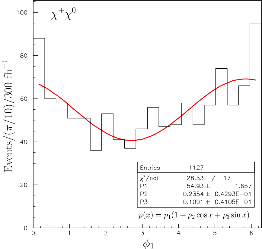

Non-trivial azimuthal-angle distributions show up when there is parity and/or CP violation in the decay vertex. In order to measure this, we need to completely reconstruct the kinematics such as the angle . The angle is expressed in terms of the angle and the three-momentum of in the CM frame:
| (118) |
with
In order to define the CM frame in Fig. 1, we need to know the direction of the anti-quark which can be determined only statistically in -collision experiments. We take the -direction to be the same direction as that of the total momentum, , in the laboratory frame since the parton tends to carry a smaller momentum. In order to reduce the number of mis-choices, we impose a cut: GeV.
The dependent part of the distribution in Eq. (91) has opposite signs for and productions. We do not impose a cut on because the function in Eq. (92) takes its maximum value at the threshold production. (In order to look for a CP asymmetry, it may be better to impose a cut. See Eq. (93).) We also use both solutions for . The averaged value of the functions and are:
| (122) |
We expect that these values will be affected due to the existence of the false solution.
The distributions are shown in Fig. 13 with 300 fb-1 of data. The left figure is the distribution of the events (i.e., the events with a positive-charge lepton) and the right figure is from the events. We fit the histogram by a function:
| (123) |
A qualitatively correct behavior is obtained in the events, i.e., and , but events do not show the expected behavior of and due to poor statistics and the selection cut on . We can see from the figures that the selection cut on tends to give a fake distribution peaked near and for both and events. One may be able to avoid this by imposing the cut on both solutions as we have done in the study of the distribution, but it significantly reduces the statistics. A looser cut on results in a fake distribution by the mis-choice of the -direction. Nevertheless, it is not a problem for observing a non-trivial distribution since the theoretic distribution is different for and productions. For example, one can try to rescale the histogram of the events and subtract from (or add to) that of the events in order to eliminate (or understand) the fake distribution.
6.3.6 distribution
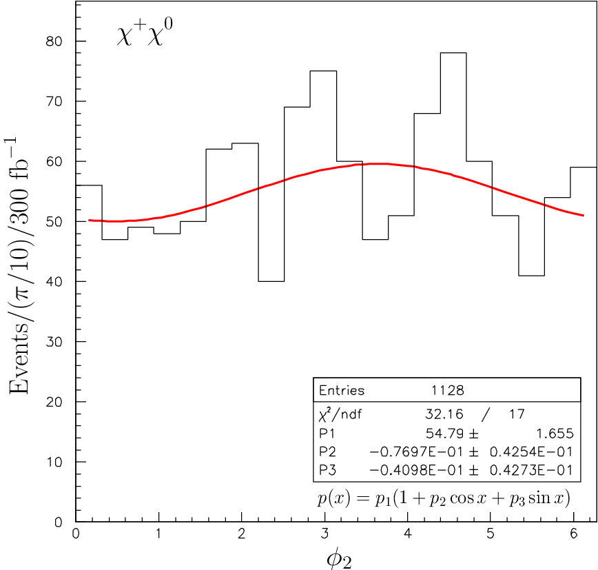

The distribution can be obtained by the same method. The distribution clearly shows an expected behavior in Eq. (94) with and .
7 Summary
If is the lightest among the superpartners of the Standard Model particles, the SUSY signatures at the LHC experiments will be very different from the stable neutralino scenario. We have demonstrated that the production processes of the neutralinos and charginos have rich information on model parameters. The spin correlations of intermediate particles give rise to interesting non-trivial distributions in various kinematic variables. In previous studies of SUSY models at hadron colliders, the production of neutralinos and charginos have been usually thought of as good processes to discover SUSY through multi-lepton final states. In the stable neutralino scenario it is nevertheless challenging to extract information on models out of those processes because of the small cross sections and difficult kinematics due to escaping neutralinos. Much attention has been paid to production processes of colored superparticles and their cascade decays for the measurements of the model parameters. However, as we have shown, the chargino-neutralino production process may provide us with the best opportunity for understanding SUSY models in the long-lived scenario.
The study presented in this paper is not fully realistic in several senses. We have not included the momentum resolution of the tracks or efficiency of the identification. Also, in the study of various distributions, we have ignored errors in the measurements of the chargino and the neutralino masses. We have used the transverse missing momentum evaluated by the fast detector simulator, but the resolution may be very different in real experiments. The trigger efficiency of the process has also been ignored. A more detailed analysis is necessary when we discover the long-lived . The analytical formulae presented in this paper will be useful in such future studies.
This work is inspired by studies of the electroweak theory in Refs. [33] where the differential cross section of the process is calculated including the effect of spin correlations. These various distributions are studied for the purpose of confirming the SU(2)L U(1)Y gauge interactions. The density matrix calculated there has been used to put constraints on anomalous interactions among gauge bosons at the LEP-II experiments [34]. If is long-lived, the cross-section formula calculated in this paper can be used as a good test of SUSY at the LHC experiments just like we have confirmed the Standard Model at the LEP experiments.
We here comment on the production processes which we did not study in this paper. In many cases, these processes have smaller cross sections than the process. Since the -boson vertex involving the same mass eigenstates, , vanishes identically, the main production process is with . If we require the opposite charges for two ’s and the leptonic decays for both of the leptons, the number of events will get smaller. However, for the reconstruction of the kinematics, it is much simpler than the production events. We can reconstruct the final state without the knowledge of the neutralino masses. Moreover, there is no discrete ambiguity for the reconstruction. The study of these processes will also be important if is long-lived, although it may be challenging due to the limited statistics.
Acknowledgments
I thank Michael Graesser for reading the manuscript, stimulating discussions and useful comments. I also thank Alex Friedland for discussions and useful comments.
References
- [1] T. Gherghetta, G. F. Giudice and A. Riotto, Phys. Lett. B 446, 28 (1999) [arXiv:hep-ph/9808401]; T. Asaka, K. Hamaguchi and K. Suzuki, Phys. Lett. B 490, 136 (2000) [arXiv:hep-ph/0005136]; J. L. Feng, S. Su and F. Takayama, Phys. Rev. D 70, 075019 (2004) [arXiv:hep-ph/0404231]; M. Pospelov, Phys. Rev. Lett. 98, 231301 (2007) [arXiv:hep-ph/0605215]; K. Kohri and F. Takayama, Phys. Rev. D 76, 063507 (2007) [arXiv:hep-ph/0605243]; M. Kawasaki, K. Kohri and T. Moroi, Phys. Lett. B 649, 436 (2007) [arXiv:hep-ph/0703122]; J. Pradler and F. D. Steffen, arXiv:0710.2213 [hep-ph]; K. Jedamzik, JCAP 0803, 008 (2008) [arXiv:0710.5153 [hep-ph]]; M. Kawasaki, K. Kohri, T. Moroi and A. Yotsuyanagi, arXiv:0804.3745 [hep-ph].
- [2] T. Moroi, H. Murayama and M. Yamaguchi, Phys. Lett. B 303, 289 (1993); E. Holtmann, M. Kawasaki, K. Kohri and T. Moroi, Phys. Rev. D 60, 023506 (1999) [arXiv:hep-ph/9805405]; J. L. Feng, A. Rajaraman and F. Takayama, Phys. Rev. Lett. 91, 011302 (2003) [arXiv:hep-ph/0302215]; J. L. Feng, A. Rajaraman and F. Takayama, Phys. Rev. D 68, 063504 (2003) [arXiv:hep-ph/0306024]; J. L. Feng, S. f. Su and F. Takayama, Phys. Rev. D 70, 063514 (2004) [arXiv:hep-ph/0404198]; M. Kawasaki, K. Kohri and T. Moroi, Phys. Lett. B 625, 7 (2005) [arXiv:astro-ph/0402490]; M. Kawasaki, K. Kohri and T. Moroi, Phys. Rev. D 71, 083502 (2005) [arXiv:astro-ph/0408426].
- [3] M. Ibe and R. Kitano, JHEP 0708, 016 (2007) [arXiv:0705.3686 [hep-ph]].
- [4] I. Hinchliffe and F. E. Paige, Phys. Rev. D 60, 095002 (1999) [arXiv:hep-ph/9812233].
- [5] J. R. Ellis, A. R. Raklev and O. K. Oye, JHEP 0610, 061 (2006) [arXiv:hep-ph/0607261].
- [6] A. Nisati, S. Petrarca and G. Salvini, Mod. Phys. Lett. A 12, 2213 (1997) [arXiv:hep-ph/9707376].
- [7] G. Polesello and A. Rimoldi, ATLAS Internal Note ATL-MUON-99-006.
- [8] S. Ambrosanio, B. Mele, S. Petrarca, G. Polesello and A. Rimoldi, JHEP 0101, 014 (2001) [arXiv:hep-ph/0010081].
- [9] J. Ellis, A. R. Raklev and O. K. Oye, ATLAS Note ATL-PHYS-PUB-2007-016; ATL-COM-PHYS-2006-093.
- [10] W. Buchmuller, K. Hamaguchi, M. Ratz and T. Yanagida, Phys. Lett. B 588, 90 (2004) [arXiv:hep-ph/0402179].
- [11] K. Hamaguchi, Y. Kuno, T. Nakaya and M. M. Nojiri, Phys. Rev. D 70, 115007 (2004) [arXiv:hep-ph/0409248].
- [12] J. L. Feng and B. T. Smith, Phys. Rev. D 71, 015004 (2005) [Erratum-ibid. D 71, 019904 (2005)] [arXiv:hep-ph/0409278].
- [13] A. Rajaraman and B. T. Smith, Phys. Rev. D 76, 115004 (2007) [arXiv:0708.3100 [hep-ph]].
- [14] M. Drees and X. Tata, Phys. Lett. B 252, 695 (1990).
- [15] J. L. Feng and T. Moroi, Phys. Rev. D 58, 035001 (1998) [arXiv:hep-ph/9712499].
- [16] S. P. Martin and J. D. Wells, Phys. Rev. D 59, 035008 (1999) [arXiv:hep-ph/9805289].
- [17] S. Dimopoulos, S. D. Thomas and J. D. Wells, Nucl. Phys. B 488, 39 (1997) [arXiv:hep-ph/9609434].
- [18] S. K. Gupta, B. Mukhopadhyaya and S. K. Rai, Phys. Rev. D 75, 075007 (2007) [arXiv:hep-ph/0701063].
- [19] V. D. Barger, R. W. Robinett, W. Y. Keung and R. J. N. Phillips, Phys. Lett. B 131, 372 (1983).
- [20] H. E. Haber, arXiv:hep-ph/9405376.
- [21] B. K. Bullock, K. Hagiwara and A. D. Martin, Nucl. Phys. B 395, 499 (1993).
- [22] M. R. Buckley, H. Murayama, W. Klemm and V. Rentala, arXiv:0711.0364 [hep-ph].
- [23] G. Corcella et al., arXiv:hep-ph/0210213.
- [24] P. Richardson, JHEP 0111, 029 (2001) [arXiv:hep-ph/0110108].
- [25] S. Moretti, K. Odagiri, P. Richardson, M. H. Seymour and B. R. Webber, JHEP 0204, 028 (2002) [arXiv:hep-ph/0204123].
- [26] H. L. Lai et al. [CTEQ Collaboration], Eur. Phys. J. C 12, 375 (2000) [arXiv:hep-ph/9903282].
- [27] S. Jadach, Z. Was, R. Decker and J. H. Kuhn, Comput. Phys. Commun. 76, 361 (1993).
- [28] E. Richter-Was, arXiv:hep-ph/0207355.
- [29] C. G. Lester and D. J. Summers, Phys. Lett. B 463, 99 (1999) [arXiv:hep-ph/9906349].
- [30] K. Kawagoe, M. M. Nojiri and G. Polesello, Phys. Rev. D 71, 035008 (2005) [arXiv:hep-ph/0410160].
- [31] H. C. Cheng, J. F. Gunion, Z. Han, G. Marandella and B. McElrath, JHEP 0712, 076 (2007) [arXiv:0707.0030 [hep-ph]].
- [32] M. Davids et al., CMS Note 2006/077.
- [33] K. J. F. Gaemers and G. J. Gounaris, Z. Phys. C 1, 259 (1979); K. Hagiwara, R. D. Peccei, D. Zeppenfeld and K. Hikasa, Nucl. Phys. B 282, 253 (1987); P. Mery, M. Perrottet and F. M. Renard, Z. Phys. C 36, 249 (1987); M. S. Bilenky, J. L. Kneur, F. M. Renard and D. Schildknecht, Nucl. Phys. B 409, 22 (1993).
- [34] P. Abreu et al. [DELPHI Collaboration], Phys. Lett. B 502 (2001) 9 [arXiv:hep-ex/0102041]; P. Achard et al. [L3 Collaboration], Phys. Lett. B 586, 151 (2004) [arXiv:hep-ex/0402036]; S. Schael et al. [ALEPH Collaboration], Phys. Lett. B 614 (2005) 7; J. Abdallah et al. [DELPHI Collaboration], Eur. Phys. J. C 54, 345 (2008) [arXiv:0801.1235 [hep-ex]].